Optimizing Critical Overloaded Power Transmission Lines with a Novel Unified SVC Deployment Approach Based on FVSI Analysis

Abstract

This paper proposes a novel methodology to improve stability in a transmission system under critical conditions of operation when additional loads that take the system to the verge of stability are placed in weak bus bars according to the fast voltage stability index (FVSI). This paper employs the Newton–Raphson method to calculate power flows accurately and, based on that information, correctly calculate the FVSI for every transmission line. First, the weakest transmission line is identified by considering $N-1$ contingencies for the disconnection of transmission lines, and then all weak nodes associated with this transmission line are identified. Following this, critical scenarios generated by stochastically placed loads that will take the system to the verge of instability will be placed on the identified weak nodes. Then, the methodology will optimally size and place a single static VAR compensator SVC in the system to take the transmission system to the conditions before the additional loads are connected. Finally, the methodology will be validated by testing the system for critical contingencies when any transmission line associated with the weak nodes is disconnected. As a result, this paper’s methodology found a single SVC that will improve the system’s stability and voltage profiles to similar values when the additional loads are not connected and even before contingencies occur. The methodology is validated on three transmission systems: IEEE 14, 30, and 118 bus bars.

1. Introduction

1.1. Literature Review

The authors in [1] presented a work that aimed to determine the optimal placement of FACTS devices based on contingency ranking, targeting the enhancement of the voltage stability margin (VSM) under various system loading conditions. The research deployed FACTS devices at strategic locations identified through an analytical framework to enhance voltage stability.

The research in [2] aimed to enhance the resiliency and transient response of power electronic-dominated grids through an AI-based power reference correction (AI-PRC) module for grid-following inverter GFLIs, allowing them to adjust their power setpoints autonomously during transient disturbances. The paper identified critical buses and lines using various indices to determine the optimal placement of FACTS devices that enhance voltage stability.

In [3], the authors aimed to enhance the power system’s stability and reliability by addressing two challenges: reactive power planning (RPP) and voltage stability improvement (VSI). For this purpose, a multi-objective genetic algorithm (MOGA) for RPP was used, focusing on minimizing power loss costs, maximizing the use of new reactive power (VAR) sources, enhancing VSI, and improving total transfer capacity (TTC).

The objective in [4] was to enhance power system transient stability using modern power system stabilizers (PSSs) combined with FACTS controllers by implementing an SSSC-based controller. The article proposed a methodology for selecting the most efficient wide-area signals and controller locations based on a geometric measure of a joint controllability/observability index. The study confirmed that FACTS controllers, particularly the SSSC, effectively improved power system stability and the handling of transient disturbances. This significant result highlights the importance of advanced control strategies in power systems.

The researchers in [5] presented a comparative analysis of solutions for improving transient stability in electrical power systems (EPSs). The solutions included rotor angle and frequency stability analysis. The solutions presented by the researchers included a static VAR compensator (SVC), a static synchronous compensator (STATCOM), a fast excitation system, and an additional parallel transmission line. As a study case, the IEEE 9-bus bar system was selected.

In [6], the paper’s main objective was to improve voltage stability and maintain synchronism in power systems that include wind farms. The impact of wind speed variability on power generation reliability was mitigated by an optimized battery energy storage system (BESS) and a unique solution presented by the authors that self-corrects the static volt-ampere reactive compensator (SVC). The solution was tested by comparing network voltage profiles before and after voltage deviations.

The authors in [7] proposed to improve power system stability and control by optimally placing FACTS devices within a power grid. The researchers developed a new algorithm called the filter feeding allogenic engineering (FFAE) algorithm for their study. The research paper focuses on Kenya’s 87-bus 25-generator 132 kV and 220 kV transmission network. The researchers conducted simulations within MATLAB’s environment to achieve two objectives: minimizing the active power loss and voltage deviations.

In [8], the authors proposed the enhancement of power system stability through the optimal allocation of unified power flow controllers (UPFCs). The research proposed a modified particle swarm optimization (PSO) algorithm to determine the most effective locations and settings for UPFC devices within the IEEE 30-bus test system. The study was evaluated based on reducing active and reactive power losses, improving voltage profiles, and enhancing the system’s transient stability during sudden disturbances.

The authors in [9] developed energy functions (EFs) for static synchronous compensators (STATCOMs), considering their control strategies and limitations, to facilitate energy-function-based transient stability assessment and improvement methods. The work proved that the EF-based control strategies optimize the transient stability of EPSs globally, serving as a benchmark for simpler, more applicable control strategies. It illustrated how STATCOM and RES can be dynamically managed to significantly improve transient stability.

In [10], the authors aimed to assess the effectiveness of various methods and tools in improving the efficiency and reliability of power distribution systems. These methods included implementing FACTS devices, optimizing algorithms to determine the best placement and sizing of these devices, and developing innovative control strategies for existing network components. To achieve this goal, the authors utilized genetic algorithms, particle swarm optimization, and other metaheuristic approaches to find these technologies’ optimal configuration, sizing, and placement.

In [11], researchers aimed to enhance the stability and security of a microgrid with wind energy through conversion systems (WECSs), specifically double-fed induction generators (DFIGs). For this purpose, the optimal placement of a unified power flow controller (UPFC) was employed with the help of the non-dominated sorting genetic algorithm II (NSGA-II). The optimization problem considered two variables: maximizing stability and minimizing active power losses. Finally, the authors demonstrated the capability of the UPFC to control line flow and voltage, thus increasing the system’s load capacity.

The research presented by [12] aimed to improve the transient stability of EPSs that employed UPFCs. This improvement was achieved by developing a nonlinear control technique using the direct Lyapunov method. The authors developed a damping control for the power system with UPFC using the transient energy function (TEF) method and additional control via a second-order sliding mode observer (SMO). The results indicated an improvement in the transient stability of the system by reducing the first swing of oscillations and increasing stability margins.

In [13], the paper suggested a different approach to the traditional use of STATCOM and presented a secondary function for it: oscillation damping, improved transient stability, and enhanced power network security. A network model with a synchronous generator, transformer, loads, and a shunt-connected STATCOM was considered to enhance oscillation damping and improve transient stability and network security during large disturbances.

In [14], the authors optimized the placement and sizing of STATCOMs within the power system to enhance bus voltage stability and minimize power losses, addressing challenges posed by an increased power demand and limitations on new transmission capacity. The research used the whale optimization algorithm (WOA), which formulates an objective function that includes factors such as voltage deviation, STATCOM size, and active and reactive power losses.

The research in [15] employed a back–forward load flow technique for power flow modeling, with the improved bacterial foraging algorithm used for determining the optimal location and size of DSTATCOM. The study showed that IBFA outperformed traditional optimization methods, reducing power loss and improving DSTATCOM placement and sizing voltage stability.

In [16], the authors focused on suppressing low-frequency oscillation (LFO) in wind–PV–thermal-bundled power transmission systems by coordinating the design of multiple FACTS devices, including a static synchronous compensator (STATCOM) and a static synchronous series compensator (SSSC). A PSO-GA algorithm successfully optimizes the parameters of the PSS, SSSC-PODC, and STATCOM-PODC, demonstrating a notable improvement in system stability compared to scenarios where FACTS devices are not optimally coordinated.

The authors in [17] presented a new methodology for contingency ranking in radial distribution systems, which mainly considers voltage stability indexes. The methodology identified system vulnerabilities and then improved the reliability by assessing the impact of contingencies such as the loss of FACTS devices, distributed generation (DG) sets, and lines on voltage stability.

The authors in [18] proposed a hybrid firefly and particle swarm optimization algorithm (HFPSO) for the optimal placement and sizing of DG and D-STATCOM in a radial distribution system (RDS). This research aimed to improve voltage stability, enhance the voltage profile, and minimize power loss. The paper demonstrates a significant reduction in power loss and improved voltage stability across the distribution network.

In [19], researchers aimed to enhance power system stability through voltage control, reactive power, and power factor improvement using a static synchronous compensator (STATCOM) equipped with serial multicellular converters. The paper proposed a control model based on the shifted pulse width modulation (PS-PWM) technique. This was selected for its simplicity, low total harmonic distortion (THD), and suitability for cascaded inverters.

As a summary,

Table 1. Consolidated summary of research papers.

Author	Methodologies	Test System	Voltage Profile	Power Losses	Stability Indexes	Cost	Variable Loads
[1,10]	Analytical Modeling, Simulation, Optimization Techniques	IEEE 14-bus system, NRPG 246-bus system	✓	✓	-	-	✓
[2,9,13,16]	Control Strategy Development, Simulation, and Testing	SMIB and IEEE 9-bus systems, 14-bus systems	-	-	✓	-	✓
[3,8,18]	Optimization Algorithms for FACTS Devices	Modified IEEE 30-bus system, South Egypt Electricity network, IEEE 33-bus and Iraqi 65-bus systems	✓	✓	✓	-	✓
[4,5]	Simulation, SCR Variation Analysis	IEEE 9-bus system	-	-	✓	✓	-
[6,13]	FACTS Devices Integration in Renewable Energy Systems	Wind farms with PMSG, Multi-machine network model	✓	-	✓	-	✓
[7,14,15]	Algorithm-Based FACTS Devices Optimization	Kenya’s 87-bus 25-generator Network, Quha feeder, Lachi distribution network	✓	✓	-	-	✓
[11,17]	NSGA-II Optimization, Contingency Ranking	Modified IEEE 14-bus system	-	✓	✓	-	✓
[19]	Serial Multicellular Converters Integration	MATLAB Simulink model	✓	-	✓	-	✓

shows the methodologies employed in stability analysis and improvement in transmission systems. Among those methodologies, various optimization techniques have been selected, showing that no new models or techniques have been developed in recent years. Also, according to this analysis, only variable loads have been considered, and the impact of critical loads in weak nodes in the system has not been adequately studied. Therefore, this paper aims to provide a new methodology by proposing a novel algorithm that considers the impact of the stochastic placement of loads in weak power nodes.

1.2. Organization

Section 1: This presents the paper’s introduction and review of the state of the art in different techniques employed for stability improvement in transmission systems.

Section 2: This section explains the methods for optimal SVC placement and sizing for a system that works under critical conditions with considerable loads in weak nodes in a transmission system.

Section 3: This section presents the application of this paper’s methodology in three study cases, IEEE 14, 30, and 118 transmission systems, and the metrics and statistical analysis.

Section 4: Conclusions: this presents an overview of the quantitative results obtained in the different study cases; the conclusions validate the methodology that this paper proposes.

Section 5: Future work and challenges: this outlines future challenges for complex analysts to consider to further improve stability in a transmission system under unpredictable conditions such as time variable loads and stability indexes.

2. Methodology

This paper proposes a methodology in which the nodes associated with the weakest transmission line (close to instability) in an electrical transmission system will be identified based on the stability criterion of the fast voltage stability index (FVSI). Then, under connection scenarios of stochastic loads and overload of these weak nodes, a methodology is proposed in which, through a single static VAR compensator SVC, the stability levels of all lines can be reestablished to values before the overload of the system. In addition, the methodology will consider an improvement in the voltage profiles. Subsequently, to validate the method, $N-1$ contingencies will be carried out on the lines associated with the weak nodes previously identified and thus verify that even in disconnection scenarios, the system will operate in conditions as close as possible to the scenario before disconnection and before overloading the system with stochastic loads.

The methodology proposed in this paper is explained in detail in the following sections, starting with concepts essential for the method proposed in this research.

2.1. Power Flow Calculations: Newton–Raphson

Various mathematical methods are used to calculate electrical variables in an electrical power system. Among these methods, the Newton–Raphson (NR) method is one of the most commonly used and provides greater precision in computed values. The NR method involves the solution of nonlinear equations that are obtained from Kirchhoff’s laws. The nonlinear equations are formulated based on active power ($P_i$) and reactive power ($Q_i$), which, in turn, are functions of voltage magnitude $V_i$ and angle (${\delta }_i$). Active and reactive power expressions are shown in Equations (1) and (2), respectively [20].

$$P_i\left(x\right)=\sum _{j=1}^n\left|V_i\right|\left|V_j\right|\left(G_{i-j}cos{\delta }_{i-j}+B_{i-j}sin{\delta }_{i-j}\right)$$

(1)

$$Q_i\left(x\right)=\sum _{j=1}^n\left|V_i\right|\left|V_j\right|\left(G_{i-j}sin{\delta }_{i-j}-B_{i-j}cos{\delta }_{i-j}\right)$$

(2)

For Equations (1) and (2), the sub-index i represents the sending node or bus bar and the subindex j is the receiving node. Also, $G_{i-j}$ is the conductance and $B_{i-j}$ is the substance for a power line $i-j$.

A solution obtained by the Newton–Raphson method describes the behavior of the flow of active and reactive power in an EPS. Results are obtained through iterative calculations that update the estimated values of voltages and angles. Iterations are represented by the letter k, and Equation (3) describes the entire process [20].

$$x^{(k+1)}=x^{\left(k\right)}-{\left[J\left(x^{\left(k\right)}\right)\right]}^{-1}f\left(x^{\left(k\right)}\right)$$

(3)

In Equation (3), $(k+1)$ represents the current iteration, $\left(k\right)$ is the previous one, and J is the Jacobian matrix. This matrix contains partial derivatives of the power flow equations with respect to the voltage angles and magnitudes, as can be seen in Equation (4).

$$J\left(x\right)=\left[\begin{array}{cccc}\frac{\partial f1}{\partial x_1}\left(x\right)& \frac{\partial f1}{\partial x_2}\left(x\right)& \dots & \frac{\partial f1}{\partial x_{2n-2}}\left(x\right)\\ \frac{\partial f2}{\partial x_1}\left(x\right)& \frac{\partial f2}{\partial x_2}\left(x\right)& \dots & \frac{\partial f2}{\partial x_{2n-2}}\left(x\right)\\ .& .& .& .\\ .& .& .& .\\ \frac{\partial f_{2n-2}}{\partial x_1}\left(x\right)& \frac{\partial f_{2n-2}}{\partial x_2}\left(x\right)& \dots & \frac{\partial f_{2n-2}}{\partial x_{2n-2}}\left(x\right)\end{array}\right]$$

(4)

2.2. Stability for Transmission Lines: Fast Voltage Stability Index (FVSI)

The fast voltage stability index (FVSI) is one of the most commonly used stability indices in analyzing an electrical power system’s reliability. It is a non-dimensional value that evaluates the voltage stability in transmission lines of a system under different load ability conditions. This index quickly and efficiently provides a parameter to assess how close the transmission lines are to the point of instability. The closer the index is to one, the closer the line is to instability. This is crucial for the planning, operation, and reliability of electrical power systems [21].

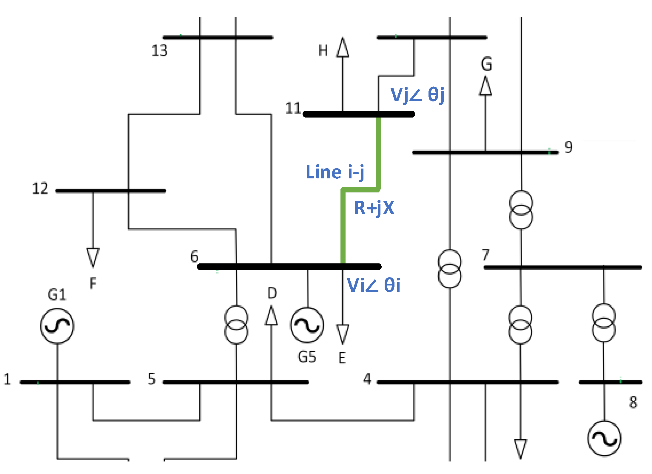
Figure 1 shows a section of the IEEE 14-bus bar transmission system in which the FVSI is analyzed in power line _6–11. In this graph, $V_i\angle {\delta }_i$ is the voltage magnitude and angle at the sending bus bar i (in this example, bus bar 6), also $V_j\angle {\delta }_j$ is the voltage magnitude and angle at the receiving bus bar j (in this example, bus bar 11). Finally, line $i-j$ ($6–11$) has an impedance of $Z_{i-j}=R_{i-j}+j{X}_{i-j}$.

After showing the components involved with FVSI calculations, the calculation itself is described in Equation (5), where the sub-index i is associated with the sending bus bar, j represents the receiving bus bar, $Q_j$ is the receiving reactive power at node j from node i, $V_i$ is the voltage magnitude at the sending bus bar, $X_{i-j}$ is the reactance of line $i-j$, and $Z_{i-j}$ is the impedance of line $i-j$.

$$FVS{I}_{i-j}=\frac{4Z_{i-j}{Q}_j}{V_i^2{X}_{i-j}}$$

(5)

According to research in [20], the apparent power received at node j from node i can be described as shown in Equation (6), and by considering that $V_i=\left|V_i\right|e^{j{\delta }_i}$, $V_j=\left|V_j\right|e^{j{\delta }_j}$ and $Z_{ij}=R_{i-j}+j{X}_{i-j}$, the reactive power that is received at node j from node i ($Q_j$) can be calculated as described in Equation (7). Therefore, after power flows are solved by Newton–Raphson equations, the FVSI for every transmission line can be calculated by integrating Equation (7) into Equation (5).

$$S_{j-i}=V_j{\left(\frac{V_j-V_i}{Z_{i-j}}\right)}^{\ast }$$

(6)

$$Q_j=-V_j^2{B}_{i-j}-V_i{V}_j\left[G_{i-j}sin\left({\delta }_{j-i}\right)-B_{i-j}cos\left({\delta }_{j-i}\right)\right]$$

(7)

2.3. Description of the Proposed Methodology

2.3.1. Stage 1: Identification of Weakest Transmission Line

The following process is required to calculate FVSIs for a transmission system. Firstly, all the electrical parameters of buses, lines, generators, and system loads are initialized and loaded. After that, a power flow is run using the Newton–Raphson method to obtain each node’s voltage and angle parameters. With these parameters, the FVSI values are then calculated and stored in a variable corresponding to the line they represent. All of these values are stored in the variable for future reference. This process is fully detailed in Algorithm 1.

Algorithm 1: FVSI calculation for all power lines in a system

Step: 1  Load System Data      Base electrical parameters from lines, buses, generators, and loads      $SystemData\leftarrow LoadSystemData(Bu{s}_{data},Ge{n}_{data},Lin{e}_{data},Loa{d}_{data})$ Step: 2  Power Flow Calulations      By executing Newton–Raphson method:      $V_i$, $V_j$, ${\delta }_i$, ${\delta }_j$$\leftarrow PowerFlowAnalysis\left(SystemData\right)$ Step: 3  Reactive power $Q_j$ and FVSI calculation for each line      for$k=1:Numberoflines$      ${\delta }_{j-i}\left(k\right)={\delta }_j\left(k\right)-{\delta }_i\left(k\right)$      $Q_j\left(k\right)=-V_i{\left(k\right)}^2{B}_{i-j}\left(k\right)-V_i\left(k\right)V_j\left(k\right)\left[G_{i-j}\left(k\right)sin\left({\delta }_{j-i}\left(k\right)\right)-B_{i-j}cos\left({\delta }_{j-i}\left(k\right)\right)\right]$      $FVSI=\frac{4Z_{i-j}\left(k\right)Q_j\left(k\right)}{V_i{\left(k\right)}^2{X}_{i-j}}$      $FVS{I}_{global}(:,k)=[FVSI,lin{e}_{i-j}]$      end for Step: 4  Return results      $FVS{I}_{global}$

Subsequently, it is necessary to identify the weakest transmission line in the system based on the FVSI calculation and consider all line disconnection scenarios, including criterion $N-1$. For this, the FVSI of the entire system will be calculated in each scenario in which a line is disconnected. Later, when all the scenarios have been calculated, the line with the greatest coincidences with the highest FVSI will be determined, determining the weakest line of the entire system in all $N-1$ scenarios. This process is fully explained in Algorithm 2.

Algorithm 2: Identify the weakest power line by FVSI analysis in $N-1$ scenarios

Step: 1  Initialization      $Lin{e}_{data}\leftarrow LoadLines\left(\right)$      $N\leftarrow |Lin{e}_{data}|$      $FVS{I}_{scenarios}\leftarrow \left[\right]$ Step: 2  For each line removal scenario, calculate FVSI      for  $i=1$  to  N  do      $Lin{e}_{data}^{\left(i\right)}\leftarrow RemoveLine(Lin{e}_{data},i)$      $FVS{I}_{global}^{\left(i\right)}\leftarrow CalculateFVSI\left(Lin{e}_{data}^{\left(i\right)}\right)$      $FVS{I}_{scenarios}\left[i\right]\leftarrow FVS{I}_{global}^{\left(i\right)}$      end for Step: 3  Identify the weakest line      $Weakes{t}_{line}\leftarrow FindWeakestLine\left(FVS{I}_{scenarios}\right)$ Step: 4  Output the result      return  $Weakes{t}_{line}$

2.3.2. Stage 2: Critical Overloading of Bus Bars Associated with the Weakest Transmission Line

The next stage of this work is analyzing the most critical system overload scenarios. Once the weakest line $i-j$ has been identified, all lines connected with the sending node i or the receiving node j will be identified. This is performed to identify all nodes that have some direct connection with the weakest line. Subsequently, the maximum load value to be included in the system will be defined before it becomes unstable. This load value will be distributed randomly among 50% of the identified weak nodes. From this, M scenarios will be created with random loads, in which the distribution of each load will be 80% for the active part and 20% for the reactive part. Finally, all these scenarios will be the analysis point for the solution proposed in this paper. This is fully detailed in Algorithm 3.

Algorithm 3: Critical load placement for nodes associated with the weakest line

Step: 1  Identify Weakest Line ($WL$)      $WL\leftarrow FindWeakestLine\left(\right)\leftarrow From:Algorith{m}_2$ Step: 2  Select Nodes ($CN$)      $CN\leftarrow GetConnectedNodes\left(WL\right)\setminus \{PV,Slack\}$ Step: 3  Stochastic Load Allocation      for  $s=1$  to  M  do      $S{N}_s\leftarrow RandomSubset(CN,50\%)$      $LoadAllo{c}_s\leftarrow DistributeLoads(S{N}_s,MAXP,MAXQ)$      end for Step: 4  Output Load Scenarios      return  $LoadAllo{c}_1,\dots ,LoadAllo{c}_M$

2.3.3. Stage 3: Optimal SVC Sizing and Placement for Scenarios of Critical Overloading in Weakest Buses

Once critical load scenarios have been created and placed randomly on the weak buses associated with the weakest line, the next step is to identify the node in which placing the SVC will cause the FVSI values to be corrected or brought as close as possible to the values before these critical states of the system. For this, SVCs with values from 5MVAR to a maximum value that has been defined as 100MVAR will be placed in each bus bar, and all possible combinations will be compared with the original FVSI values to obtain the best solution without having to depend on the maximum SVC possible, which will reduce costs; this process is fully explained in Algorithm 4.

This algorithm has been designed so that this optimal solution improves the system’s operating conditions before the critical loadability conditions and guarantees that the system maintains these conditions in the event of the disconnection of $N-1$ lines.

Algorithm 4: Optimal SVC location and sizing based on critical loading scenarios

Step: 1  Load M Load Allocation Scenarios from Algorithm 3      $LoadScenarios\leftarrow LoadFromAlgorithm3\left(\right)$ Step: 2  Calculate Original FVSI for Each Scenario      for each  $scenario$  in  $LoadScenarios$  do      $FVS{I}_{original}\leftarrow CalculateFVSI\left(scenario\right)$      end for Step: 3  Apply SVC Optimization Directly for Each Scenario      for each  $scenario$  in  $LoadScenarios$  do      $OptimalSVC\leftarrow \left[\right]$      for  $k=1$  to  $Numberofbuses$  do       if  $bu{s}_k$  is not  $P{V}_{bus}$  and  $bu{s}_k$  is not  $Slac{k}_{bus}$  then        for $m=5$ step 5 to $maxComp$ do         $Q_{SVC}^{(k,m)}\leftarrow m$         $FVS{I}_{scenario}^{(k,m)}\leftarrow CalculateFVSIWithSVC(scenario,k,Q_{SVC}^{(k,m)})$         if  $|FVS{I}_{scenario}^{(k,m)}-FVS{I}_{original}|$  is minimized then           $OptimalSVC\leftarrow [k,m,FVS{I}_{scenario}^{(k,m)}]$        end for       end if      end for      $Result{s}_{scenario}\leftarrow OptimalSVC$      end for Step: 4  Return Optimal SVC Locations and Sizes for Each Scenario      return  $Results$

2.3.4. Stage 4: Results Validation for $N-1$ Scenarios

In stage 3, this research found the optimal location and sizing of an SVC for any random critical load allocation scenarios to establish the FVSIs to values before loads were connected. However, this methodology will guarantee this success under overloading and when $N-1$ contingencies for line disconnections are applied to this overloading scenario. Therefore, this final stage will generate all possible contingency scenarios and evaluate FVSIs.

2.4. Case Studies

The proposed methodology will be tested and validated in three transmission systems: IEEE 14, 30, and 118 bus bars. These case studies were chosen to verify the methodology’s effectiveness in various scenarios and to assess its scalability as the system’s complexity increases with its size. This testing will ensure the methodology’s validation across all transmission systems.

The electrical power systems in the United States inspired the selection of the chosen transmission systems. These systems were picked due to their configurations, structures, and characteristics, making them the most suitable for electrical and energy research.

3. Analysis of Results

3.1. Case Study: IEEE 14-Bus Bar System

3.1.1. Weakest Power Line by Analyzing $N-1$ Contingency Scenarios

The IEEE 14-bar system consists of a total of 20 transmission lines. Therefore, in this analysis, each possible contingency was executed when disconnecting each line; 20 line disconnection scenarios were analyzed. Each analysis returned FVSI values for each line, as seen in the example in

Table 2. Example of FVSI at IEEE 14 when $lin{e}_{2–4}$ is disconnected.

Transmission Line		FVSI	Transmission Line		FVSI
Sending Node $\mathit{i}$	Receiving Node $\mathit{j}$		Sending Node $\mathit{i}$	Receiving Node $\mathit{j}$
2	5	0.1392	9	10	0.0211
10	11	0.1154	6	12	0.0182
1	5	0.1108	4	5	0.0181
13	14	0.0919	3	4	0.0150
2	3	0.0889	6	13	0.0136
4	9	0.0682	6	11	0.0130
7	8	0.0621	1	2	0.0062
7	9	0.0479	12	13	0.0052
4	7	0.0261	9	14	0.0030
5	6	0.0248

, in which power $lin{e}_{2–4}$ was disconnected.

After applying Algorithm 2 and analyzing all possible contingencies, it was found that the most repeated lines under this analysis (higher FVSIs) were the weakest when it came to cases of instability based on the FVSI.

Table 3. FVSI average value, count, and percentage for selected nodes for all $N-1$ contingencies.

Power Line		FVSI AvgValue	Count	Percentage [%]
Node $\mathit{i}$	Node $\mathit{j}$
2	5	0.1392	15	75
3	4	0.1752	1	5
10	11	0.1448	4	20

shows the percentage results and the average FVSI value obtained from the line when it was detected as the weakest.

Based on these results, it can be determined that in 75% of the contingency scenarios, $lin{e}_{2-5}$ is the weakest, and based on this, it will be taken as a starting point that sending node 2 and receiving node 5 will be the weakest nodes for the subsequent analysis of this work.

3.1.2. Overloading of Critical Nodes

When applying Algorithm 3 based on the results of Algorithm 2, all the associated nodes nearby through a single power line connection with the weakest nodes (2 and 5) were found. The power nodes identified were nodes 2, 3, 4, 5, and 6. Node 1 was also nearby; however, the algorithm discards PV buses and the slack bus.

Before connecting the additional loads in the system, it is imperative to determine the maximum additional load possible to connect to the system before instability. Based on the criteria detailed in [22], the highest load connected in the IEEE 14-bus bar system is 94 MW and node 3, and therefore, by performing multiple power flow analyses, it was found that this maximum load can be increased up to 220%. Therefore, this research will take a maximum load into that maximum range. Thus, 150 MW will be taken as the additional load to be connected to the system.

The maximum load of 150 MW will be stochastically distributed between at least 50% of the previously detected weakest nodes. Each load will also comprise 80% active power and 20% reactive power. This research will consider 10 cases for stochastic load distribution; thus, the algorithm proposed will be validated under all possible and extreme scenarios.

Table 4. Example of stochastic distribution of additional load based on Algorithm 3 analysis.

Node	Additional Load [MW]	Active Power 80% [MW]	Reactive Power 20% [MVar]
2	40	32	8
3	50	40	10
4	20	16	4
5	25	20	5
6	15	12	3

Total additional load: 150 MW (active: 120 MW, reactive: 30 MW).

shows an example of one case scenario to exemplify stochastic load distribution.

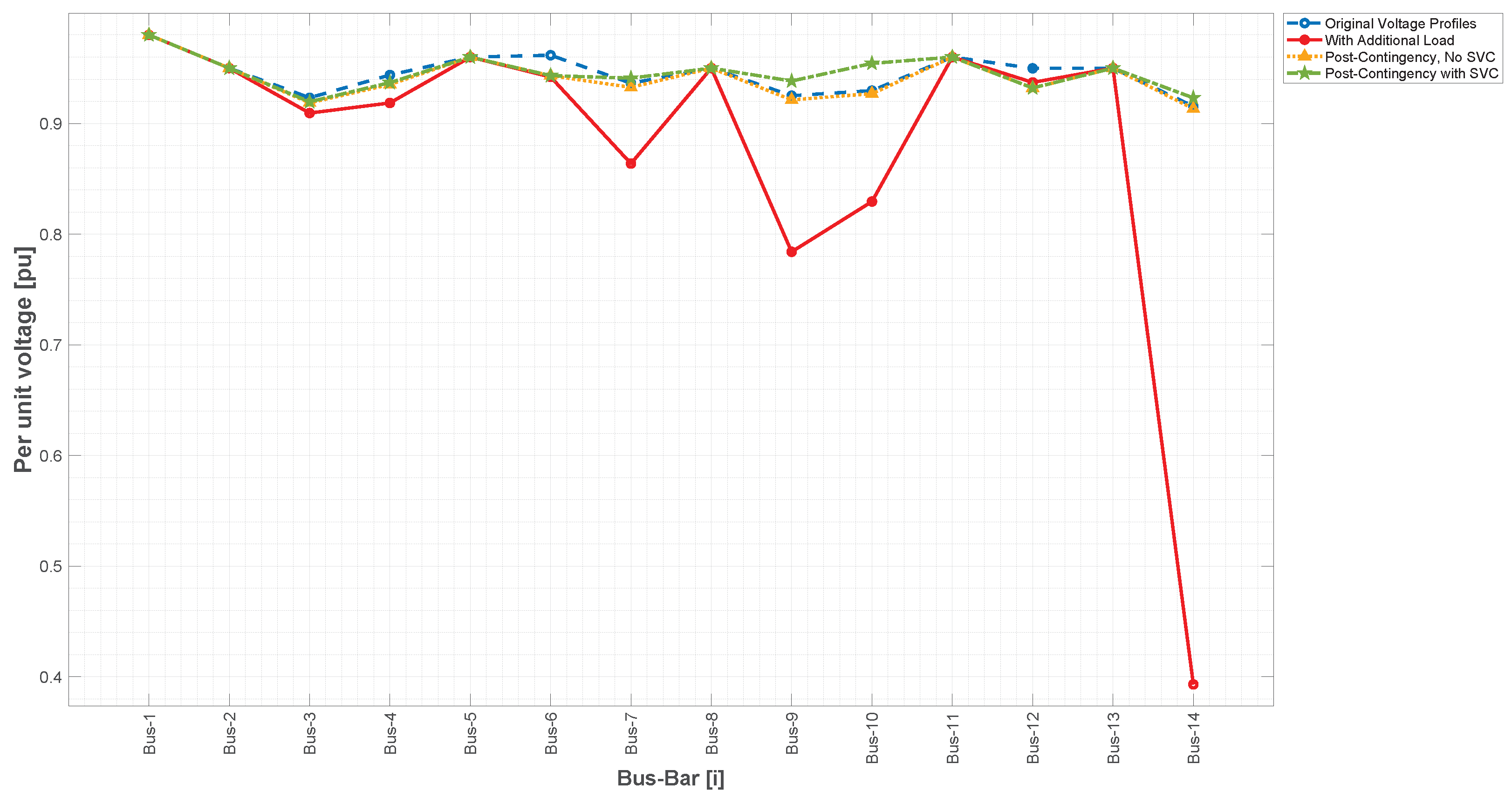
The critical effects of connecting these loads into weak bus bars in the systems are shown in Figure 2, where the voltage profiles are analyzed for the original system and the 10 loading stochastic scenarios.

From Figure 2, it is possible to infer that the average voltage profile in the original system is 0.9453 [pu], with a maximum value of 0.98 [pu] and a minimum of 0.9155 [pu]; then, by analyzing all the loaded cases, the average voltage profile is 0.8799 [pu], with a maximum of 0.98 [pu] and a minimum of 0.3913 [pu]. Therefore, by comparison, the average voltage profile presents a decrease of 6.92%, and the minimum voltage profile decreases as well by 57.26%, with no increase in any case of the voltage profile.

3.1.3. Optimal SVC Location and Sizing

When continuing with the application of Algorithm 4, for every loaded case, the SVC’s optimal sizing and location that will return the FVSI to their original values or improve them are found. For all the analyzed cases, the algorithm gave a unique solution of a single SVC of 25 MVar to be located at bus bar 10. With this solution, the comparison between the loaded cases and their respective case with an SVC is shown in Figure 3. In this analysis, by considering all SVC-compensated cases, the average voltage profile is 0.9452 [pu], with a maximum of 0.98 [pu] and a minimum of 0.8781 [pu]; therefore, when comparing the loaded cases against the compensated ones, the average voltage profile is increased in 7.42% and the minimum in 124.38%.

$${\sigma }_o=\sqrt{\frac{\sum {(x_i-1)}^2}{N}}$$

(8)

Additionally, as Figure 3 shows, all voltage profiles in the compensated scenarios are close to each other with a small deviation. The objective deviation, a formulation that calculates the deviation against one per unit [23], will be used to fully calculate this value. By applying Equation (8), the objective deviation for the original voltage profiles is 0.057243, while the average for the objective deviations of all loaded cases is 0.188785, and the average for the objective deviations of all compensated cases is 0.058073, which shows that the deviation is almost equal to the original scenario. All the results from this section are fully summarized in

Table 5. Summary of voltage profile analysis and objective deviation for IEEE 14-bus bar system.

Parameter	Original System	Loaded Cases	Compensated Cases	% Change (Loaded vs. Original/ Compensated vs. Loaded)
Average Voltage [pu]	0.9453	0.8799	0.9452	$-6.92$%/+7.42%
Maximum Voltage [pu]	0.98	0.98	0.98	0%/0%
Minimum Voltage [pu]	0.9155	0.3913	0.8781	$-57.26$%/+124.38%
Objective Deviation	0.057243	0.188785	0.058073	+229.38%/$-69.24$%

.

3.1.4. Optimal Solution Validation under $N-1$ Contingency Scenarios

The proposed solution will be tested by creating $N-1$ contingency cases. Any lines containing one of the weak nodes identified in Algorithm 3 will be disconnected in these cases. This test will ensure the system can withstand the disconnection of one of these critical lines and continue functioning as before without any additional load. The validation process will also confirm that the system behaves similarly to how it did in its original state before the critical line was disconnected, thus ensuring its reliability.

As a result, 13 transmission lines have been identified as linked to one of the weak nodes that were previously detected. Therefore, for each of the 10 stochastic loaded scenarios, this research will analyze the possibility of disconnecting 13 transmission lines, resulting in 130 study cases to validate this methodology.

As an example of the results obtained, 1 of the 130 scenarios will be chosen randomly to illustrate the methodology used in this paper. In Figure 4, FVSIs are analyzed. The blue line displays the FVSI of the original system, the red line shows the FVSI for the system with additional loads placed on it, and the orange line indicates the FVSI when the loaded system experienced a contingency. Finally, the green line represents the contingency scenario where a transmission line is disconnected under the additional load and optimal SVC placement.

In the given scenario, the 12th line, $lin{e}_{6–12}$, was disconnected, as shown in Figure 4. To increase the load capacity, bus bars 4, 5, and 6 were selected to bear an additional load of 50 MW and 12.5 MVar. The graph’s green line represents the improved FVSIs obtained from the optimal SVC placement methodology, even under contingency scenarios. The results show that the FVSIs are sometimes better than the ones obtained from the original system, which validates this paper’s methodology.

Continuing with the analysis, Figure 5 shows a statistical analysis in which a boxplot for each scenario is generated. This graph shows that all FVSIs decreased with the proposed solution and are closer to each other with a lower deviation.

Then, for a global analysis of all loaded scenarios and all contingency cases for each scenario of stochastic load added to the system, the average value of all FVSIs for every transmission line has been calculated, and, similarly to the contingency scenario with and without SVC, all average values for every transmission line have been calculated. A summary of these values is shown in

Table 6. FVSI statistics summary.

Case	Mean	Min	Max	Standard Deviation
FVSI original	0.049877	0.00035144	0.13917	0.044913
Stochastic loaded scenarios	0.053124	0.0031631	0.13917	0.043307
Contingencies, no SVC scenarios	0.062323	0.0053017	0.19473	0.052709
Contingencies, with SVC scenarios	0.05392	0.0061847	0.1906	0.048871

. This table provides an overview of the power grid’s stability across various scenarios, highlighting the strategic impact of static VAR compensators (SVCs). Initially, the power grid’s stability, with a mean FVSI of 0.049877, indicates a robust system. The introduction of stochastic placed loads slightly increases the mean FVSI to 0.053124, suggesting a significant impact on stability. However, during contingencies without SVC intervention, the mean FVSI surged to 0.062323 when the critical lines were disconnected, revealing a notable decline in stability, with the maximum FVSI peaking at 0.19473. This underscores the network’s vulnerability under contingency scenarios combined with a loaded system in critical nodes. Conversely, implementing SVCs mitigates this instability, reducing the mean FVSI to 0.05392, making it closer to the baseline and significantly lower than the contingency scenario without SVCs. This demonstrates the methodology’s effectiveness in enhancing power grid resilience, particularly by improving stability in the most challenging conditions.

Continuing with the analysis, in Figure 6, voltage profiles are analyzed following the same parameters and color placement as in the FVSI analysis. By considering the same line disconnected as before, the graph indicates that the green line represents the improved voltage profiles obtained from the optimal SVC placement methodology, even under contingency scenarios, having even better voltage profiles than in the original scenario; this once again validates the methodology.

Figure 7 shows the statistical analysis in which each scenario generates a boxplot for the voltage profiles. This figure shows that all voltage profiles are increased, and the deviation for each one is decreased with the optimal solution, even under contingency scenarios.

Similarly, as with the FVSI, a global analysis is performed for the voltage profiles for all loaded scenarios and all contingency cases. A summary of these values is shown in

Table 7. Statistical analysis of voltage profiles.

Scenario	Mean Voltage [pu]	Minimum Voltage [pu]	Maximum Voltage [pu]	Standard Deviation
Original Profiles	0.94537	0.91553	0.98	0.017751
Loaded Scenarios	0.87928	0.39318	0.98	0.15098
Contingencies no SVC	0.93682	0.86778	0.98	0.027156
Contingencies with SVC	0.94157	0.86926	0.98	0.025273

. This table gives an overview of the power grid’s stability across various scenarios by focusing on voltage profiles. Initially, the power grid showcases robust stability, with a mean voltage of 0.94537 [pu] in the original profile. However, the mean voltage drops under loaded scenarios to 0.87928 [pu], with a significant dip in the minimum voltage to 0.39318 [pu], indicating stress under increased load.

Introducing contingencies without SVCs slightly diminishes the mean voltage to 0.93682 [pu], yet the power grid remains relatively stable. Deploying the optimal SVC following this paper’s methodology in response to contingencies significantly improves stability, elevating the mean voltage to 0.94157 [pu], which is close to the system’s characteristics even before the additional loads were connected. Nevertheless, the standard deviation was reduced when the contingencies happened, highlighting SVCs’ critical role in enhancing network resilience against disturbances.

3.2. Case Study: IEEE 30-Bus Bar System

3.2.1. Weakest Power Line by Analyzing $N-1$ Contingency Scenarios

The IEEE 30-bar system consists of 41 transmission lines, which will provide a medium-sized transmission system compared to the previous study case to test this paper’s methodology further. Thus, in this analysis, each possible contingency was executed when disconnecting each line; 41 power line disconnection scenarios were analyzed. Each analysis returned FVSI values for each line, as seen in the example in

Table 8. Example of FVSI at IEEE 30 when $lin{e}_{6–10}$ is disconnected.

Transmission Line		FVSI	Transmission Line		FVSI
Sending Node $\mathit{i}$	Receiving Node $\mathit{j}$		Sending Node $\mathit{i}$	Receiving Node $\mathit{j}$
2	5	0.1952	12	13	0.1170
9	11	0.1569	24	25	0.1032
2	6	0.1256	9	10	0.0913
5	7	0.0768	2	4	0.0716
1	3	0.0661	25	26	0.0581
27	29	0.0469	12	16	0.0448
12	15	0.0442	6	8	0.0437
4	6	0.0407	27	30	0.0373
6	9	0.0365	10	21	0.0326
25	27	0.0324	10	20	0.0302
12	14	0.0292	1	2	0.0287
10	22	0.0286	6	7	0.0267
15	18	0.0257	15	23	0.0253
8	28	0.0242	16	17	0.0230
4	12	0.0197	6	28	0.0191
3	4	0.0144	10	17	0.0131
14	15	0.0126	23	24	0.0110
29	30	0.0108	18	19	0.0091
22	24	0.0090	19	20	0.0080
21	22	0.0036	28	27	0.0025

, in which power $lin{e}_{6–10}$ was disconnected.

Then, by applying Algorithm 2, it was found that the most repeated lines under this analysis (higher FVSIs) were the weakest when it came to cases of instability based on the FVSI.

Table 9. FVSI average value, count, and percentage for selected nodes for all $N-1$ contingencies, IEEE 30-bus bar system.

Power Line		FVSI AvgValue	Count	Percentage [%]
Node $\mathit{i}$	Node $\mathit{j}$
2	5	0.195187059	38	92.68292683
1	3	0.72839528	1	2.43902439
6	10	0.244122555	1	2.43902439
9	11	0.138418004	1	2.43902439

shows the percentage results and the average FVSI value obtained from the line when it was detected as the weakest.

Based on these results, in 92% of the contingency scenarios, $lin{e}_{2–5}$ is the weakest, and based on this, it will be taken as a starting point that sending node 2 and receiving node 5 will be the weakest nodes for the subsequent analysis of this work.

3.2.2. Overloading of Critical Nodes

By applying Algorithm 3 to the previous results, all the associated nodes nearby through a single power line connection with the weakest nodes (2 and 5) were found. Considering that the algorithm discards PV buses and the slack bus, the weak buses identified were bus bars 2, 3, and 4.

Based on [22], the highest load connected in the IEEE 30-bus bar system is 94 MW and node 5, and therefore, by performing multiple power flow analyses, it was found that this maximum load can be increased up to 190%. Thus, 200 MW will be taken as the additional load to be connected to the system.

The maximum load of 200 MW will be stochastically distributed between at least 50% of the previously detected weakest nodes. As in the previous study case, the load will comprise 80% active power and 20% reactive power with 10 cases for stochastic load distribution; thus, the algorithm proposed will be validated under all possible and extreme scenarios.

Table 10. Example of stochastic distribution of additional load for IEEE 30-bus bar system.

Node	Additional Load [MW]	Active Power 80% [MW]	Reactive Power 20% [MVar]
4	80	64	16
2	120	96	24

Total additional load: 200 MW (active: 160 MW, reactive: 40 MW).

shows an example of one case scenario to exemplify stochastic load distribution.

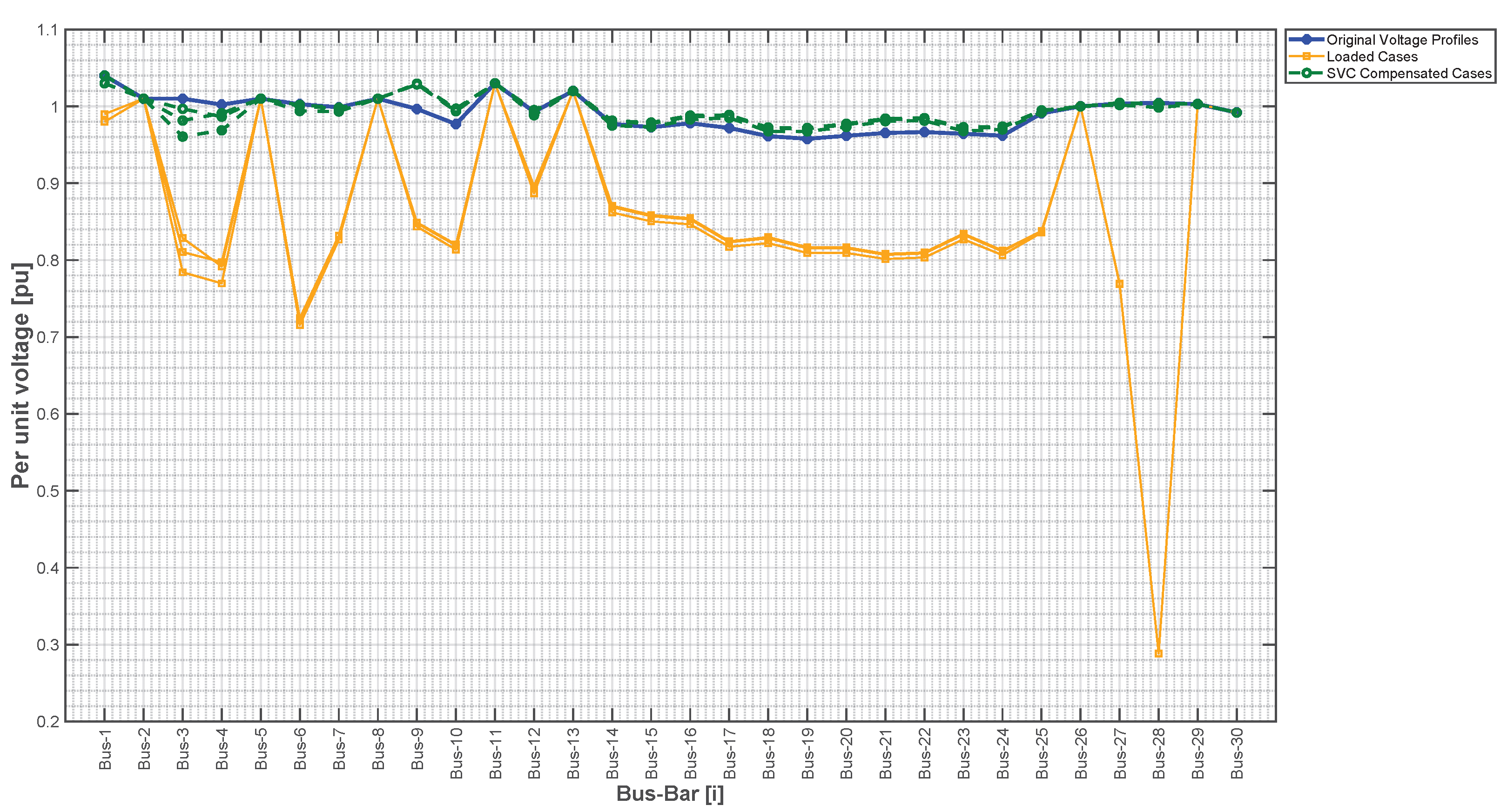
The critical effects of connecting these loads into weak bus bars in the systems are shown in Figure 8, where the voltage profiles are analyzed for the original system and the 10 loading stochastic scenarios.

From Figure 8, it is possible to infer that the average voltage profile in the original system is 0.9911 [pu], with a maximum value of 1.04 [pu] and a minimum of 0.9578 [pu]; then, by analyzing all the loaded cases, the average voltage profile is 0.8596 [pu], with a maximum of 1.03 [pu] and a minimum of 0.2882 [pu]. Therefore, by comparison, the average voltage profile presents a decrease of 13.27%, the minimum voltage profile decreases by 69.90%, and even the maximum voltage profile decreases by 0.9615%.

3.2.3. Optimal SVC Location and Sizing

Applying Algorithm 4 to every loaded case, the SVC’s optimal sizing and location that will return the FVSIs to their original values or improve them are found. For all the analyzed cases, the algorithm gave a unique solution (SVC) of a 45 MVar to be located at bus bar 9.

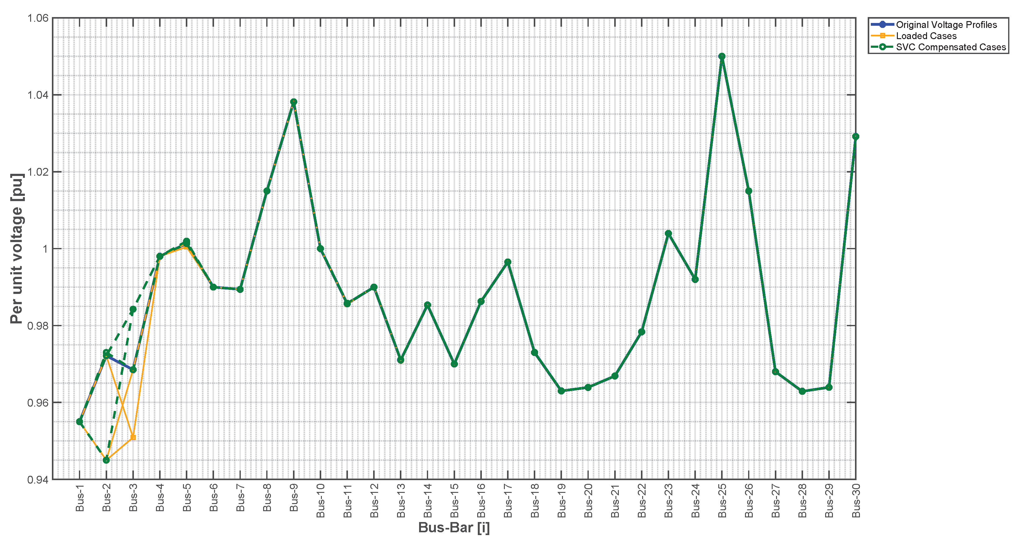
Figure 9 compares the loaded cases and their respective cases with SVC compensation. By considering all SVC-compensated cases, the average voltage profile is 0.9952 [pu], with a maximum of 1.04 [pu] and a minimum of 0.9607 [pu]; therefore, when comparing the loaded cases against the compensated ones, the average voltage profile is increased in 15.77%, the minimum in 233.24%, and the maximum in 0.97%.

Additionally, as Figure 9 shows, all voltage profiles in the compensated scenarios are close with a slight deviation. By applying Equation (8), the objective deviation for the original voltage profiles is 0.0233, while the average for the objective deviations of all loaded cases is 0.1973. The average for the objective deviations of all compensated cases is 0.0187, which shows that the deviation is even lower than in the original system, which emphasizes the methodology’s effectiveness. All the results from this section are fully summarized in

Table 11. Summary of voltage profile analysis and objective deviation for IEEE 30-bus bar system.

Parameter	Original System	Loaded Cases	Compensated Cases	% Change (Loaded vs. Original/ Compensated vs. Loaded)
Average Voltage [pu]	0.9911	0.8596	0.9952	$-13.27$%/+15.77%
Maximum Voltage [pu]	1.04	1.03	1.04	$-0.9615$%/+0.97%
Minimum Voltage [pu]	0.9578	0.2882	0.9607	$-69.9$%/+233.24%
Objective Deviation	0.02339	0.1973	0.01874	+743.82%/$-90.51$%

.

3.2.4. Optimal Solution Validation under $N-1$ Contingency Scenarios

Similar to the 14-bus bar system, the solution will be tested by creating N-1 contingency cases. Any lines containing one of the weak nodes identified in Algorithm 3 will be disconnected in these cases.

As a result, eight transmission lines have been identified as linked to one of the weak nodes that were previously detected. Therefore, for each of the ten stochastic loaded scenarios, this research will analyze the possibility of disconnecting eight transmission lines, resulting in 80 study cases to validate this methodology.

One of the eighty scenarios will be chosen randomly to illustrate the methodology used in this paper. In Figure 10, the same colors as in the previous study case have been selected.

In the given scenario, the fourth line $lin{e}_{3–4}$ was disconnected, as shown in Figure 10. To increase the load capacity, bus bars 2 and 4 were selected to bear an additional load of 100 MW and 25 MVar. The green line shows that the FVSIs are improved due to the optimal SVC placement methodology, even under contingency scenarios. Also, these results show that the FVSIs are sometimes better than the ones obtained from the original system, which validates this paper’s methodology.

Figure 11 shows the statistical analysis in which a boxplot for each scenario is generated. This graph shows that all FVSIs decreased with the proposed solution and are closer to each other with a lower deviation.

Following the corresponding global analysis for all loaded scenarios and all contingency cases performed, for each scenario of stochastic load added to the system, the average value of all FVSIs for every transmission line has been calculated. Similarly, for the contingency scenarios with and without SVC, all average values for every transmission line have been calculated. A summary of these values is shown in

Table 12. FVSI statistics summary for IEEE 30-bus system.

Case	Mean	Min	Max	StdDev
FVSI original	0.044331	0.0035763	0.19519	0.04161
Stochastic loaded scenarios	0.046021	0.0035153	0.19519	0.043612
Contingencies, no SVC scenarios	0.054047	0.0034813	0.19519	0.048011
Contingencies, with SVC scenarios	0.048062	0.0011364	0.19519	0.048058

.

This table provides an overview of the power grid’s stability across various scenarios, highlighting the strategic impact of static VAR compensators (SVCs). Initially, the system shows strong stability with a mean FVSI of 0.044331. Introducing stochastic loads slightly increases the mean FVSI to 0.046021, indicating a minor impact on stability. However, N-1 contingencies without SVC significantly raise the mean FVSI to 0.054047, highlighting the increased system vulnerability. Remarkably, incorporating SVCs during contingencies lowers the mean FVSI to 0.048062, demonstrating SVCs’ effectiveness in enhancing system resilience against disturbances. This analysis underscores the importance of SVCs in maintaining system stability under various operational challenges.

Continuing with the analysis, in Figure 12, voltage profiles are analyzed following the same parameters and color placement as in the FVSI analysis. By considering the same line being disconnected as before, the graph indicates that the green line represents the improved voltage profiles obtained from the optimal SVC placement methodology, even under contingency scenarios, having even better voltage profiles than in the original scenario. This once again validates the methodology.

Figure 13 shows a statistical analysis in which each scenario generates a boxplot for the voltage profiles. This figure shows that all voltage profiles are increased, and the deviation for each one is decreased with the optimal solution, even under contingency scenarios.

Similarly to the FVSI, a global analysis was performed for the voltage profiles for all loaded scenarios and all contingency cases. A summary of these values is shown in

Table 13. Statistical analysis of voltage profiles for IEEE 30-bus system.

Scenario	Mean Voltage [pu]	Minimum Voltage [pu]	Maximum Voltage [pu]	StdDev
Original Profiles	0.99111	0.95779	1.04	0.022005
Loaded Scenarios	0.85958	0.28839	1.03	0.14103
Contingencies No SVC	0.98321	0.94933	1.03	0.0242
Contingencies with SVC	0.99265	0.96625	1.03	0.019131

. This table underscores the critical role of the optimal SVC sized and located through this paper’s methodology. The original system’s mean voltage profile stands at 0.99111 [pu], which experiences a significant dip to 0.85958 [pu] under loaded conditions, underscoring the system’s vulnerability to load variations. However, introducing SVCs remarkably elevates the mean voltage profile to 0.99265 [pu] in compensated scenarios, surpassing even the original system’s stability levels. This enhancement is further evidenced by the substantial reduction in standard deviation from 0.14103 in loaded scenarios to 0.019131 in SVC-compensated scenarios, indicating a more uniform and stable voltage profile across the power grid. The data unequivocally demonstrate the efficacy of SVCs in improving system resilience and ensuring operational stability even under adverse conditions.

3.3. Case Study: IEEE 118-Bus Bar System

3.3.1. Weakest Power Line by Analyzing $N-1$ Contingency Scenarios

Finally, the IEEE 118-bus bar system was selected as the third case study. This system consists of 186 transmission lines, providing an even more complex case study than the previous ones, and further verifying this paper’s methodology. Subsequently, each possible contingency was executed when disconnecting each line; 186 power line disconnection scenarios were analyzed. Each analysis returned FVSI values for each line, as seen in the example in

Table 14. Example of FVSI at IEEE 118 when $lin{e}_{11–12}$ is disconnected.

Transmission Line		FVSI	Transmission Line		FVSI
Sending Node $\mathit{i}$	Receiving Node $\mathit{j}$		Sending Node $\mathit{i}$	Receiving Node $\mathit{j}$
92	100	0.2102	38	65	0.0772
26	30	0.2015	75	77	0.0761
65	66	0.1871	54	59	0.0753
62	66	0.1641	62	67	0.0748
76	77	0.1558	89	92	0.0745
32	113	0.1477	49	51	0.0726
9	10	0.1477	96	97	0.0715
80	96	0.1451	8	30	0.0710
26	25	0.1447	42	49	0.0683
49	54	0.1430	89	90	0.0668
92	94	0.1293	45	49	0.0658
49	54	0.1261	93	94	0.0648
23	25	0.1237	66	67	0.0624
79	80	0.1135	15	17	0.0622
94	100	0.1092	1	2	0.0618
30	17	0.1077	70	75	0.0590
38	37	0.1043	83	85	0.0580
100	101	0.1043	103	104	0.0571
49	69	0.1038	92	93	0.0566
86	87	0.1030	14	15	0.0564
110	112	0.0978	33	37	0.0563
77	80	0.0977	100	104	0.0561
17	31	0.0943	43	44	0.0541
19	34	0.0924	2	12	0.0539
77	82	0.0907	89	92	0.0532

, in which power $lin{e}_{11–12}$ was disconnected. Consider that, due to the high number of power lines, only the first 40 transmission lines are included in the table.

Then, by applying Algorithm 2, it was found that the most repeated lines under this analysis (higher FVSIs) were the weakest when it came to cases of instability based on the FVSI.

Table 15. FVSI average value, count, and percentage for selected nodes for all $N-1$ contingencies, IEEE 118-bus bar system (updated).

Power Line		FVSI AvgValue	Count	Percentage [%]
Node $\mathit{i}$	Node $\mathit{j}$
92	100	0.210239	181	97.31
1	2	0.248576	1	0.54
26	30	0.228579	3	1.61
38	65	0.286559	1	0.54

shows the percentage results and the average FVSI value obtained from the line when it was detected as the weakest.

Based on these results, in 97% of the contingency scenarios, $lin{e}_{92–100}$ is the weakest, and based on this, it will be taken as a starting point that sending node 92 and receiving node 100 will be the weakest nodes for the subsequent analysis of this work.

3.3.2. Overloading of Critical Nodes

By applying Algorithm 3 to the previous results, all the nodes nearby that were associated through a single power line connection with the weakest nodes (92 and 100) were found. Considering that the algorithm discards PV buses and the slack bus, the weak buses identified were bus bars 2, 3, and 12.

Based on [22], the highest load connected in the IEEE 118-bus bar system is 130 MW and node 80, and therefore, by performing multiple power flow analyses, it was found that this maximum load can be increased by up to 180%. Thus, 230 MW will be taken as the additional load to be connected to the system. This maximum load will be distributed among the weakest nodes, as previously established in other study cases.

The critical effects of connecting these loads into weak bus bars in the systems are shown in Figure 14, where the voltage profiles are analyzed for the original system and the 10 loading stochastic scenarios. This figure only shows the first 30 bus bar voltage profiles due to the high number of buses.

By analyzing data from Figure 14, it is possible to infer that the average voltage profile in the original system is 0.98795 [pu], with a maximum value of 1.05 [pu] and a minimum of 0.95 [pu]; then, by analyzing all the loaded cases, the average voltage profile is 0.98154 [pu], with a maximum of 1.05 [pu] and a minimum of 0.4064 [pu]. Therefore, by comparison, the average voltage profile presents a decrease of 0.65%, and the minimum voltage profile decreases by 57.21%.

3.3.3. Optimal SVC Location and Sizing

Applying Algorithm 4 to every loaded case, the SVC’s optimal sizing and location that will return the FVSIs to their original values or improve them are found. For all the analyzed cases, the algorithm gave a unique SVC of 125 MVar to be located at bus bar 3.

Figure 15 compares the loaded cases and their respective cases with SVC compensation. Due to the high number of bars, this graph only illustrates the first 30 bus bars. By considering all SVC-compensated cases, the average voltage profile is 0.9880 [pu], with a maximum of 1.05 [pu] and a minimum of 0.9450 [pu]; therefore, when comparing the loaded cases against the compensated ones, the average voltage profile is increased in 0.65% and the minimum in 132.53%.

By applying Equation (8), the objective deviation for the original voltage profiles is 0.0255, while the average for the objective deviations of all loaded cases is 0.06316. The average for the objective deviations of all compensated cases is 0.0255, which shows that the deviation is equal to the original system, which emphasizes the methodology’s effectiveness. All the results from this section are fully summarized in

Table 16. Summary of voltage profile analysis and objective deviation for IEEE 118-bus bar system.

Parameter	Original System	Loaded Cases	Compensated Cases	% Change (Loaded vs. Original / Compensated vs. Loaded)
Average Voltage [pu]	0.98795	0.98154	0.9880	$-0.649$%/+0.6597%
Maximum Voltage [pu]	1.05	1.05	1.05	0%/0%
Minimum Voltage [pu]	0.95	0.4064	0.9450	$-57.22$%/+132.52%
Objective Deviation	0.0255	0.0631	0.0255	+147.45%/$-147.45$%

.

3.3.4. Optimal Solution Validation under $N-1$ Contingency Scenarios

Similar to the previous cases, the solution will be tested by creating $N-1$ contingency cases. Any lines containing one of the weak nodes identified in Algorithm 3 will be disconnected in these cases.

As a result, ten transmission lines have been identified as linked to one of the weak nodes that were previously detected. Therefore, for each of the 10 stochastic loaded scenarios, this research will analyze the possibility of disconnecting 10 transmission lines, resulting in 100 study cases to validate this methodology.

Given the nature and complexity of this system, only the global analysis will be performed. For each scenario of stochastic load added to the system, the average value of all FVSIs for every transmission line has been calculated; similarly, for the contingency scenarios with and without SVC, all average values for every transmission line have been calculated. A summary of these values is shown in

Table 17. FVSI statistics summary for IEEE 118-bus system.

Case	Mean	Min	Max	StdDev
FVSI original	0.047368	0.00021428	0.21024	0.041701
Stochastic loaded scenarios	0.047675	0.00021428	0.21024	0.042505
Contingencies, NO SVC scenarios	0.047852	0.00021428	0.21024	0.04234
Contingencies, with SVC scenarios	0.047638	0.00021428	0.21024	0.041679

.

This table shows that the mean FVSI values across different scenarios—original, general, contingency, and with SVC implementation—hover around the 0.047 mark, with marginal fluctuations, indicating a consistent system stability profile. Notably, the introduction of SVCs slightly adjusts the mean FVSI to 0.047638 from the original 0.047368, a subtle yet significant enhancement reflecting the SVC’s efficacy in mitigating voltage instability risks. The standard deviation values are minimal across all scenarios, particularly those of the original and SVC-enhanced scenarios (0.041701 and 0.041679, respectively). This analysis, grounded in precise statistical metrics, highlights the critical role of SVCs in maintaining optimal system performance, even as it navigates the acceptable margins between stability thresholds.

Following the same logic, a global analysis is necessary to evaluate the methodology’s performance for all loaded scenarios and all contingency cases in voltage profiles. Similarly, as with the FVSI, a global analysis is performed. A summary of these values is shown in

Table 18. Statistical analysis of voltage profiles for IEEE 118-bus system.

Scenario	Mean Voltage [pu]	Minimum Voltage [pu]	Maximum Voltage [pu]	StdDev
Original Profiles	0.98796	0.95	1.05	0.022585
Loaded Scenarios	0.98154	0.40641	1.05	0.060648
Contingencies No SVC	0.98754	0.94104	1.05	0.023078
Contingencies with SVC	0.98788	0.95	1.05	0.022688

. The system initially shows strong voltage levels, with an average voltage of 0.98796 [pu]. These levels slightly decrease when the system is under a heavy load, but this shows that the system can handle extra loads well. However, some nodes or lines may be vulnerable under stress, as evidenced by the significant drop in minimum voltage to 0.40641 [pu]. Fortunately, the implementation of SVCs improves system stability. The average voltage increases slightly to 0.98788 [pu], which helps mitigate the negative effects of increased loads and keeps the system running smoothly. The standard deviation across scenarios shows that the system performs consistently, and SVC compensation improves voltage uniformity across the power grid. This analysis confirms that SVCs effectively increase voltage stability, particularly in addressing the impact of increased loads and ensuring that the IEEE 30-bus system runs reliably.

4. Conclusions

This paper proposes an approach to efficiently identify the weakest transmission line in an electrical power system. The approach involves analyzing all possible contingency scenarios by disconnecting a transmission line and calculating the FVSI for every remaining transmission line. Based on the results of different cases, the approach proved efficient. For the IEEE 14-bus system, $lin{e}_{2–5}$ was identified as the weakest in 75% of the scenarios. In the IEEE 30-bus system, line $lin{e}_{2–5}$ was identified as the weakest in 92% of the scenarios. Finally, in the IEEE 118-bus system, $lin{e}_{92–100}$ was recognized as the weakest in 97% of the scenarios. Based on this paper’s insights, this identification can help power grid operators improve the EPS’s management.

This paper proposes the optimal placement and sizing of a single static VAR compensator (SVC). This strategy is functional and cost-efficient as it improves the system’s reliability in scenarios where loads are distributed among weak nodes in the transmission systems, which is considered the worst-case scenario for system reliability. To demonstrate the effectiveness of this strategy, the methodology was tested on three different study cases, each with increasing size and complexity. For example, the results of the IEEE 30-bus system were remarkable, with the introduction of a single SVC of 45 MVar at bus bar 9, resulting in a significant improvement in the average voltage profile. The voltage profile, which presented a decrease of 13.27% in loaded scenarios, showed an increase of 15.77% in compensated scenarios. The results were also consistent with the other study cases, which validates the proposed method.

In the case of the IEEE 30-bus system, introducing stochastic loads slightly increases the mean FVSI to 0.046021. This indicates a minor impact on stability. However, $N-1$ contingencies without SVCs significantly raise the mean FVSI to 0.054047. This highlights the increased vulnerability of the system. Incorporating a single SVC during contingencies lowers the mean FVSI to 0.048062. The system’s vulnerability is significantly highlighted under $N-1$ contingencies without SVC, with a 17.44% increase in the mean FVSI. However, implementing SVCs during such contingencies effectively enhances system resilience, reducing the mean FVSI increase to 11.08%. Therefore, the methodology also improves the system stability parameters analyzed. Also, these results are consistent in the other study cases.

The methodology described in this paper demonstrates that the system can efficiently handle additional loads, particularly in nodes identified as critical through FVSI analysis. The system maintains its operational integrity and stability by stochastically distributing additional loads and compensating with a single SVC. For instance, in the third study case of the IEEE 118-bus system, despite a significant increase in load (up to 230 MW), the optimal placement of the SVC ensured that the average voltage profile and system stability were preserved and even improved, highlighting the system’s robustness in accommodating load increments.

The methodology’s effectiveness has been appropriately validated across varying complexity and size systems, ranging from the minor 14-bus system to the extensive and more complex 118-bus system. Its scalability and adaptability have been underscored, proving its utility in real-world applications. With a simple and cost-efficient solution, it offers a reliable approach to enhancing power system stability, optimizing load distribution, and ensuring the operational efficiency of power grids of diverse sizes and configurations.

5. Future Work and Challenges

Future researchers are encouraged to study the optimization of static VAR compensator (SVC) placement and sizing to be analyzed under a broader range of power grid-changing configurations and various operational scenarios. This would include exploring the integration of renewable energy sources and assessing the impact of their inherent variability on the system’s stability. In addition, priority should be given to developing dynamic SVC allocation algorithms that can adapt to real-time changes in the power grid conditions, for instance, when loads are connected to the system and suddenly increase or decrease over time. Therefore, a non-steady state of the system should be studied under those conditions.

By exploring these factors, it will be possible to enhance the resilience of power systems against increasingly complex and unpredictable operational challenges, ensuring reliability and stability in the face of shifting load demands and generation capacities.

References

- Gupta, S.K.; Mallik, S.K. Enhancement in Voltage Stability Using FACTS Devices Under Contingency Conditions. J. Oper. Autom. Power Eng. 2024, 12, 365–378. [Google Scholar] [CrossRef]
- Hosseinzadehtaher, M.; Zare, A.; Khan, A.; Umar, M.F.; D’silva, S.; Shadmand, M.B. AI-Based Technique to Enhance Transient Response and Resiliency of Power Electronic Dominated Grids via Grid-Following Inverters. IEEE Trans. Ind. Electron. 2024, 71, 2614–2625. [Google Scholar] [CrossRef]
- Basha, M.I.; Eldesouky, A.A. Multi-objective-based reactive power planning and voltage stability enhancement using FACTS and capacitor banks. Electr. Eng. 2022, 104, 3173–3196. [Google Scholar] [CrossRef]
- Singh, R.K.; Singh, N.K. Power system transient stability improvement with FACTS controllers using SSSC-based controller. Sustain. Energy Technol. Assess. 2022, 53, 102664. [Google Scholar] [CrossRef]
- Tina, G.M.; Maione, G.; Licciardello, S.; Stefanelli, D. Comparative Technical-Economical Analysis of Transient Stability Improvements in a Power System. Appl. Sci. 2021, 11, 11359. [Google Scholar] [CrossRef]
- Sakipour, R.; Abdi, H. International Journal of Electrical Power and Energy Systems Voltage stability improvement of wind farms by self-correcting static volt-ampere reactive compensator and energy storage. Int. J. Electr. Power Energy Syst. 2022, 140, 108082. [Google Scholar] [CrossRef]
- Ariel, M.; Nwulu, M. Optimal Placement of FACTS Devices Using Filter Feeding Allogenic Engineering Algorithm. Technol. Econ. Smart Grids Sustain. Energy 2022, 7, 2. [Google Scholar] [CrossRef]
- Abdul, A.; Altahir, R.; Marei, M.M. An optimal allocation of UPFC and transient stability improvement of an electrical power system: IEEE-30 buses. Int. J. Electr. Comput. Eng. 2021, 11, 4698–4707. [Google Scholar] [CrossRef]
- Azbe, V.; Mihalic, R. International Journal of Electrical Power and Energy Systems STATCOM control strategies in energy-function-based methods for the globally optimal control of renewable sources during transients. Int. J. Electr. Power Energy Syst. 2022, 141, 108145. [Google Scholar] [CrossRef]
- Balakumar, S.; Getahun, A.; Kefale, S.; Kumar, K.R. Improvement of the Voltage Profile and Loss Reduction in Distribution Network Using Moth Flame Algorithm: Wolaita Sodo, Ethiopia. J. Electr. Comput. Eng. 2021, 2021, 9987304. [Google Scholar] [CrossRef]
- Wartana, I.M.; Agustini, N.P.; Sreedharan, S.; Lbs, M. Improved security and stability of grid connected the wind energy conversion system by unified power flow controller. Indones. J. Electr. Eng. Comput. Sci. 2022, 27, 1151–1161. [Google Scholar] [CrossRef]
- Ghaedi, S.; Abazari, S.; Markadeh, G.A. Transient stability improvement of power system with UPFC control by using transient energy function and sliding mode observer based on locally measurable information. Measurement 2021, 183, 109842. [Google Scholar] [CrossRef]
- Vaidya, P.; Chandrakar, V.K. Exploring the Enhanced Performance of a Static Synchronous Compensator with a Super-Capacitor in Power Networks. Eng. Technol. Appl. Sci. Res. 2022, 12, 9703–9708. [Google Scholar] [CrossRef]
- Rasool, A.A.; Abbas, N.M.; Sheikhyounis, K. Determination of optimal size and location of static synchronous compensator for power system bus voltage improvement and loss reduction using whale optimization algorithm. East.-Eur. J. Enterp. Technol. 2022, 1, 26–34. [Google Scholar] [CrossRef]
- Khan, B.; Redae, K.; Gidey, E.; Prakash, O. Optimal integration of DSTATCOM using improved bacterial search algorithm for distribution network optimization. Alex. Eng. J. 2022, 61, 5539–5555. [Google Scholar] [CrossRef]
- He, P.; Pan, Z.; Fan, J.; Tao, Y.; Wang, M. Coordinated design of PSS and multiple FACTS devices based on the PSO-GA algorithm to improve the stability of wind – PV – thermal-bundled power system. Electr. Eng. 2023, 106, 2143–2157. [Google Scholar] [CrossRef]
- Pattabhi, M.B.; Rangappa, B.; Krishna, L.; Sundar, S. A Novel Method for Contingency Ranking Based On Voltage Stability Criteria in Radial Distribution Systems. Technol. Econ. Smart Grids Sustain. Energy 2022, 7, 9. [Google Scholar] [CrossRef]
- Al-wazni, H.S.M.; Al-kubragyi, S.S.A. A hybrid algorithm for voltage stability enhancement of distribution systems. Int. J. Electr. Comput. Eng. 2022, 12, 50–61. [Google Scholar] [CrossRef]
- Djellad, A.; Belakehal, S.; Chenni, R.; Dekhane, A. Reliability improvement in serial multicellular converters based on statcom control. J. Eur. Des Syst. Autom. 2021, 54, 519–528. [Google Scholar] [CrossRef]
- Jaramillo, M.D.; Carrión, D.F.; Muñoz, J.P. A Novel Methodology for Strengthening Stability in Electrical Power Systems by Considering Fast Voltage Stability Index under N-1 Scenarios. Energies 2023, 16, 3396. [Google Scholar] [CrossRef]
- Musirin, I.; Abdul Rahman, T. Novel fast voltage stability index (FVSI) for voltage stability analysis in power transmission system. In Proceedings of the Student Conference on Research and Development, Shah Alam, Malaysia, 17 July 2002; pp. 265–268. [Google Scholar] [CrossRef]
- Jaramillo, M.; Carrión, D.; Muñoz, J. A Deep Neural Network as a Strategy for Optimal Sizing and Location of Reactive Compensation Considering Power Consumption Uncertainties. Energies 2022, 15, 9367. [Google Scholar] [CrossRef]
- Jaramillo, M.; Tipán, L.; Muñoz, J. A novel methodology for optimal location of reactive compensation through deep neural networks. Heliyon 2022, 8, e11097. [Google Scholar] [CrossRef] [PubMed]
Figure 1.
Example of fast voltage stability index calculation in transmission line for a section of the IEEE 14-bus bar transmission system.
Figure 2.
Voltage profiles across IEEE 14-bus system under varied load conditions.
Figure 3.
Voltage stability across buses: original vs. adjusted profiles.
Figure 4.
FVSI dynamics across buses when is disconnected and buses 4, 5, and 6 are loaded.
Figure 5.
Boxplot analysis for FVSI dynamics across buses.
Figure 6.
Voltage profile dynamics across buses when is disconnected and buses 4, 5, and 6 are loaded.
Figure 7.
Boxplot analysis for voltage profile dynamics across buses.
Figure 8.
Voltage profiles across IEEE 30-bus system under varied load conditions.
Figure 9.
Voltage stability across buses: original vs. adjusted profiles in the IEEE 30-bus bar system.
Figure 10.
FVSI dynamics across buses when is disconnected and buses 2 and 4 are loaded.
Figure 11.
Boxplot analysis for FVSI dynamics across buses, IEEE 30-bus bar system.
Figure 12.
Voltage profile dynamics across buses when is disconnected and buses 2 and 4 are loaded.
Figure 13.
Boxplot analysis for voltage profile dynamics across buses, IEEE 30-bus bar system.
Figure 14.
Voltage profiles across IEEE 118-bus system under varied load conditions.
Figure 15.
Voltage stability across buses: original vs. adjusted profiles in the IEEE 118-bus bar system.