1. Introduction
In recent trends, wind turbines have been growing in size, and to manufacture these large turbine blades at a lower cost, they often adopt a lightweight design that compromises their structural rigidity [
1,
2,
3,
4]. The increased flexibility of these up-scaled blades makes them more aeroelastically sensitive to nonuniform atmospheric flow patterns, which inflict fluctuating loads on the rotor plane [
5,
6]. Additionally, wakes from these turbines tend to develop complex structures, which evolve in ways that are difficult to predict as they interact with wind farm flow. These challenging factors necessitate a priority for research that investigates the complex multi-physics response of modern utility-scale wind turbines in naturally variant atmospheric flow conditions [
7,
8]. This research thrust is what we aim to address in this work.
Since modern design changes to the classic wind turbine blade structure have influenced the structural and aeroelastic characteristics of the blade, it is no longer possible to draw accurate conclusions from studies performed on older wind turbines, which were intended to operate at a smaller scale [
9]. It also is not feasible to properly investigate the aerodynamic and structural properties of these large, flexible turbine blades at full scale using wind tunnel testing, because their dimensions have grown larger than the largest wind tunnel facility that is available today [
10]. Wind tunnel testing is only further excluded as an option by the physical difficulties involved with generating scaled-down wind tunnel flow that mimics the variations that are naturally observed in the atmosphere at full scale. Thus, this dynamic relationship between atmospheric variability and large, flexible turbine operation is often studied through computational simulations of wind turbine aeroelastic response and farm fluid flow interactions.
To simulate large-scale wind turbines where the atmospheric flow is highly variant or complex, most numerical methods require an immense computational expense to evaluate high-fidelity solutions of turbine behavior. In general, the enhanced accuracy of numerical simulation usually comes with a higher computational demand, so current wind turbine simulation methods are designed to provide some compromise between computational efficiency and the fidelity of the solution. At one extreme, models that perform the direct numerical simulation of the Navier–Stokes equations prioritize the exactness of the solutions [
11], whereas reduced-order techniques simplify the computations to prioritize efficiency [
12]. Between these extremes, there exists a wide range of simulation tools for wind turbine modeling, such as Reynolds-averaged Navier–Stokes (RANS) techniques [
13,
14,
15,
16] and Large Eddy Simulation (LES) techniques [
17,
18,
19,
20], which tend to be most popular in recent research works despite a somewhat large computational expense [
21,
22]. Custom trade-offs between precision and computational efficiency are made to fit the specific applications of each wind turbine modeling tool. In works such as Burton et al. [
23] and Manwell et al. [
24], simulations of rotor flow and aeroelastic blade behavior are solved through the coupled evaluations of blade structural dynamics and fluid flow interactions at a reduced-order computational cost, by employing custom adaptations to the Blade-Element Momentum (BEM) model.
Introduced and validated in Ponta et al [
25], the
Common Ordinary Differential Equation Framework (
CODEF) employs an advanced adaptation to the BEM technique within a modeling suite of cooperative multi-physics simulation modules, to generate high-fidelity solutions of wind turbine aeroelastic behavior, rotor flow, wind farm fluid flow dynamics, and more, at a moderate computational cost.
CODEF is a uniquely valuable tool for this research because it is capable of simulating large, complex wind turbine operational dynamics for a computational demand that is much less than what is required of typical LES or RANS techniques.
In this work, we use
CODEF to perform a high-fidelity analysis of utility-scale, flexible-bladed turbine operation in realistically variant atmospheric flow conditions. More specifically, we explore how changes to the structural design of modern wind turbine blades influences rotor aeroelastic behaviors and turbine interactions with farm flow. This was investigated via simulations of the Sandia National Labs (SNL) National Rotor Testbed (NRT) turbine, located at the SNL Scaled Wind Farm Technology (SWiFT) facility in Lubbock, TX [
26,
27,
28]. The NRT blade was chosen because it was specifically designed to research the dynamics of large, flexible wind turbine operation at a scaled-down size to reduce associated expenses.
A virtual model of the NRT blade was created using the detailed specifications provided in Kelley [
29], including material data, constructive methods, blade mechanical properties, and turbine control systems. The introduction of the actual material data contained in Kelley’s [
29] report into the input of our model was of crucial importance to ensure that the results of our numerical experiments are reliable. Similar studies on the identification of the mechanical properties of composite materials for aerospace engineering applications could be found in works like Karpenko et al. [
30] and Karpenko and Nugaras [
31].
Flexible variations of this baseline NRT blade were created by reducing blade materials to 60%, 40%, and 20% of their original thicknesses. By doing this, we intentionally exacerbated the flexible characteristics, which make large rotors sensitive to the fluctuating aerodynamic loads introduced by variant atmospheric flow conditions, in order to study the corresponding effects.
These NRT flexible variations were simulated with several scenarios representing typical wind conditions observed at the SWiFT facility, by sampling field measurements from on-site meteorological towers to create multiple types of wind inputs. We used three inputs to model and explore the role of atmospheric spatiotemporal variance in the dynamics of wind turbine and wind farm flow interactions. The wind scenarios simulated in this study range from a simple Steady-In-The-Average (SITA) flow state, to realistic time evolutions of measured flow conditions.
In this paper, we present solutions of rotor aeroelastic simulation and wind farm flow visualizations of wake vorticity and velocity, to analyze the observed effects caused by changes in blade flexibility and atmospheric flow fluctuations in the background wind. A specific focus was given towards identifying the nature and extent of the aeroelastic sensitivities of large, flexible rotors to variant wind inflow conditions, and elucidating how differences in turbine and vortex wake interactions with various atmospheric flow states yield discernible changes to the structures of the turbine’s wake.
In order to facilitate the interpretation of the abbreviations and acronyms used in this work, a table has been added to the Abbreviations Section at the end of the paper.
2. Theoretical Background and Methodology
In this section, we provide a concise overview of the Common ODE Framework (CODEF) to elucidate its applications for the simulation of wind turbine and farm flow dynamics. In the scope of this paper, we employed the capacities of CODEF to assess the solutions of the blade structure, aeroelastic rotor response, and wind farm flow vortex interactions.
CODEF is a wind turbine modeling tool that is comprised of a suite of inter-related modules, which all interface with a central Ordinary Differential Equation (ODE) solver. Each module imposes governing equations and boundary conditions to define the multi-physics principles of turbine and farm-level dynamics, such as wind turbine and farm controls, rotor and farm flow, atmospheric characterization, blade structure deformation, and more. The calculative processes of the variable-order ODE solver are guided by the definitions imposed by each of these modules. Thus, the ODE solver integrates elements from all modules in the framework collectively, in adaptive time-iterative steps, to reach a solution at each time step. At each succession in time, the local truncation error is regulated to maintain the sequential time-marching of CODEF computations in a stable, time-efficient manner.
The following subsections summarize various subroutines of
CODEF, including their theoretical basis and other characteristics that pertain to the subject of this research. Further information regarding
CODEF’s aeroelastic modules and validation tests are described to depth in Ponta et al. [
25].
2.1. Model for Turbine Blade Structure and Aeroelastic Response
To model turbine aeroelastic behavior in
CODEF, an advanced variation of the classic Blade Element Momentum (BEM) approach is implemented to evaluate rotor flow dynamics. In the classic BEM method, an idealized two-dimensional actuator disk represents the turbine rotor, and all fluid flow that passes through this actuator disk is contained within a theoretical stream-tube. Aerodynamic forces are calculated by evaluating the change in momentum as fluid passes through the idealized actuator disk. Although this original formulation of the BEM model does not account for time-dependent changes to blade shape within the rotor plane, the adapted BEM approach implemented in
CODEF achieves a more robust characterization of rotor flow. With information supplemented from the structural solutions of blade section deformations during turbine operation, the
CODEF Dynamic Rotor Deformation-Blade Element Momentum (DRD-BEM) model has the capacity to represent the transient shape changes of the rotor, and the cascading effects on aeroelastic responses [
25].
The DRD-BEM model is formed from the coupling of the structural blade model and the adapted BEM calculations. The structural model includes a variation of the Generalized Timoshenko Beam Model (GTBM), which acts to reduce the three-dimensional analysis of the blade structure into time-dependent, one-dimensional nonlinear evaluations of previously resolved sectional planes along the blade’s span. The GTBM operates in a similar manner to the classical Timoshenko theory, by modeling the wind turbine blade as a beam of equivalent stiffness, through two-dimensional finite-element analyses of cross-sections along the blade’s span [
32]. The
CODEF GTBM differs from the original Timoshenko theory because it does not assume that these cross-sections remain undeformed planes during operation. Instead, the blade’s warping structure is evaluated via interpolations on a two-dimensional mesh, and used to define the three-dimensional strain energy through a 6 × 6 stiffness matrix, which is fully populated in terms of the original Timoshenko theory variables. Through these manipulations, the GTBM successfully exploits dimensional reduction to represent the three-dimensional structural characteristics of the beam at a reduced computational cost.
Additional details about the coupling of DRD-BEM with the structural GTBM can be found in Ponta et al. [
25] and Otero and Ponta [
32], which also include validation tests, and the application of these models to the analysis of the vibrational modes of composite blades.
The DRD-BEM uses the coupled deformation modes produced by the GTBM to guide its evaluation of rotor flow, incorporating changes to blade shape and aerodynamic attitude during operation. This is performed by employing linear operator coordinate transformations to align the incoming wind velocity into the coordinate system of deformed blade sections. To begin this process, the velocity of incoming wind,
, from the simulated ground coordinate system, is transformed into the coordinate system of the rotor hub. Misalignment of the incoming flow relative to the hub is caused by factors such as yaw offset, tilt, and the angle of azimuth, and is accounted for with linear operators
,
, and
, respectively.
Figure 1 shows the manner in which these coordinate transformations are applied in the DRD-BEM module.
Performing the transformations shown in
Figure 1 aligns the BEM annular actuator disk with the coordinate system of the hub, making it possible to evaluate the velocity vector components affected by interference at the rotor. Axial and tangential induction factors,
a and
, are employed in the following equation to solve for the velocity vector,
, representing the wind in the hub coordinate system after it is influenced by interference at the rotor.
Additional linear operators are applied to the wind velocity vector,
, to align with respect to the blade-root coordinate system, by accounting for factors such as coning and pitching using linear operators
and
. The DRD-BEM also interprets solutions from the structural model at this time to accommodate misalignment due to instantaneous changes in blade section configuration, using operators
and
. Additionally, the velocity vector incorporates velocity components from structural vibrations,
, and mechanical actions,
, to evaluate the full characterization of flow relative to each blade section. These calculations are depicted in
Figure 2, showing the process of the accommodations.
The corresponding aerodynamic coefficients of lift and drag are identified based on the inflow angle of attack to evaluate the total aerodynamic load for each blade section element. This load can also be projected back into the hub coordinate system via the reversal of the previously described transformations [
25]. This assessment of aerodynamic load at the blade sections and the hub enables the
CODEF suite to evaluate turbine structural response, fluid flow interactions, wind turbine power output, and more, including information communicated with the other submodules of the framework.
Comprehensive details about the DRD-BEM formulation, and its full mathematical derivation, can be found in Ponta et al. [
25], together with results that were validated against the works of Jonkman et al. [
33] and Xudong et al. [
34], plus the results of the DRD-BEM model applied to the analysis of the vibrational modes of composite laminated wind turbine blades.
Additionally, the use of the DRD-BEM model for the solution of a number of different aeroelastic problems in wind turbine rotors can be found in the following references, among several others. Otero and Ponta [
35] used the model to analyze the effects of blade section misalignment on rotor cyclic loads. Jalal et al. [
36] reported the results of the DRD-BEM model applied to studying the effects of controlled gust pulses on the oscillatory response of wind turbine rotors. Menon and Ponta [
37] analyzed the effects of flap control actions. Rajan and Ponta [
38] studied the rotor’s response in high-aerodynamic-interference conditions.
2.2. Turbine Wake Flow Model
The
CODEF module for farm flow vortex wake simulation has the capacity of modeling inter-turbine wake dynamics and wake interactions with background atmospheric flow, through implementations of the Gaussian-core Vortex Lattice Model (GVLM), introduced in Baruah and Ponta [
39]. The GLVM is an advanced vortex wake model, which is informed by time-dependent aeroelastic blade responses to generate high-fidelity simulations of wind farm flow dynamics at an economized computational cost.
The CODEF GVLM leverages the information from the characterizations of the background fluid flow, and DRD-BEM spanwise evaluations of circulation about blade sections to project the shedding and mutual advection of vortex wake structures downstream of the turbine. These evaluations of the wake structure are later used in this paper to analyze the interactions with the background wind farm flow, and evolving patterns of flow velocity induced at locations in the propagated wake.
In this section, we briefly describe the
CODEF-GVLM only as it pertains to the scope of this paper, in an effort to provide a comprehensive explanation of the model that is succinct. For a more detailed elaboration of the GVLM conceptual basis, the mathematical formulation, and the sequential protocol for vortex-lattice structure generation, the readers are directed to Baruah and Ponta [
39]. This reference also furnishes a series of validation tests comparing GVLM simulations of wind turbine operation at SNL’s SWiFT facility to corresponding LiDAR field measurements of wake velocity patterns from the SWiFT site in Herges et al. [
40].
As discussed later in
Section 2.3, and to a greater depth in Baruah and Ponta [
39], the undisturbed wind farm flow is fully characterized in
CODEF via several input parameters, so that the DRD-BEM model can accurately calculate the instantaneous velocity of incoming wind and the corresponding circulation of flow about the blade sections. With this value of circulation, the GVLM evaluates bound vortex filaments by applying the Kutta–Joukowski lift theorem at all blade section elements [
41]. The vorticity strength of the bound vortex filament changes at each time step with respect to the circulation of flow around the blade element, and thus, the bound vortex filament from the previous time-step is shed at the trailing edge of the blade as the current filament is generated at the quarter chord. As these finite-length vortex filaments are formed at subsequent time-steps of the ODE solver, they are aggregated by the GVLM to construct a vortex-filament lattice, which transmits a detailed representation of the wind turbine’s wake structure as it evolves downstream and interacts with wind farm flow.
The distance traveled by a point in the lattice at an instance in time can be calculated with respect to the fluctuating patterns of velocity in the background wind, and its influence on the advection of the vortex-lattice structure in the wake downstream of the turbine. We can also evaluate the wake’s converse effect on the background wind farm flow velocity patterns through projections of the velocity induced by the wake’s vortex-filament structure, using a custom application of the velocity-induction law for finite-length vortex filaments [
42,
43].
Since the common classical Biot–Savart singularity representation of vorticity is prone to estimating unrealistically high values of velocity at close proximity to the vortex core, the
CODEF-GVLM implementation of this method, as described in Ponta et al. [
25], utilizes Gaussian distributions of vorticity in finite-length vortex-filament cores.
CODEF Gaussian-core adaptations to this technique preclude the issue of extreme projections of induced velocity and, therefore, produce more realistic evaluations of vortex wake-induced velocity patterns in farm flow. Additionally, the Gaussian-core approach provides a more accurate description of viscous decay, compared to simple singularity representations of vorticity, which do not model any diffusion of the vortex core. This enables the
CODEF-GVLM approach to be more computationally efficient, by off-loading calculations for filaments whose vortex cores have sufficiently diffused to have negligible effects.
In this work, will use solutions from the GVLM to examine the structure and evolution of the vortex wake, as it interacts with various fluctuating wind conditions. Using the calculations of tangential velocity induction from vortex filaments in the lattice structure, we will project downstream velocity patterns into the background atmospheric flow. This will serve as an analytic aid to evaluate differences in wake structure and flow dynamics that result from changes in rotor stiffness and background wind.
In the interest of brevity, and to make this paper self-contained, only pertinent details about this model have been described in this section. For more thorough discussions of Gaussian vortex core distributions and methodologies for generating the vortex-filament core, see Ponta [
44], Flór and van Heijst [
45], Trieling et al. [
46], Hooker [
47], and Lamb [
48]. Topics relating free vortex lattice methods, including vortex-filament induction of velocity, are discussed at length in Cottet and Koumoutsako [
49], Strickland et al. [
43], and Karamcheti [
50]. Further elucidation of the implementation, derivation, and validations of the GVLM is provided in Ponta and Jacovkis [
42], Ponta [
44], and Baruah and Ponta [
39].
2.3. Characterization of Atmospheric Flow
Naturally occurring patterns of velocity distributions in atmospheric flow are known to introduce fluctuating aerodynamic loads at the rotor and profound effects on wind farm flow dynamics [
51,
52,
53]. Therefore, the accuracy of the
CODEF solution for farm flow interactions is inherently dependent on the quality of the definition for ambient wind farm flow conditions. To achieve a precise description of this initial state of flow, wind conditions are defined through the assignment of several user input variables, which characterize atmospheric flow variations in space and time.
Ambient atmospheric flow is characterized in CODEF by describing the spatial distributions of inflow qualities at locations at a height above the ground (the z direction) and across the spanwise width of the turbine rotor (the y direction), thus identifying a mean flow profile at each time-step of the ODE solution. Flow variations in the y and z directions are established through the assignment of four primary variables, which quantitatively define the state of undisturbed wind inflow and, when sampled in time, the rates of variation naturally occurring within it. These variables have been well defined and used in the past in a practically universal manner. They include two localized magnitudes, hub-height wind speed and hub-height wind direction, plus two cross-plain defined magnitudes, the exponent of vertical wind shear and the directional veer.
The values of these parameters can be obtained by sampling data collected from wind measurements. Wind speed, , and wind direction, , are defined at the turbine’s hub height. is determined by the speed of undisturbed wind incoming at the hub, expressed in meters per second. The yaw offset of the turbine, , can be found by subtracting the angular alignment of the rotor’s azimuthal axis from , where a positive signifies a positive yaw offset.
can be defined as the variation in the direction of
across the rotor plane in the
z direction. This can be found by finding the angular difference between the wind direction observed at the lowest and highest point of the rotor plane. The exponent
describes the variation in the magnitude of
with respect to locations in the height above the ground,
z (see Manwell et al. [
24] and Burton et al. [
23], among others). The value of
defines the shape of the power law curve for the wind-sheer velocity profile, as shown in the following equation:
where the subscript
refers to values at a reference height, in our case, the hub height.
Spatiotemporal variations in atmospheric flow naturally occur at a variety of scales, and the GVLM module in
CODEF addresses the modeling of smaller-scale fluctuations of wind differently, depending on the relative time-scale of these fluctuations. To illustrate this point,
Figure 3 shows an example of the power spectral density for a typical anemometer sample taken at the SWiFT facility [
54]. As noted in this plot, the larger scale, coherent structures in wind fluctuations are resolved by the vortex-lattice evolution, and introduced into the model via changes in the input of the four wind parameters described above. A symbolic visualization of this concept is provided in
Figure 3a, where a curvilinear wind profile captures the spatial cross-flow variations. These coherent structures can be distinguished from small-scale flow fluctuations, because they are able to persist over a longer duration of time, due to their stronger coherent vorticity content, which distinguishes them from the small-scale high-frequency fluctuation patterns. These coherent vortex structures, therefore, occupy a domain of relatively lower frequency fluctuations, which can be resolved by the GVLM vortex lattice.
Similarly noted in
Figure 3b, the effect from smaller-scale motions in the short-term wind fluctuations are modeled in
CODEF-GVLM via an equivalent Turbulent Diffusivity Coefficient (TDC), which governs the diffusion of vorticity in the Gaussian core of the filaments in the vortex lattice [
39]. In
Figure 3a, the scale of these smaller fluctuations is symbolized by the difference between the “instantaneous wind” and the curvilinear surface designated as “resolved scales’ input”. The latter surface, which also varies in time, but at a lower frequency, represents the variations that the coherent structures induce in the atmospheric wind flow, and the way in which they are introduced in the model.
As was mentioned before, the instantaneous deviations induced by the small-scale fluctuations are modeled in the
CODEF-GVLM suite by the TDC. The TDC can be considered analogous to the kinematic eddy viscosity in traditional sub-grid modeling techniques like LES or RANS. The TDC aims to capture effects from smaller scale, short-term turbulent fluctuations that influence the decay of vorticity in the Gaussian cores and, hence, the dissipation of the wake. The value of the TDC has been calibrated through comparisons of the GVLM results to LiDAR wake velocity measurements [
40,
55], at various levels of turbulence intensity.
To find more details regarding the GVLM representation of wind input parameters in the atmospheric flow velocity profile, and how turbulent atmospheric flow fluctuations are modeled through the TDC, the reader is referred to Baruah and Ponta [
39].
In
Section 4, we present the results from the
CODEF simulations of turbine operation in fluctuating atmospheric conditions measured at the SWiFT facility. As a part of the analysis of the results, these topics are revisited in connection with the spectrum of the atmospheric fluctuations found in the measured anemometry signals, and how they are processed for the
CODEF model input.
3. Controlled Pulse Analysis of the SNL NRT Blade Operating in SITA Wind Profiles
In this section, we explain the methodology of our experimental approach, and analyze the numerical results. Through this work, we aim to assess changes in rotor aeroelastic sensitivity to fluctuations in wind farm flow, in response to the increasing flexibility of lightweight rotor designs found in modern utility-scale turbines. Investigative simulations were performed in a diverse set of atmospheric wind conditions to evaluate the operation of several flexible wind turbine blade variations. The results from these simulations were used to analyze how differences in blade flexibility can affect the aeroelastic behaviors evoked by interactions with fluctuating atmospheric flow, and how these behaviors may shape the vortex structures generated in the propagating wake.
To initiate our analysis, modifications were made to the structural components of the National Rotor Testbed (NRT) wind turbine, generating a series of blades exhibiting varying levels of flexibility. Flexible variations of the NRT blade were created by reducing the spar cap and shell to 60%, 40%, and 20% of the original NRT baseline thickness. See Kelley [
29] for details regarding aspects of the NRT blade’s design, construction, and controls system.
Figure 4 shows several properties of these flexible blade variations, plotted at locations along the blade’s span.
In the context of the experimental design of this study, it is also important to note the capacities at which atmospheric flow variations affect fluctuating aerodynamic loads at the rotor, and the influence that these loads have on wind turbine and collective farm performance. If the turbine is operating in a uniform, steady mean flow profile containing no shear, veer, or yaw offset, the rotor will experience a fairly constant aerodynamic load, but in other cases where a Steady-In-The-Average (SITA) flow state introduces a shear, veer, or yaw offset, the rotor inflow is spatially nonuniform and constant in time. Thus, the turbine will undergo cyclical patterns of aerodynamic loading as the turbine blades rotate through a gradient of wind velocities [
51]. In more realistic scenarios of wind inflow, it is common for non-cyclical aerodynamic loading patterns to emerge as a result of turbine operation in a wind profile that contains turbulence. In this case, spatiotemporal variations in atmospheric flow create a nonuniform flow field, which also fluctuates with time.
To investigate the effects of these differing scenarios of variant wind inflow, the aforementioned flexible variations of the NRT turbine were simulated using CODEF to impose operating conditions that feature three increasingly complex states of flow variance. These three types of simulated conditions are listed below:
Cyclical variations (SITA wind profile): Wind inputs consist of an average value for wind speed, wind direction, and vertical shear, which characterize the spatial variance of background atmospheric flow in height only. Veer was kept at a constant value of
. Input parameters for wind conditions do not change with time. The simulations were conducted at a range of wind speeds, with and without a
yaw offset, and in shear profiles typical of day and night conditions. See the results in
Section 3.1.
SITA with controlled pulses: Wind conditions are similar to SITA, but feature an artificially controlled, short-term increase in wind speed. After the short increase in wind speed, the conditions return to the initial SITA conditions. The simulations were conducted at two wind speeds, with and without a
yaw offset, and in shear profiles typical of day and night conditions. See the results in
Section 3.2.
Anemometer data (AmDat): Simulated wind conditions characterize spatial variations in the y and z directions, and fluctuations in time. Wind inputs are created from sampling real SWiFT MET tower measurements of wind speed, wind direction, shear, and veer. The simulations were conducted at the NRT nominally rated wind speed, with and without a
yaw offset, and in shear profiles typical of day and night conditions. See the results in
Section 4 and
Section 5.
The controlled gust pulses used are intended to study the pure aero-elasto-inertial dynamics of the rotor’s response in a systematic manner, which reproduces the different combinations of gusts found in real-world scenarios. These pulses are singular in nature, and vary in their duration, from 0.2 s to 0.5 s. The timespan of each pulse is labeled in the caption of the plots where the results are depicted. These timespans correspond to the periods of oscillation of the wind speed fluctuations in the AmDat cases, presented in
Section 4 and
Section 5. They are representative of the true characteristics of the wind recorded by the measurements of the SWiFT’s anemometry instruments. An explanation of the anemometry data processing is included in
Section 4.
Typical day and night conditions for the SWiFT facility were simulated with these three types of inputs to evaluate how different states of the atmosphere evoke responses when the fluctuation of the background flow is introduced in a SITA sense, versus a singular controlled pulse, versus a natural evolution of temporal and spatial fluctuations. The average value of the shear exponent during the day is 0.06, and 0.3 at night. In the night, we typically see a more dramatic shear profile due to the reduced surface heating of the ground by the Sun. This results in less thermal mixing in the atmosphere and, therefore, a more stably stratified fluid flow condition.
The following
Section 3.1 and
Section 3.2 will discuss the results of wind input types 1 and 2 to establish a thorough characterization of the structural response of the NRT flexible blade variations to controlled wind inflow variation patterns, within a range of wind speeds representing the NRT operational regime. The later
Section 4 and
Section 5 will focus on individual analyses of wind turbine operation and flow dynamics in realistic atmospheric conditions, modeled with wind input type 3.
3.1. Simulations of NRT Aeroelastic Deformation in Steady-In-The-Average Atmospheric Conditions
This section focuses on a series of SITA tests simulating the flexible variations of the NRT turbine, operating at the most typical wind speed at the SWiFT site (6 m/s), to investigate the resulting differences in blade deformation. They will be followed by a sample of tests at other significant wind speeds covering the turbine’s entire operational range. To make these tests as realistic as possible, the sample of wind profiles used for these scenarios corresponded to typical SITA “background” wind conditions found at the SNL-SWiFT facility.
Table 1 shows a test-case matrix of the SITA scenarios, which includes the following significant wind speeds: 4 m/s (NRT’s Cut-In WS), 6 m/s (Typical WS at the SWiFT site), 7.65 m/s (Threshold WS between the R2-R2.5 regimes), 11.11 m/s (NRT’s Rated WS), 15 m/s (NRT’s Cut-Out WS).
The time evolution of aeroelastic oscillatory behavior for a selected sample of the tested SITA scenarios is shown in
Figure 5,
Figure 6 and
Figure 7.
The values of the turbulence intensity (TI) and shear exponent in the test matrix are representative of daytime and night-time conditions at the SWiFT site. The values of the TSR, pitch angle, and yaw offset were selected to represent realistic operational settings for the NRT design.
3.2. Simulations of NRT Aeroelastic Deformation in Controlled Gust Wind Conditions
As part of this section, we shall describe a preliminary evaluation of the relative contribution of fluctuations in the rotor’s operational conditions created by the cyclical motion of the blades traversing through a steady flow field with a varied spatial distribution. This analysis differs from the previous one in
Section 3.1, in that it involves the application of controlled gust pulse on top of the SITA wind profile. In this manner, the relative effect of the controlled pulses of a certain amplitude (Amp) and timespan (Tsp) can be compared with the underlying fluctuation induced by the cyclical motion. The SITA scenarios selected are the same ones listed in the test-case matrix shown in
Table 1.
Figure 8 and
Figure 9 show selected examples of the time evolution of the blade-tip axial deflection of the baseline blade and its flexible variations, for Matrix Scenario # 2 and two different pulses.
Figure 10 shows similar examples for Matrix Scenarios # 4 and # 7, respectively.
A common factor that could be observed in all the cases analyzed is that the oscillatory response induced by the cyclical component seems to operate at a frequency band that is low enough to be mostly decoupled from the more rapid fluctuations induced by the gust pulse. The deflection peak produced by the kinetic energy input of the pulse and its subsequent dissipation by aerodynamic damping seem to operate in a manner that is, at least qualitatively, similar to what was observed in cases where a pulse is introduced in a uniform stream condition where there is no spatial variation of wind inflow velocity across the rotor, such as those presented in Jalal et al. [
36]. That is, the results shown here indicate that the activation of the natural frequencies of the rotor as an oscillatory system originate from the rapidly varying ramps related to the gust pulse, and that the cyclical motion provides a slower background fluctuation on top of which the vibration and its dissipation occurs. This factor is not trivial, as it indicates that a properly designed controlled-pulse analysis of a limited nature, performed on a uniform stream flow, could be easily implemented to characterize the dominant features of the rotor’s dynamic response. Then, its conclusions could be generalized to different operational conditions of a realistic nature at a relatively moderate cost in terms of time and computational resources.
For instance, the significant role of blade flexibility in increasing the rate of dissipation of pulse-related shocks, which was observed in the uniform stream cases previously discussed in Jalal et al. [
36], is still present in the SITA cases presented here. All of the signals in
Figure 8,
Figure 9 and
Figure 10 show a tendency of the flexible blades to dissipate vibrational energy much faster than their stiffer counterparts, regardless of the intensity of the pulse in terms of amplitude and timespan, and regardless of the particular velocity profile of the background wind.
The low level of coupling between the oscillations induced by the cyclical motion component and the more rapid fluctuations induced by a gust pulse, which was observed in the signals, is an important factor in terms of the ability to generalize the results of controlled-pulse tests. A further study to determine how much coupling exists between the frequencies associated with the two stimuli is a line of research that may be worth exploring in the future. To fully elucidate the level of frequency coupling, a more comprehensive spectral analysis would be necessary.
4. Simulations of NRT Aeroelastic Deformation in Fluctuating Atmospheric Conditions Measured at SWiFT
This section focuses on a series of tests simulating realistic scenarios of wind input conditions, created with wind measurements obtained from the SWiFT site anemometry database [
26]. The samples chosen for these anemometry data (AmDat) scenarios were selected based on their temporally averaged wind parameters, which showed values similar to two of the significant SITA test-case scenarios already discussed:
Samples of hub-height wind speed, hub-height wind direction (WD), veer, and shear exponent, oscillating about their averaged SITA values, were selected for both the daytime (shear exp. = 0.06) and night-time (shear exp. = 0.30) situations. The night-time scenarios had a yaw offset of
added to match the previously analyzed SITA cases.
Table 2 shows a test-case matrix summarizing the new AmDat scenarios, together with their SITA counterparts. Roman numerals were used in order to avoid confusion with the scenarios listed previously in
Table 1.
To create the wind inputs used for the simulation, actual wind data from sonic anemometers located at five different elevations on the SNL’s SWiFT facility towers were used. The basic sampling frequency of these sonic sensors is 100 Hz. It was estimated that any frequencies above 20 Hz are potentially contaminated by disturbances created by the tower structure itself and the anemometer mountings (see Naughton [
56]), but frequencies below this threshold are completely reliable. For the simulations presented here, the hub-height parameters (wind speed and direction) measurements were downsampled to 5 Hz, and the cross-flow parameters (wind shear exponent and veer) were downsampled to 1 Hz. This ensured that the atmospheric flow variations that were introduced via temporal changes to the wind input parameters properly reflected only the influence of the coherent structures within the measured wind flow, as previously discussed in
Section 2.3.
The AmDat wind inputs included an initial 10 s “warm-up” period of operation at the corresponding SITA conditions to allow the vortex lattice generated by the GVLM to reach a stable regime. This was followed by a repeated application of the AmDat signal with an intermediate ramp-up transition of 5 s. The AmDat tests were conducted for the baseline blade and the three flexible variations of the NRT rotor.
A selected sample of the AmDat results for the oscillatory response, plus their corresponding wind anemometry inputs, is included here.
Figure 11 shows the parameters of the anemometry sample used to create Matrix Scenario # (vi). This is followed by
Figure 12, showing plots of the time evolution of the blade deflection at 90 % of the span for the NRT baseline blade and its three flexible variations in that same scenario.
Figure 13 and
Figure 14 show similar examples for Matrix Scenario # (viii).
In the oscillatory response of the rotor flexible variations operating under the AmDat scenarios, it is interesting to note the significant role of blade flexibility in increasing the rate of dissipation of pulse-related shocks. This can be observed in the blade tip deflection signals depicted in
Figure 12 and
Figure 14, which is consistent with what was observed in the pulses over the SITA conditions, discussed in
Section 3.2.
Again, all the signals in the AmDat cases shown in
Figure 12 and
Figure 14 show a tendency of the flexible blades to dissipate vibrational energy much faster than their stiffer counterparts. This becomes particularly evident when comparing the signals for the two ends of the flexibility spectrum studied here: the BsLn blade versus the 20%SpSh blade. Even though both signals follow the oscillations induced by the wind fluctuations, the 20%SpSh signal is noticeably smoother than that of the BsLn blade. Since the AmDat input contains trains of pulses with a wide variety of amplitudes and timespans, this result seems to indicate that the role of flexibility in increasing the rate of dissipation is systematic.
5. Simulations of NRT Vortex Wake Evolution in Fluctuating Atmospheric Conditions Measured at SWiFT
This section will discuss the typical effects that arise from the mutual advection of vortex filaments in patterns of fluctuating wind farm flow velocity and provide an analysis of the CODEF solutions for farm flow dynamics, as they relate to these vortex wake and velocity deficit phenomena.
As a wind turbine operates in a variable background wind velocity profile, observable transformations occur in the vortex wake structure, which differ significantly from the more regularized evolutions typical of the vortex wake in uniform, steady-state flow. To elucidate this concept,
Figure 15a contains visualizations of a
CODEF-GVLM solution for the vortex-lattice wake structure in a steady-state, uniform flow, which is comparable to a virtualized wind tunnel. In this simple condition, the turbine creates a wake structure with uniformly shed filament lattices from each blade. These structures advect downstream to form a spiraling cylindrical representation of the wake core, surrounded by helicoidal filament arrangements of bade tip vortical structures. Such an orderly formation of vortex wake structures induces a circular zone of wind farm flow velocity deficit in the wake of the turbine, which does not evolve substantially in shape as the wake travels downstream, but does lose intensity as the vortex wake undergoes turbulent viscous diffusion. It should be noted that the color pattern used in these vortex-lattice visualizations is not attached to a specific physical quantity, but provided only to enhance the perception of the lattice shape development.
In the case where a variable wind flow profile is introduced via conditions such as a vertical shear profile, veer, or yaw offset, the regularized nature of the lattice structure is disrupted. The consequences of such phenomena occur due to spatial variations of wind velocity, causing the vortex filament structure to advect at different rates depending on each filament’s relative placement within the local cross-flow velocity patterns. Pronounced irregularities arise in the mutual advection of vortex filaments within the lattice, causing unique features to emerge in the vortex wake. An example of such an effect can be observed in
Figure 15b, where a vertical shear profile causes higher portions of the lattice to advect more quickly relative to the rest of the wake. This difference in the mutual advection of vortex filaments within the vertical plane leads to the formation of a distinctive rolled-up “ram-horn” configuration in the wake’s cross-plane structure, in addition to an upwards deflection of the wake’s propagation trajectory.
These effects, attributed to the features of the incident wind velocity profile, along with similar phenomena influencing the wake structure, are known as wake meandering, and have been documented by various researchers, including Abkar et al. [
57], Porté-Agel et al. [
58], Zong and Porté-Agel [
59], Su and Bliss [
60], Uchida [
61], Herges, et al. [
40], and Baruah and Ponta [
39].
As wake meandering behaviors occur in response to wake interactions with the patterns of fluctuating wind velocities within multi-scale atmospheric turbulence, the evolution of the vortex-filament structure becomes increasingly convoluted in shape, eventually taking on a form that differs completely from the one it possessed at its genesis. These changes can be referred to as secondary transitions, and since the wake is cumulatively influenced by the changing background wind profile as it travels downstream, they occur most often in the far wake.
Researchers have investigated the formation of secondary vortex structures through theoretical, numerical, and experimental explorations of vortex street dynamics for bluff-body wakes [
62,
63,
64,
65,
66,
67,
68,
69,
70,
71,
72,
73,
74]. Such studies observe that a destabilizing event often yields an eventual recombination of secondary vortical structures, which are markedly disparate from their initial form, distinguished in their characteristic shape, scale, and number. These are typically prompted by changes to an established pattern of body movement, or by a nonuniform velocity distribution in the background atmospheric flow. Even relatively small changes in localized velocity patterns can potentially induce large differences in wake evolution, due to the capacity of the wake’s vortex core to split into separate units, or for neighboring vortices to merge into a larger vortex core with combined vorticity content.
In order to visualize the effect of the wind fluctuations on the rotor’s wake structure, a selected sample of images is included to compare the wakes generated by the AmDat inputs versus their corresponding SITA counterparts.
Figure 16 shows perspective views of the GVLM’s vortex-lattice mesh produced by the NRT baseline rotor operating in Matrix Scenarios # (vii) and # (viii), at a time sample taken during the regular statistical regime of the AmDat signal.
Figure 17 shows perspective views of the velocity patterns associated with each one of the previous cases on five cross-sectional planes regularly spaced at intervals of one rotor diameter (1D) downstream of the turbine.
To compare the two patterns of axial velocity shown in
Figure 17, we evaluated the percent velocity difference between Matrix Scenarios # (vii) and # (viii), normalized by the incident wind. Visualizations of this comparison can be observed in
Figure 18 and
Figure 19, where cross-sectional planes show the percent velocity difference plotted at locations 1D to 5D downstream of the turbine.
In both cases, the wake rises as it propagates downstream, and transitions into a visible ram-horn formation from the influence of the shear profile. There is a gradual splitting of the vortex core into two individual units, but neither case shows a full separation into two units within the five diameters shown. There is a slightly more pronounced splitting in the SITA case due to the consistency in the shear profile over the duration of the simulation.
In the AmDat case, there is also a displayed effect from the fluctuating inflow wind, causing the wake to meander from side to side. The provided velocity difference plots show that the AmDat wake moves to the left of SITA at 2D, then to the right at 3D, due to the fluctuating profile of the input wind velocity with time.
6. Conclusions
In this study, investigations of wind turbine operation were conducted to elucidate complex interactions between modern utility-scale flexible wind turbine blades and various regimes of fluctuating atmospheric flow. Simulations of several flexible variations of the Sandia National Labs National Rotor Testbed (NRT) baseline turbine were simulated in a set of increasingly variant wind conditions to analyze the characteristic behaviors evoked from each scenario. The solutions of rotor aeroelastic response and farm flow dynamics from these simulations were presented to provide an analysis of the implications posed by rigidity-compromising design changes to upscaled blades, as they operate in variant atmospheric conditions.
From the solutions discussed in this study, we observed several consistent behaviors. The first observation concerns the role of blade flexibility in determining the rotor’s dynamic response to fluctuations in the operational conditions. We based this observation on the aeroelastic solutions for the NRT baseline blade and its flexible variations, which were evaluated for several sets of wind conditions.
These conditions include SITA scenarios at wind speeds covering the turbine’s operational range (reported in
Section 3.1), a selection of various gust-like pulses artificially introduced within the SITA conditions (reported in
Section 3.2), and realistic conditions of atmospheric wind fluctuations (reported in
Section 4). All of these tests exhibited an enhanced aerodynamic damping associated with increased blade flexibility, which thereby accelerated the dissipation of the rotor’s oscillatory vibrations induced by fluctuations in wind conditions. Similar principles were exhibited in aeroelastic responses to controlled pulses in uniform flow tests [
36], as discussed in
Section 3.2, which further confirmed that this connection between flexibility and aerodynamic damping is valid regardless of the pulse origin, amplitude, or timespan.
In SITA inflow scenarios, it was observed that the fluctuations in aerodynamic load originate from stimuli associated with the rotation of the blades through a constant gradient of wind flow velocity, introduced by conditions such as the tilt, yaw, shear profile, etc. In such SITA scenarios, the frequency of the fluctuations was primarily determined by the rotational speed of the turbine, which was relatively slow compared to other stimuli originating from turbulent wind fluctuations. In AmDat wind conditions, the differing aerodynamic responses of the NRT blade’s flexible variations were more visibly evident when the short-term fluctuations from the anemometry data were added to the input wind. The more rapid pulses in the AmDat wind signal excited natural frequencies in the response of the more flexible blade variations. This thereby impacted the wake structure’s formation and vortex-shedding process, causing the wake patterns generated by the anemometry wind conditions to differ greatly from what was generated by the SITA conditions.
The low level of coupling between the oscillations induced by the cyclical motion component and the more rapid fluctuations induced by gust pulses in
Section 3.2 demonstrated the ability to generalize the results of controlled-pulse tests to other scenarios of wind inflow variations. A further study that investigates how much coupling exists between the frequencies associated with the two stimuli, of the SITA wind profile and the controlled pulses, may be explored in the future to reveal the level of coupling that exists when pulses of different origin are combined. The same technique could also be applied to study the coupling of frequency modes associated with the combined effect of pulses created by naturally occurring variations within turbulent wind, and the fluctuations introduced by wake structures of an upwind turbine.
The vortex wake solutions of farm flow interactions, reported in
Section 5, demonstrated principles that illustrate the complex and dynamic evolution of vortex wake structures within variant farm flow conditions. The vortex patterns shed from the rotor transformed into more complex secondary vortex-filament structures, a result of their mutual advection with velocity fluctuations in the background wind. These vortex transitions further evolved with propagation, affecting the character and placement of induced zones of velocity deficit appearing in the downstream wind farm flow. The comparisons of the SITA and AmDat solutions for farm flow in
Figure 19 showed that certain regions of the wake contain up to a 12% difference in normalized axial velocity, due to the alterations in the wake evolution introduced by wind fluctuations. The observations of this study align with what has been documented in other research works that investigated the phenomena associated with wake meandering and secondary vortex transitions in fluctuating wind flow.
The increases in rotor flexibility analyzed in this work, and the resulting changes in aeroelastic behavior, revealed strong implications for the frequency spectral content of the rotor’s vibrational response, and its eventual stability limits. The resulting vortex wake characteristics within wind farm flow also have profound implications in terms of the vibrational dynamics of turbines located further downstream in the wind farm layout.
In order to ensure the best performance for the individual turbine and the farm collective, understanding the blade’s reaction to fluctuating aerodynamic loading conditions created by atmospheric wind patterns represents a fundamental step in achieving the proper design compromise between blade mass reduction and structural rigidity for specific uses. The findings of this study are valuable for informing these decisions, which may aim to optimize areas such as rotor durability, control actions, power output, vortex wake wind farm interactions, and other ancillary aspects.
These findings also contribute to current research efforts aiming to develop mitigation techniques for the adverse implications of large, flexible rotor operation in fluctuating atmospheric flow conditions. This research thrust could be further explored in future work by investigating methods for efficiently characterizing wind farm flow variations as they travel throughout the modeled spatial domain with time. A particular application of interest involves developing reduced-order techniques for representing the propagation of coherent vortex structures within wind farm flow, such as gust events or vortex structures that emerge from inter-turbine wake dynamics. A compelling exploration of these phenomena could be conducted through additional studies that evaluate wind farm dynamics for rows of turbines, where the emergence of multi-wake vortex interactions would increase the richness of such behaviors substantially.
Author Contributions
Conceptualization, A.F., F.P. and A.B.; methodology, A.F., F.P. and A.B.; software, A.F., F.P. and A.B.; validation, A.F., F.P. and A.B.; formal analysis, A.F., F.P. and A.B.; investigation, A.F., F.P. and A.B.; resources, A.F., F.P. and A.B.; data curation, A.F., F.P. and A.B.; writing—original draft preparation, A.F., F.P. and A.B.; writing—review and editing, A.F., F.P. and A.B.; visualization, A.F., F.P. and A.B.; supervision, F.P.; project administration, F.P.; funding acquisition, F.P. All authors have read and agreed to the published version of the manuscript.
Funding
The authors gratefully acknowledge the financial support of Sandia National Labs, USA, through awards PO-2074866 and PO-2159403, and the ME-EM Department at Michigan Technological University.
Data Availability Statement
The original contributions presented in the study are included in the article; further inquiries can be directed to the corresponding author.
Conflicts of Interest
The authors declare no conflicts of interest.
Abbreviations
The following abbreviations are used in this manuscript:
| Amp | Amplitude |
| AmDat | anemometry data |
| Avg | average |
| BEM | Blade Element Momentum |
| BsLn | baseline |
| CODEF | Common Ordinary Differential Equation Framework |
| D | diameter |
| Deg | Degree |
| DRD-BEM | Dynamic Rotor Deformation-Blade Element Momentum |
| Exp | exponent |
| Freq | Frequency |
| GVLM | Gaussian-core Vortex Lattice Model |
| GTBM | Generalized Timoshenko Beam Model |
| LES | Large Eddy Simulation |
| LiDAR | Light Detection and Ranging |
| MET | meteorological |
| NRT | National Rotor Testbed |
| NVD | Normalized Velocity Difference |
| Off | offset |
| ODE | Ordinary Differential Equation |
| RANS | Reynolds-averaged Navier–Stokes |
| Sec | seconds |
| SITA | Steady-In-The-Average |
| SNL | Sandia National Labs |
| SWiFT | Scaled Wind Farm Technology |
| TDC | Turbulent Diffusivity Coefficient |
| TI | turbulence intensity |
| Tsp | timespan |
| TSR | Tip Speed Ratio |
| WD | wind direction |
| WS | wind speed |
References
- Dykes, K.L.; Veers, P.S.; Lantz, E.J.; Holttinen, H.; Carlson, O.; Tuohy, A.; Sempreviva, A.M.; Clifton, A.; Rodrigo, J.S.; Berry, D.S.; et al. IEA Wind TCP: Results of IEA Wind TCP Workshop on a Grand Vision for Wind Energy Technology; Technical Report NREL/TP-5000-72437; National Renewable Energy Laboratory: Golden, CO, USA, 2019. [Google Scholar]
- IRENA. Global Energy Transformation: A Roadmap to 2050, 2019th ed.; Technical Report; International Renewable Energy Agency: Abu Dhabi, United Arab Emirates, 2019. [Google Scholar]
- TPI Composites Inc. Parametric Study for Large Wind Turbine Blades; Report SAND2002-2519; Sandia National Laboratories: Albuquerque, NM, USA, 2002. [Google Scholar]
- Griffin, D.A. Blade System Design Studies Volume I: Composite Technologies for Large Wind Turbine Blades; Report SAND2002-1879; Sandia National Laboratories: Albuquerque, NM, USA, 2002. [Google Scholar]
- Kong, C.; Bang, J.; Sugiyama, Y. Structural investigation of composite wind turbine blade considering various load cases and fatigue life. Energy 2005, 30, 2101–2114. [Google Scholar] [CrossRef]
- Stiesdal, H. Rotor loadings on the Bonus 450 kW turbine. J. Wind. Eng. Ind. Aerodyn. 1992, 39, 303–315. [Google Scholar] [CrossRef]
- Veers, P.; Dykes, K.; Lantz, E.; Barth, S.; Bottasso, C.L.; Carlson, O.; Clifton, A.; Green, J.; Green, P.; Holttinen, H.; et al. Grand challenges in the science of wind energy. Science 2019, 366, eaau2027. [Google Scholar] [CrossRef] [PubMed]
- Veers, P.; Dykes, K.; Basu, S.; Bianchini, A.; Clifton, A.; Green, P.; Holttinen, H.; Kitzing, L.; Kosovic, B.; Lundquist, J.K.; et al. Grand Challenges: Wind energy research needs for a global energy transition. Wind. Energy Sci. 2022, 7, 2491–2496. [Google Scholar] [CrossRef]
- Loth, E.; Fingersh, L.; Griffith, D.; Kaminski, M.; Qin, C. Gravo-aeroelastically scaling for extreme-scale wind turbines. In Proceedings of the 35th AIAA Applied Aerodynamics Conference, Denver, CO, USA, 5–9 June 2017. [Google Scholar]
- Tabor, A. Testing on the Ground Before You Fly: Wind Tunnels at NASA Ames. 2020. Available online: https://www.nasa.gov/centers-and-facilities/ames/testing-on-the-ground-before-you-fly-wind-tunnels-at-nasa-ames/ (accessed on 20 January 2024).
- Van Bussel, G.J. The Aerodynamics of Horizontal Axis Wind Turbine Rotors Explored with Asymptotic Expansion Methods. Ph.D. Thesis, Delft University of Technology, Delft, The Netherlands, 1995. [Google Scholar]
- Gebraad, P.M.; Teeuwisse, F.W.; Van Wingerden, J.; Fleming, P.A.; Ruben, S.D.; Marden, J.R.; Pao, L.Y. Wind plant power optimization through yaw control using a parametric model for wake effects—A CFD simulation study. Wind. Energy 2016, 19, 95–114. [Google Scholar] [CrossRef]
- Ekaterinaris, J.A. Numerical simulation of incompressible two-blade rotor flowfields. J. Propuls. Power 1998, 14, 367–374. [Google Scholar] [CrossRef]
- Duque, E.; Van Dam, C.; Hughes, S. Navier-Stokes simulations of the NREL combined experiment phase II rotor. In Proceedings of the 37th Aerospace Sciences Meeting and Exhibit, Reno, NV, USA, 11–14 January 1999; p. 37. [Google Scholar]
- Sorensen, N. Aerodynamic predictions for the unsteady aerodynamics experiment phase-II rotor at the National Renewable Energy Laboratory. In Proceedings of the 2000 ASME Wind Energy Symposium, Reno, NV, USA, 10–13 January 2000; p. 37. [Google Scholar]
- Sprague, M.A.; Geers, T.L. Legendre spectral finite elements for structural dynamics analysis. Commun. Numer. Methods Eng. 2008, 24, 1953–1965. [Google Scholar] [CrossRef]
- Hansen, M.; Sorensen, J.; Michelsen, J.; Sorensen, N.; Hansen, M.; Sorensen, J.; Michelsen, J.; Sorensen, N. A global Navier-Stokes rotor prediction model. In Proceedings of the 35th Aerospace Sciences Meeting and Exhibit, Reno, NV, USA, 6–9 January 1997; p. 970. [Google Scholar]
- Maronga, B.; Gryschka, M.; Heinze, R.; Hoffmann, F.; Kanani-Sühring, F.; Keck, M.; Ketelsen, K.; Letzel, M.O.; Sühring, M.; Raasch, S. The Parallelized Large-Eddy Simulation Model (PALM) version 4.0 for atmospheric and oceanic flows: Model formulation, recent developments, and future perspectives. Geosci. Model Dev. 2015, 8, 2515–2551. [Google Scholar] [CrossRef]
- Churchfield, M.; Lee, S.; Moriarty, P.; Martinez, L.; Leonardi, S.; Vijayakumar, G.; Brasseur, J. A large-eddy simulation of wind-plant aerodynamics. In Proceedings of the 50th AIAA Aerospace Sciences Meeting including the New Horizons Forum and Aerospace Exposition, Nashville, TN, USA, 9–12 January 2012; p. 537. [Google Scholar]
- Domino, S. Sierra Low Mach Module: Nalu Theory Manual 1.0; Sandia National Laboratories: Albuquerque, NM, USA, 2015. [Google Scholar]
- Doubrawa, P.; Quon, E.W.; Martinez-Tossas, L.A.; Shaler, K.; Debnath, M.; Hamilton, N.; Herges, T.G.; Maniaci, D.; Kelley, C.L.; Hsieh, A.S.; et al. Multimodel validation of single wakes in neutral and stratified atmospheric conditions. Wind. Energy 2020, 23, 2027–2055. [Google Scholar] [CrossRef]
- Lignarolo, L.E.; Mehta, D.; Stevens, R.J.; Yilmaz, A.E.; van Kuik, G.; Andersen, S.J.; Meneveau, C.; Ferreira, C.J.; Ragni, D.; Meyers, J.; et al. Validation of four LES and a vortex model against stereo-PIV measurements in the near wake of an actuator disc and a wind turbine. Renew. Energy 2016, 94, 510–523. [Google Scholar] [CrossRef]
- Burton, T.; Sharpe, D.; Jenkins, N.; Bossanyi, E. Wind Energy Handbook; Wiley: Chichester, UK, 2001. [Google Scholar]
- Manwell, J.F.; McGowan, J.G.; Rogers, A.L. Wind Energy Explained: Theory, Design and Application; Wiley: Chichester, UK, 2009. [Google Scholar]
- Ponta, F.L.; Otero, A.D.; Lago, L.I.; Rajan, A. Effects of rotor deformation in wind-turbine performance: The Dynamic Rotor Deformation Blade Element Momentum model (DRD–BEM). Renew. Energy 2016, 92, 157–170. [Google Scholar] [CrossRef]
- Kelley, C.L.; Ennis, B.L. SWiFT Site Atmospheric Characterization; Technical Report SAND2016-0216; Sandia National Laboratory: Albuquerque, NM, USA, 2016. [Google Scholar]
- Berg, J.; Bryant, J.; LeBlanc, B.; Maniaci, D.C.; Naughton, B.; Paquette, J.A.; Resor, B.R.; White, J.; Kroeker, D. Scaled wind farm technology facility overview. In Proceedings of the 32nd ASME Wind Energy Symposium, National Harbor, MD, USA, 13–17 January 2014; p. 1088. [Google Scholar]
- Barone, M.F.; White, J. DOE/SNL-TTU Scaled Wind Farm Technology Facility; Technical Report SAND2011-6522; Sandia National Laboratory: Albuquerque, NM, USA, 2011. [Google Scholar]
- Kelley, C.L. Aerodynamic Design of the National Rotor Testbed; Technical Report SAND2015-8989; Sandia National Laboratory: Albuquerque, NM, USA, 2015. [Google Scholar]
- Karpenko, M.; Stosiak, M.; Deptuła, A.; Urbanowicz, K.; Nugaras, J.; Królczyk, G.; Żak, K. Performance evaluation of extruded polystyrene foam for aerospace engineering applications using frequency analyses. Int. J. Adv. Manuf. Technol. 2023, 126, 5515–5526. [Google Scholar] [CrossRef]
- Karpenko, M.; Nugaras, J. Vibration damping characteristics of the cork-based composite material in line to frequency analysis. J. Theor. Appl. Mech. 2022, 60, 593–602. [Google Scholar] [CrossRef] [PubMed]
- Otero, A.D.; Ponta, F.L. Structural Analysis of Wind-Turbine Blades by a Generalized Timoshenko Beam Model. J. Sol. Energy Eng. 2010, 132, 011015. [Google Scholar] [CrossRef]
- Jonkman, J.; Butterfield, S.; Musial, W.; Scott, G. Definition of a 5-MW Reference Wind Turbine for Offshore System Development; Technical Report NREL/TP-500-38060; National Renewable Energy Laboratory: Golden, CO, USA, 2009. [Google Scholar]
- Xudong, W.; Shen, W.Z.; Zhu, W.J.; Sorensen, J.; Jin, C. Shape optimization of wind turbine blades. Wind. Energy 2009, 12, 781–803. [Google Scholar] [CrossRef]
- Otero, A.D.; Ponta, F.L. On the sources of cyclic loads in horizontal-axis wind turbines: The role of blade-section misalignment. Renew. Energy 2018, 117, 275–286. [Google Scholar] [CrossRef]
- Jalal, S.; Ponta, F.; Baruah, A.; Rajan, A. Dynamic Aeroelastic Response of Stall-Controlled Wind Turbine Rotors in Turbulent Wind Conditions. Appl. Sci. 2021, 11, 6886. [Google Scholar] [CrossRef]
- Menon, M.; Ponta, F. Aeroelastic Response of Wind Turbine Rotors under Rapid Actuation of Flap-Based Flow Control Devices. Fluids 2022, 7, 129. [Google Scholar] [CrossRef]
- Rajan, A.; Ponta, F.L. A Novel Correlation Model for Horizontal Axis Wind Turbines Operating at High-Interference Flow Regimes. Energies 2019, 12, 1148. [Google Scholar] [CrossRef]
- Baruah, A.; Ponta, F. Analysis of Wind Turbine Wake Dynamics by a Gaussian-Core Vortex Lattice Technique. Dynamics 2024, 4, 97–118. [Google Scholar] [CrossRef]
- Herges, T.; Maniaci, D.C.; Naughton, B.T.; Mikkelsen, T.; Sjöholm, M. High resolution wind turbine wake measurements with a scanning lidar. J. Physics Conf. Ser. 2017, 854, 012021. [Google Scholar] [CrossRef]
- Batchelor, G.K. An Introduction to Fluid Dynamics; Cambridge University Press: Cambridge, UK, 2000. [Google Scholar]
- Ponta, F.L.; Jacovkis, P.M. A vortex model for Darrieus turbine using finite element techniques. Renew. Energy 2001, 24, 1–18. [Google Scholar] [CrossRef]
- Strickland, J.H.; Webster, B.T.; Nguyen, T. A Vortex Model of the Darrieus Turbine: An Analytical and Experimental Study. J. Fluids Eng. 1979, 101, 500–505. [Google Scholar] [CrossRef]
- Ponta, F.L. Vortex decay in the Kármán eddy street. Phys. Fluids 2010, 22, 093601. [Google Scholar] [CrossRef]
- Flór, J.B.; van Heijst, G.J.F. An experimental study of dipolar structures in a stratified fluid. J. Fluid Mech. 1994, 279, 101–133. [Google Scholar] [CrossRef]
- Trieling, R.R.; van Wesenbeeck, J.M.A.; van Heijst, G.J.F. Dipolar vortices in a strain flow. Phys. Fluids 1998, 10, 144–159. [Google Scholar] [CrossRef]
- Hooker, S.G. On the action of viscosity in increasing the spacing ration of a vortex street. Proc. Roy. Soc. 1936, A154, 67–89. [Google Scholar]
- Lamb, H. Hydrodynamics, 6th ed.; Cambridge University Press: Cambridge, UK, 1932. [Google Scholar]
- Cottet, G.H.; Koumoutsakos, P.D. Vortex Methods: Theory and Practice; Cambridge University Press: London, UK, 2000. [Google Scholar]
- Karamcheti, K. Principles of Ideal-Fluid Aerodynamics; Wiley: New York, NY, USA, 1966. [Google Scholar]
- Hau, E. Wind Turbines: Fundamentals, Technologies, Application, Economics; Springer: Berlin/Heidelberg, Germany, 2013. [Google Scholar]
- Trudnowski, D.; LeMieux, D. Independent pitch control using rotor position feedback for wind-shear and gravity fatigue reduction in a wind turbine. In Proceedings of the 2002 American Control Conference (IEEE Cat. No. CH37301), Anchorage, AK, USA, 8–10 May 2002; Volume 6, pp. 4335–4340. [Google Scholar]
- EWEA. Upwind: Design Limits and Solutions for Very Large Wind Turbines; Sixth Framework Programme; European Wind Energy Association: Brussels, Belgium, 2011. [Google Scholar]
- Kelley, C.; Naughton, B. Surface Meteorological Station-SWiFT Southwest-METa1-Reviewed Data. 2021. Available online: https://www.osti.gov/biblio/1349888 (accessed on 20 December 2023).
- Kelley, C.; Naughton, B. Lidar-DTU SpinnerLidar-Reviewed Data. 2021. Available online: https://www.osti.gov/biblio/1349890 (accessed on 20 December 2023).
- Naughton, B. Scaled Wind Farm Technology (SWiFT) Facility Wake Steering Experiment Instrumentation and Data Processing; Technical Report SAND2017-3252 O; Sandia National Labs: Albuquerque, NM, USA, 2017. [Google Scholar]
- Abkar, M.; Sørensen, J.N.; Porté-Agel, F. An Analytical Model for the Effect of Vertical Wind Veer on Wind Turbine Wakes. Energies 2018, 11, 1838. [Google Scholar] [CrossRef]
- Porté-Agel, F.; Bastankhah, M.; Shamsoddin, S. Wind-Turbine and Wind-Farm Flows: A Review. Bound.-Layer Meteorol. 2020, 174, 1–59. [Google Scholar] [CrossRef]
- Zong, H.; Porté-Agel, F. Experimental investigation and analytical modelling of active yaw control for wind farm power optimization. Renew. Energy 2021, 170, 1228–1244. [Google Scholar] [CrossRef]
- Su, K.; Bliss, D. A numerical study of tilt-based wake steering using a hybrid free-wake method. Wind. Energy 2020, 23, 258–273. [Google Scholar] [CrossRef]
- Uchida, T. Effects of Inflow Shear on Wake Characteristics of Wind-Turbines over Flat Terrain. Energies 2020, 13, 3745. [Google Scholar] [CrossRef]
- Williamson, C.H.K.; Prasad, A. A new mechanism for oblique wave resonance in the natural far wake. J. Fluid Mech. 1993, 256, 269–313. [Google Scholar] [CrossRef]
- Cimbala, J.M.; Nagib, H.M.; Roshko, A. Large structure in the far wakes of two-dimensional bluff bodies. J. Fluid Mech. 1988, 190, 265–298. [Google Scholar] [CrossRef]
- Taneda, S. Downstream development of the wakes behind cylinders. J. Phys. Soc. Jpn. 1959, 14, 843–848. [Google Scholar] [CrossRef]
- Meneghini, J.R.; Bearman, P.W. Numerical simulation of high amplitude oscillatory flow about a circular cylinder. J. Fluids Struct. 1995, 9, 435–455. [Google Scholar] [CrossRef]
- Inoue, O.; Yamazaki, T. Secondary vortex streets in Two-dimensional cylinder wakes. Fluid Dyn. Res. 1999, 25, 1–18. [Google Scholar] [CrossRef]
- Aref, H.; Siggia, E. Evolution and breakdown of a vortex street in two dimensions. J. Fluid Mech. 1981, 109, 435–463. [Google Scholar] [CrossRef]
- Ponta, F.L.; Aref, H. Numerical experiments on vortex shedding from an oscillating cylinder. J. Fluids Struct. 2006, 22, 327–344. [Google Scholar] [CrossRef]
- Matsui, T.; Okude, M. Formation of the secondary vortex street in the wake of a circular cylinder. In Proceedings of the IUTAM Symposium on Structures of Compressible Turbulent Shear Flows; Springer: Berlin/Heidelberg, Germany, 1983; pp. 156–164. [Google Scholar]
- Meiburg, E. On the role of subharmonic perturbations in the far wake. J. Fluid Mech. 1987, 177, 83–107. [Google Scholar] [CrossRef]
- Williamson, C.H.K.; Roshko, A. Vortex formation in the wake of an oscillating cylinder. J. Fluids Struct. 1988, 2, 355–381. [Google Scholar] [CrossRef]
- Ponta, F.L.; Aref, H. Vortex synchronization regions in shedding from an oscillating cylinder. Phys. Fluids 2005, 17, 011703. [Google Scholar] [CrossRef]
- Govardhan, R.; Williamson, C.H.K. Modes of vortex formation and frequency response of a freely vibrating cylinder. J. Fluid Mech. 2000, 420, 85–130. [Google Scholar] [CrossRef]
- Griffin, O.M.; Ramberg, S.E. The vortex street wakes of vibrating cylinders. J. Fluid Mech. 1974, 66, 553–576. [Google Scholar] [CrossRef]
Figure 1.
Transformations from the ground to the hub coordinate systems in the CODEF DRD-BEM module.
Figure 1.
Transformations from the ground to the hub coordinate systems in the CODEF DRD-BEM module.
Figure 2.
Transformations from the hub to the blade section coordinate systems in the CODEF DRD-BEM module.
Figure 2.
Transformations from the hub to the blade section coordinate systems in the CODEF DRD-BEM module.
Figure 3.
Conceptual visualizations of turbulent wind fluctuations, as they are modeled in CODEF. (a) A schematic view of the mean wind profile representing the CODEF-resolved scales’ input, overlaid with an instantaneous wind field, which includes small-scale turbulent motions. (b) An example of the power density function of a wind anemometry signal taken at the SWiFT facility, indicating the typical frequency band of the resolved scales’ input, and the frequency band of short-term wind fluctuations modeled via the TDC.
Figure 4.
Values of flapwise stiffness, mass density, edgewise stiffness, and torsional stiffness are plotted for the baseline NRT blade, and its flexible variations, at locations along the blade’s normalized span. Values from NRT blade documentation are plotted for reference, and labeled “FAST Inp” in the legend.
Figure 5.
Example of time evolution of blade tip deflection for the 6 m/s scenarios in
Table 1.
Top: daytime.
Bottom: night-time.
Figure 5.
Example of time evolution of blade tip deflection for the 6 m/s scenarios in
Table 1.
Top: daytime.
Bottom: night-time.
Figure 6.
Example of time evolution of blade tip deflection for the 11.11 m/s scenarios in
Table 1.
Top: daytime.
Bottom: night-time.
Figure 6.
Example of time evolution of blade tip deflection for the 11.11 m/s scenarios in
Table 1.
Top: daytime.
Bottom: night-time.
Figure 7.
Example of time evolution of blade tip deflection for the 15 m/s scenarios in
Table 1.
Top: daytime.
Bottom: night-time.
Figure 7.
Example of time evolution of blade tip deflection for the 15 m/s scenarios in
Table 1.
Top: daytime.
Bottom: night-time.
Figure 8.
Plots showing blade tip deflection. The top shows Matrix Scenario # 2: daytime, WS = 6 m/s, with a pulse of 0.5 m/s Amp, 0.2 s Tsp. The bottom shows Matrix Scenario # 2: daytime, WS = 6 m/s, with a pulse of 1 m/s Amp.
Figure 8.
Plots showing blade tip deflection. The top shows Matrix Scenario # 2: daytime, WS = 6 m/s, with a pulse of 0.5 m/s Amp, 0.2 s Tsp. The bottom shows Matrix Scenario # 2: daytime, WS = 6 m/s, with a pulse of 1 m/s Amp.
Figure 9.
Detail views of blade tip deflection for Matrix Scenario # 2: daytime, with a pulse of 1 m/s Amp, 0.5 s Tsp.
Figure 9.
Detail views of blade tip deflection for Matrix Scenario # 2: daytime, with a pulse of 1 m/s Amp, 0.5 s Tsp.
Figure 10.
Plots showing blade tip deflection. The top shows Matrix Scenario # 4: daytime, WS = 11.11 m/s, with a pulse of 1 m/s Amp, 0.5 s Tsp. The bottom shows Matrix Scenario # 7: night-time, WS = 6 m/s, with a pulse of 1 m/s Amp, 0.5 s Tsp.
Figure 10.
Plots showing blade tip deflection. The top shows Matrix Scenario # 4: daytime, WS = 11.11 m/s, with a pulse of 1 m/s Amp, 0.5 s Tsp. The bottom shows Matrix Scenario # 7: night-time, WS = 6 m/s, with a pulse of 1 m/s Amp, 0.5 s Tsp.
Figure 11.
Anemometry data sample used in Matrix Scenario # (vi): daytime conditions, Avg. WS = 11.11 m/s, Avg. shear exp. = 0.06, Avg. yaw off. = 0°. WS and WD sampling freq. = 5 Hz. Shear exp. and veer sampling freq. = 1 Hz. The initial 10 s period corresponds to SITA conditions, followed by an intermediate ramp-up transition of 5 s to the full AmDat input signal.
Figure 12.
Time evolution of blade tip deflection in Matrix Scenario # (vi): daytime conditions, Avg. WS = 11.11 m/s, Avg. shear exp. = 0.06, Avg. yaw off. = 0°. The initial 10 s period corresponds to SITA conditions, followed by an intermediate ramp-up transition of 5 s to the full AmDat input signal. The main panel shows the NRT baseline blade and its three flexible variations, followed by close-up views of the two opposite ends of the flexibility spectrum. The top panel includes the WS signal to provide a time reference.
Figure 13.
Anemometry data sample used in Matrix Scenario # (viii): night-time conditions, Avg. WS = 11.11 m/s, Avg. shear exp. = 0.30, Avg. yaw off. = 10°. WS and WD sampling freq. = 5 Hz. Shear exp. and veer sampling freq. = 1 Hz. The initial 10 s period corresponds to SITA conditions, followed by an intermediate ramp-up transition of 5 s to the full AmDat input signal.
Figure 14.
Time evolution of blade tip deflection in Matrix Scenario # (viii): night-time conditions, Avg. WS = 11.11 m/s, Avg. shear exp. = 0.30, Avg. yaw off. = 10°. The initial 10 s period corresponds to SITA conditions, followed by an intermediate ramp-up transition of 5 s to the full AmDat input signal. The main panel shows the NRT baseline blade and its three flexible variations, followed by close-up views of the two opposite ends of the flexibility spectrum. The top panel includes WS signal to provide a time reference.
Figure 15.
Depictions of the vortex lattice for a case with and without a uniform inflow profile. (a) Uniform stream vortex lattice wake evolution, including a detailed view of a single blade. (b) A case with a shear profile, followed by two detailed rear-view cut-planes at 1 and 5 diameters downstream, respectively. The color pattern used in these plots is not associated with any specific physical quantity, but provided only to enhance the visual perception of the vortex-lattice evolution.
Figure 16.
Perspectives of the vortex-lattice meshes. Baseline rotor is shown operating in Matrix Scenario # (vii) on the left and # (viii) on the right. The color pattern used in these plots is not associated with any specific physical quantity, but provided only to enhance the visual perception of the vortex-lattice evolution.
Figure 17.
Velocity patterns on cross-sectional planes from 1D to 5D downstream of the turbine. The baseline rotor is shown operating in Matrix Scenario # (vii) on the left and # (viii) on the right.
Figure 17.
Velocity patterns on cross-sectional planes from 1D to 5D downstream of the turbine. The baseline rotor is shown operating in Matrix Scenario # (vii) on the left and # (viii) on the right.
Figure 18.
Velocity difference patterns on cross-sectional planes from 1D to 5D downstream of the turbine, which compare the baseline rotor operating in Matrix Scenarios # (vii) and # (viii).
Figure 18.
Velocity difference patterns on cross-sectional planes from 1D to 5D downstream of the turbine, which compare the baseline rotor operating in Matrix Scenarios # (vii) and # (viii).
Figure 19.
Velocity patterns on cross-sectional planes from 1D to 5D downstream of the turbine. The baseline rotor is shown operating in Matrix Scenario # (vii) on the left and # (viii) on the right. Velocity difference plots are shown in the middle to compare SITA vs AmDat conditions.
Figure 19.
Velocity patterns on cross-sectional planes from 1D to 5D downstream of the turbine. The baseline rotor is shown operating in Matrix Scenario # (vii) on the left and # (viii) on the right. Velocity difference plots are shown in the middle to compare SITA vs AmDat conditions.
Table 1.
Test cases for scenarios representative of daytime and night-time wind conditions at the SWiFT site, simulated at various wind speeds throughout the operational regime of the NRT turbine.
Table 1.
Test cases for scenarios representative of daytime and night-time wind conditions at the SWiFT site, simulated at various wind speeds throughout the operational regime of the NRT turbine.
| Scenario | TI | Shear | WS | TSR | Pitch | Yaw Offset |
|---|
| # | [%] | Exponent | [m/s] | | [deg] | [deg] |
|---|
| 1 | 18 | 0.06 | 4 | 9 | 0 | 0 |
| 2 | 18 | 0.06 | 6 | 9 | 0 | 0 |
| 3 | 18 | 0.06 | 7.65 | 9 | 0 | 0 |
| 4 | 18 | 0.06 | 11.11 | 6.20 | 0 | 0 |
| 5 | 18 | 0.06 | 15 | 4.59 | 11.65 | 0 |
| 6 | 8 | 0.30 | 4 | 9 | 0 | 10 |
| 7 | 8 | 0.30 | 6 | 9 | 0 | 10 |
| 8 | 8 | 0.30 | 7.65 | 9 | 0 | 10 |
| 9 | 8 | 0.30 | 11.11 | 6.20 | 0 | 10 |
| 10 | 8 | 0.30 | 15 | 4.59 | 11.65 | 10 |
Table 2.
Test-case matrix of the new AmDat scenarios, and their SITA counterparts, representative of daytime and night-time wind conditions at the SWiFT site, for two significant WS operational regimes of the NRT turbine.
Table 2.
Test-case matrix of the new AmDat scenarios, and their SITA counterparts, representative of daytime and night-time wind conditions at the SWiFT site, for two significant WS operational regimes of the NRT turbine.
| Scenario | WS | TSR | Shear Exp. | Yaw Offset | Input Type |
|---|
| # | [m/s] | | ()
| [deg] | |
|---|
| (i) | 6 | 9 | 0.06 | 0 | SITA |
| (ii) | 6 | 9 | 0.06 | 0 | AmDat |
| (iii) | 6 | 9 | 0.30 | 10 | SITA |
| (iv) | 6 | 9 | 0.30 | 10 | AmDat |
| (v) | 11.11 | 6.20 | 0.06 | 0 | SITA |
| (vi) | 11.11 | 6.20 | 0.06 | 0 | AmDat |
| (vii) | 11.11 | 6.20 | 0.30 | 10 | SITA |
| (viii) | 11.11 | 6.20 | 0.30 | 10 | AmDat |
| Disclaimer/Publisher’s Note: The statements, opinions and data contained in all publications are solely those of the individual author(s) and contributor(s) and not of MDPI and/or the editor(s). MDPI and/or the editor(s) disclaim responsibility for any injury to people or property resulting from any ideas, methods, instructions or products referred to in the content. |
© 2024 by the authors. Licensee MDPI, Basel, Switzerland. This article is an open access article distributed under the terms and conditions of the Creative Commons Attribution (CC BY) license (https://creativecommons.org/licenses/by/4.0/).


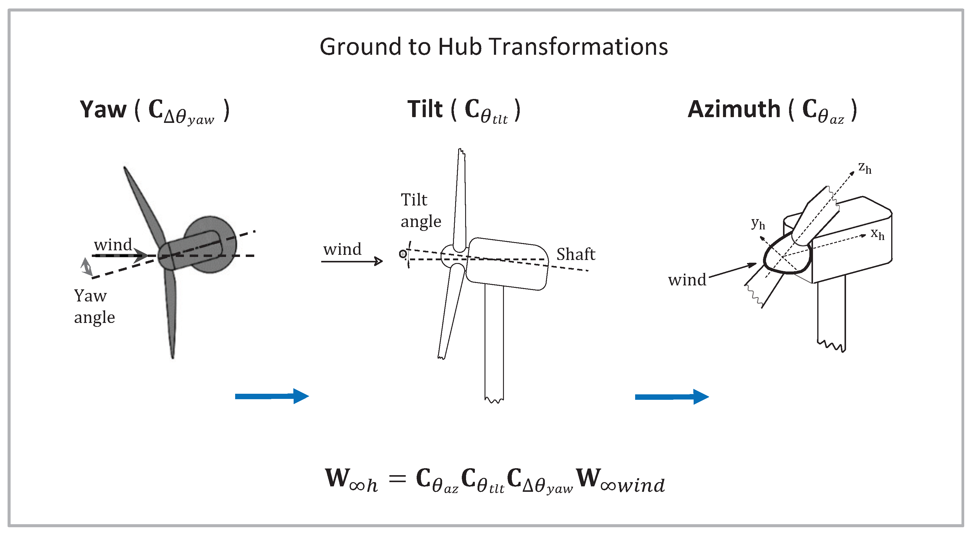
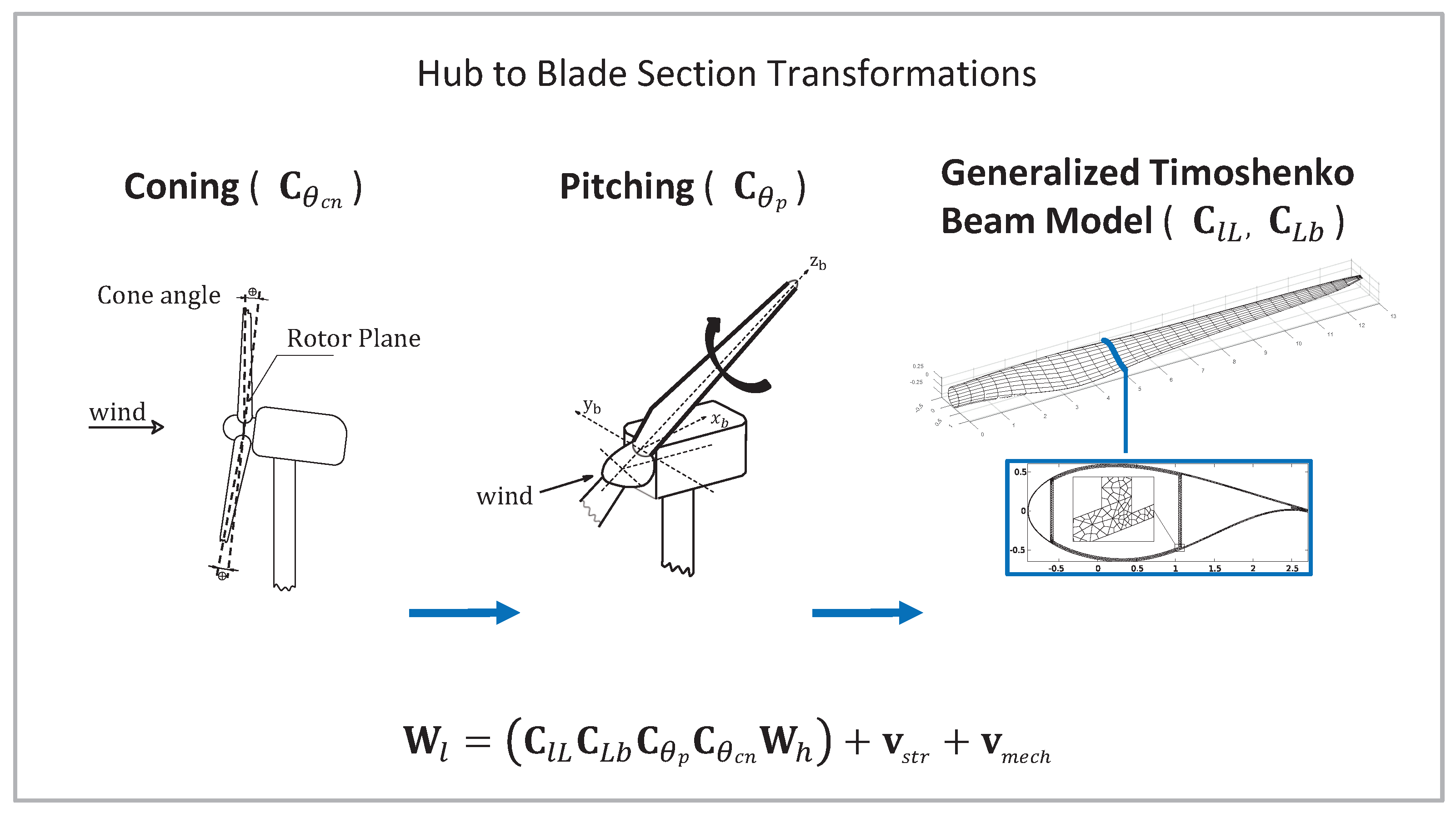
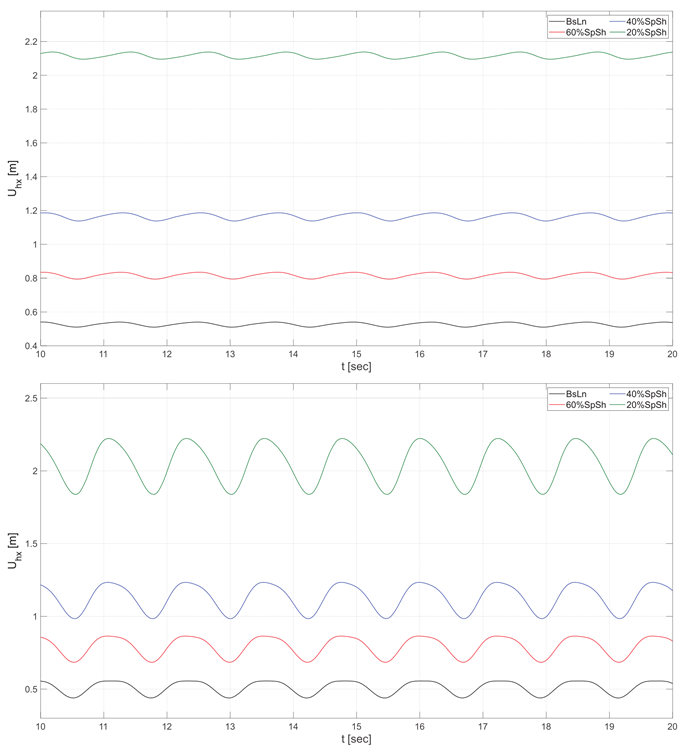
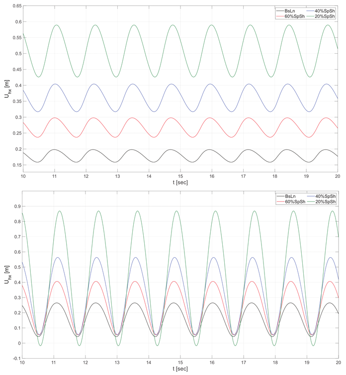
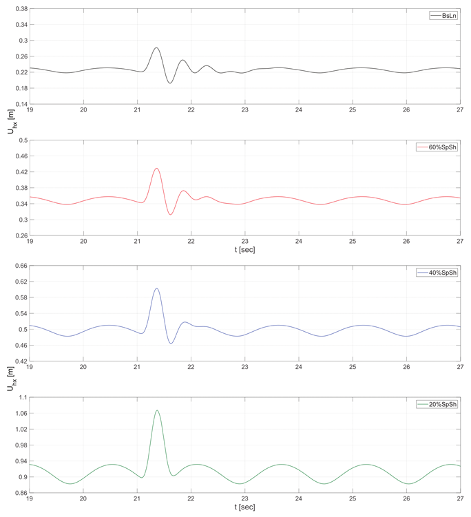
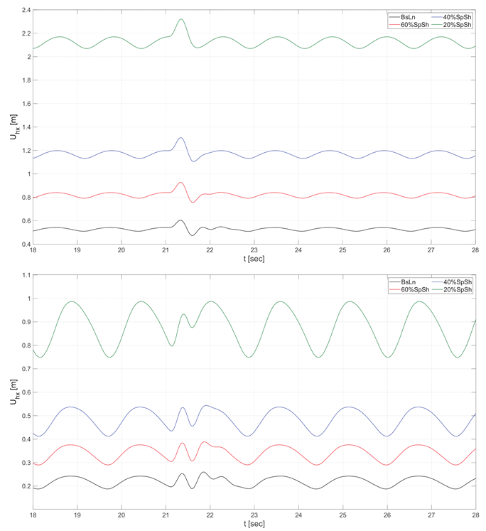
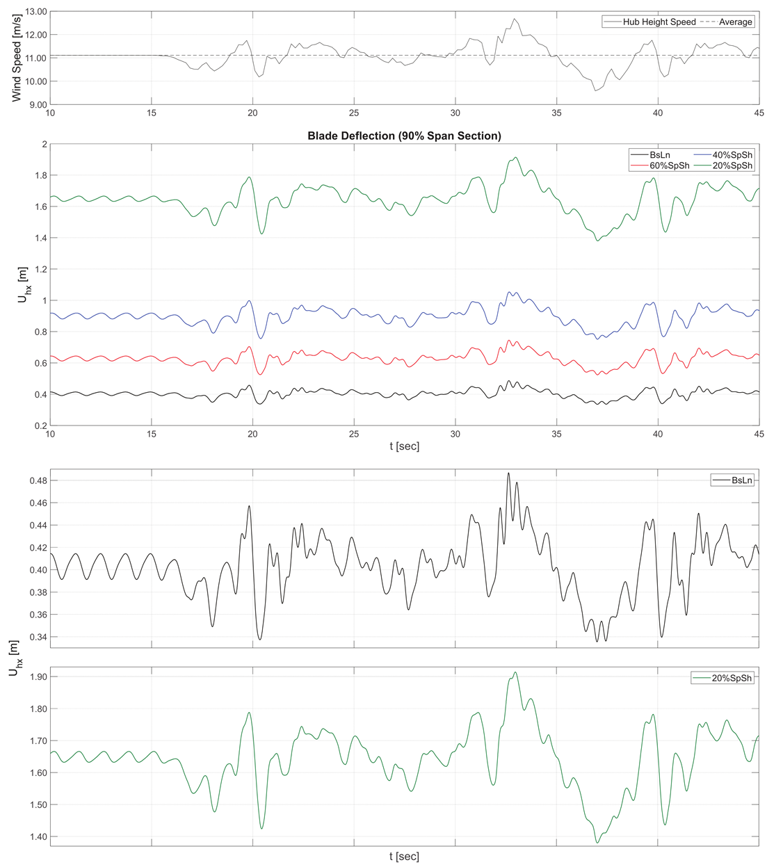
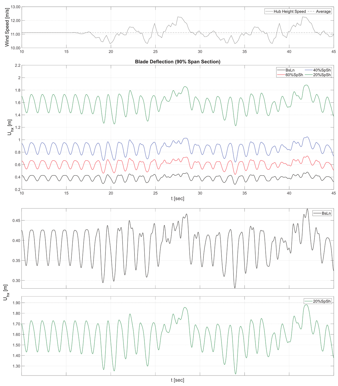
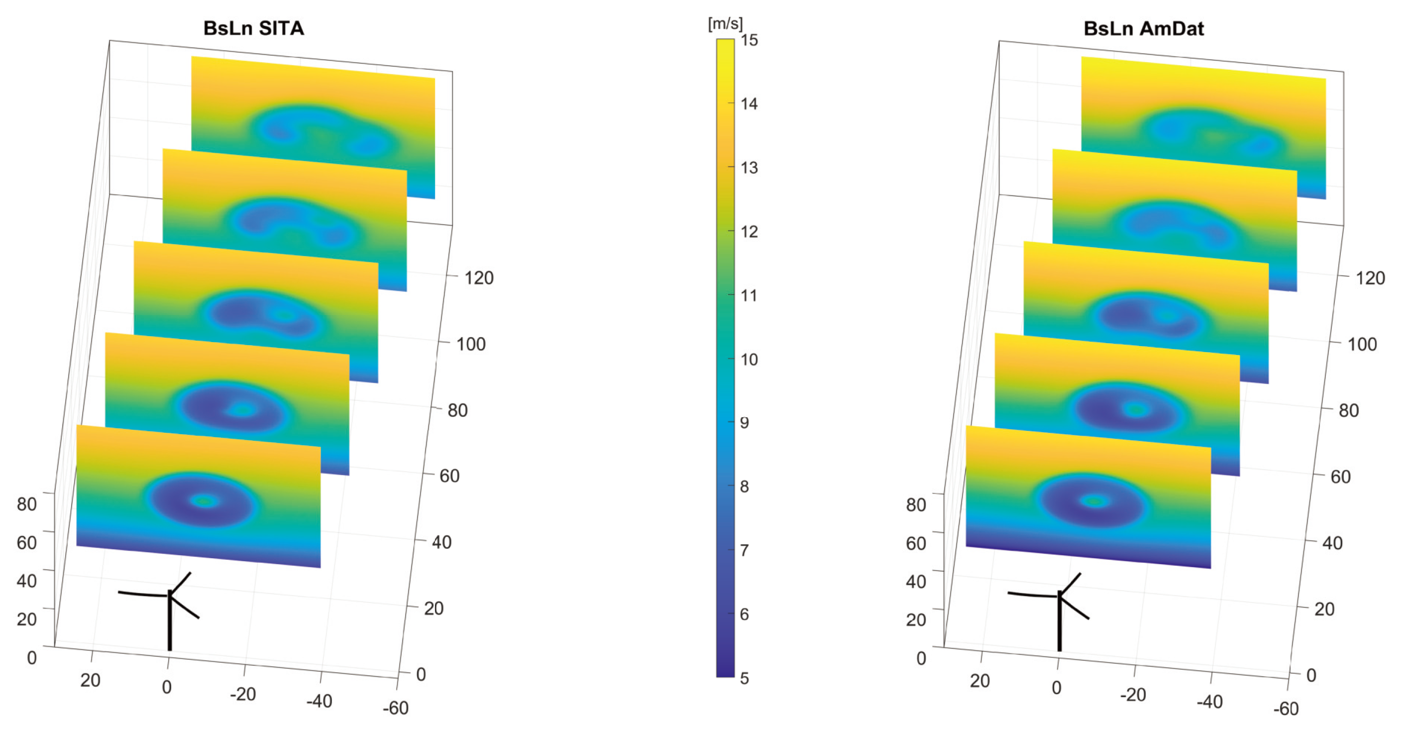
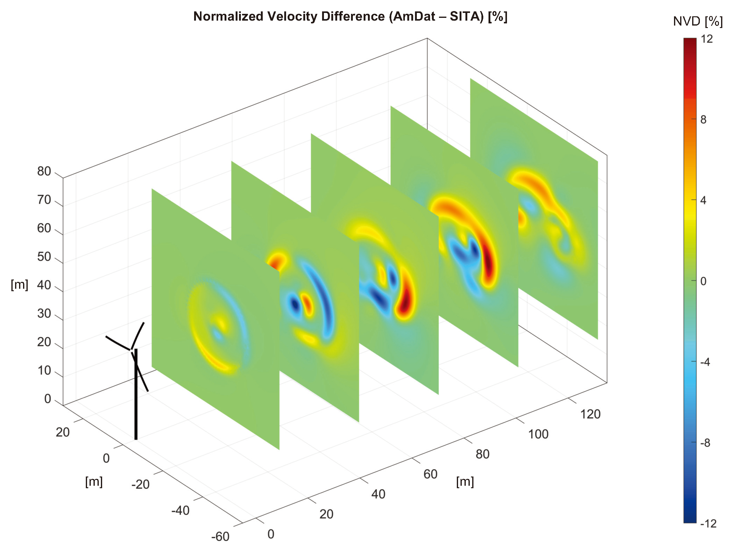