Efficient Modeling of Distributed Energy Resources’ Impact on Electric Grid Technical Losses: A Dynamic Regression Approach

Abstract

Technical losses in electrical grids are inherent inefficiencies induced by the transmission and distribution of electricity, resulting in energy losses that can reach up to 40% of the generated energy. These losses pose significant challenges to grid operators regarding energy sustainability, reliability, and economic viability. Distributed Energy Resources (DERs) offer promising solutions to lower technical losses by decentralizing energy generation and consumption, reducing the need for long-distance transmission and optimizing grid operation. Hence, estimating the impact of DERs on grid technical losses becomes paramount for grid operators and planners. In response, this article proposes the application of regression modeling and nonlinear curve fitting algorithms to provide a more nuanced understanding and better characterize the intricate interplay between DER deployment and technical losses. Through a comprehensive case study based on more than 1080 computer simulations, we demonstrate the effectiveness of our proposed dynamic polynomial varying coefficient regression model in estimating the impact of DERs on technical losses within electrical grids. The proposed model offers a simple and effective methodology that allows grid operators to gain insights into the nonlinear dynamics of DER integration and make quicker and more informed decisions regarding grid management strategies, infrastructure investments, and policy interventions. Also, this research contributes to advancing the field of grid optimization by offering a simple equation that enhances our ability and haste to assess and mitigate technical losses in the context of an evolving energy landscape characterized by increasing DER adoption.

1. Introduction

In today’s constantly changing energy landscape, integrating distributed energy resources (DERs) is gaining popularity as a vital approach to improving the power grid. These DERs, including solar photovoltaic (PV) panels, wind turbines, battery energy storage systems (BESSs), electrical vehicles (EVs), small power generators, and demand side management (DSM), have the potential to transform the conventional concept of energy generation and consumption. In recent years, DERs have emerged as critical components in transforming traditional electric grids into modern, resilient, and sustainable systems. One of the primary roles of DERs lies in enhancing grid resilience. By providing backup power during outages or natural disasters, DERs contribute to the grid’s reliability [1]. These resources can operate independently or in coordination with the main grid, mitigating disruptions and ensuring uninterrupted electricity supply to consumers. Grid stability is also bolstered by DERs, which provide ancillary services such as frequency regulation and voltage support [2]. Battery storage systems, in particular, can respond rapidly to fluctuations in supply and demand, thereby maintaining grid stability and reliability [3].

Furthermore, DERs facilitate demand response programs, allowing consumers to change their electricity usage in response to price signals or grid conditions [4]. This flexibility helps balance supply and demand, reducing the need for peaker plants and expensive infrastructure upgrades. With the rise of EVs, DERs play a pivotal role in integrating EV charging infrastructure into the grid. Smart charging stations and vehicle-to-grid (V2G) technology enable EV batteries to serve as distributed storage units, supporting grid stability and enhancing overall energy management [5]. In addition, DERs are integral to developing microgrids capable of operating equally in off-grid and on-grid modes. Microgrids enhance energy resilience by providing reliable power to critical infrastructure during emergencies or grid outages.

Last, DERs are crucial in managing peak electricity demand and alleviating grid infrastructure strain [6]. Solar panels, wind turbines, and battery storage systems can generate power during periods of high demand, reducing reliance on traditional power plants and minimizing electricity costs for consumers. Integrating renewable energy sources into the grid is another crucial function of DERs. With the increasing adoption of solar and wind energy, distributed generation technologies enable the efficient utilization of these intermittent resources. By generating electricity near where it is consumed, DERs reduce transmission losses and enhance the overall efficiency of the grid. However, integrating DERs into electrical grids presents opportunities and challenges; their full potential can only be realized if they are properly managed and optimized.

Regarding power management, DER integration has matured using advanced control techniques and accurate forecasting of renewable energy generation, load demand, and market prices. Additionally, on the energy level, DER’s contribution is well remunerated via in-place financing mechanisms such as net metering (NM), Feed-in-tariff (FiT), and power purchase agreement (PPA). Yet, other contributions, such as reducing the electric grid’s technical losses, remain less explored.

The operation of electric grids is inherently plagued by technical and nontechnical losses (

Table 1. Classification of electric grid losses.

Level 1	Level 2	Level 3	Components of Level 3
Losses	Technical Losses	Fixed Losses	Hysteresis losses Eddy current losses
		Variable Losses	Ohmic losses
	Nontechnical Losses	Network Equipment issues	Theft and fraud Measurement errors
		Network information issues	Missing or unregistered connection points Incorrect location or energization status of connection points Incorrect information on measurement equipment
		Energy data processing issues	Estimation of unmetered consumptions Estimation of consumptions between meter readings and calculations Estimation of technical losses Estimation of detected issues Other energy data processing issues

), which result in energy dissipation and reduce overall system efficiency [7]. Technical losses in the electric grid refer to the energy lost during transmission and distribution. These losses occur due to resistance in power lines, transformer inefficiencies, and voltage drops. Technical losses lead to a waste of energy and result in increased costs for energy companies and potential disruptions in electricity supply to end-users. By understanding the causes and patterns of technical losses through data analysis, energy companies can take targeted actions to reduce them. Methodologies used today to assess the technical losses rely on simulation software [8,9], measurement and verification (M&V) studies [10], load flow analysis modeling tools [11,12], and Distribution System State Estimation (DSSE) [13,14,15]. However, despite their numerous advantages, these methodologies can be computationally intensive and time-consuming and require specialized knowledge and training to be used effectively. This is where regression models come into play, offering a powerful tool to analyze historical data and identify factors that contribute to technical losses. Regression models enable energy companies to make data-driven decisions and implement strategies to improve grid efficiency.

This study introduces a dynamic polynomial regression equation with varying coefficients to evaluate the impact of Distributed Energy Resources (DERs) integration across different points of the electric grid. The equation factors in DER power, the connected load, and total impedance at the relevant bus, accurately estimating the reduction in technical losses. This dynamic regression model offers a swift and straightforward approach to assessing such reductions as an alternative to traditional methodologies. It boasts quicker results, demands less computational power, and provides comparable precision to simulation models, all without requiring specialized expertise.

This model holds promise for integration into optimization algorithms and resource allocation strategies, facilitating efficient planning while minimizing technical losses. It can also offer valuable insights into the efficacy of different control strategies. Furthermore, it can aid in the development of targeted and cost-effective control mechanisms and help identify inefficiencies within the grid.

By analyzing data on technical losses, energy companies can pinpoint specific areas or factors contributing to these losses, enabling targeted actions to enhance grid resilience, reduce costs, and improve overall operational efficiency.

In the first part of this paper, and within the literature review context, we define the technical losses and the challenges and limitations of DER penetration level in electrical grids and identify the existing methodologies and techniques used to calculate the technical losses. In the Section 3, we introduce the methodology adopted to develop, train, and test our proposed regression model, and in Section 4, we introduce the built model. Finally, in Section 5, the testing results are presented, and an analysis of the accuracy and precision of the proposed model is provided.

2. Literature Review

The integration of DER into electric grids has emerged as a critical strategy for enhancing grid resilience, sustainability, and efficiency, with publications that address their impact on the grid dating back to the 1970s. The United States Public Utility Regulatory Policies Act (PURPA) [16] encouraged the development of renewable energy and cogeneration facilities by requiring electric utilities to purchase power from qualifying facilities, which included certain types of small-scale, decentralized power generation. This provision effectively incentivized the growth of customer-owned generation, as individuals or businesses could install renewable energy systems and sell excess electricity to utilities at favorable rates.

However, the degree of integration of DERs into the electric grid, defined as the penetration level, remains controversial. A higher DER integration diversifies the energy mix and reduces dependence on fossil fuels. It also helps alleviate stress on the grid during peak periods, reducing the need for costly infrastructure upgrades. However, an excessively high level of DER penetration can pose challenges related to grid stability, voltage regulation, frequency control, and power quality, requiring advanced grid management techniques and infrastructure upgrades [17,18]. Hence, the penetration level of DERs is a key metric used to assess the impact of DERs on the grid and to gauge the extent of their integration into the overall energy system.

Various factors, including technological advancements, regulatory policies, market dynamics, and consumer preferences, influence the penetration level of DERs. The term “DER penetration level” is typically defined as the maximum power capacity of DERs relative to the total installed capacity within a given system. It measures the physical presence of DERs in terms of their maximum potential power output rather than their actual energy production. However, slight variations in how the concept is defined and used may exist in different contexts.

In contrast to capacity penetration, the DER energy penetration’s definition considers the actual energy output or contribution of DERs to the total energy consumed within a specified timeframe (e.g., hourly, daily, annually). It reflects the dynamic nature of DERs’ energy generation or consumption patterns.

Additionally, there are two other definitions: DER market penetration and DER operational penetration. The DER market penetration perspective looks at DER technologies’ market share or adoption rate within a particular market or customer segment. It considers factors such as the number of DER installations, customer participation in DER programs, and the percentage of customers with DER assets. The DER operational penetration definition focuses on the operational impact of DERs on the grid, including their influence on grid stability, reliability, and power quality. It considers factors such as DERs’ ability to provide grid support services, participate in demand response programs, and mitigate grid constraints.

By nature, DERs are located closer to demand centers, hence contributing to reducing electric grid losses by generating electricity closer to where it is consumed. This can mitigate losses incurred during long-distance transmission from centralized power plants. Electric grid technical losses, encompassing both transmission and distribution losses, represent a significant challenge in operating and managing electrical grids worldwide. These losses, arising from conductor resistance, transformer inefficiencies, and voltage drops, contribute to energy wastage, reduced system efficiency, and increased operational costs. Effective modeling of technical losses is essential for optimizing grid performance, enhancing energy efficiency, and ensuring the reliability of the electricity supply [19,20]. This literature review explores various modeling techniques employed to quantify and mitigate electric grid technical losses, encompassing both traditional and advanced approaches.

Traditional methods for modeling electric grid technical losses include empirical formulas, analytical models, and statistical regression approaches. Empirical formulas, such as the I2R formula, estimate losses based on the product of current squared and resistance. Analytical models, such as load flow analysis and network impedance methods [21,22], provide a theoretical framework for calculating losses based on grid topology and operating conditions. Statistical regression approaches, including linear and multiple linear regression, correlate technical losses with load demand, network configuration, and environmental variables. Nevertheless, recent advancements in modeling techniques have expanded the scope and accuracy of electric grid loss estimation. These techniques include machine learning algorithms, such as artificial neural networks (ANNs) [23], support vector machines (SVMs) [24], and decision trees [25]. Machine learning models offer data-driven approaches for predicting technical losses based on historical data and system parameters. These models can capture nonlinear relationships and complex interactions among variables, improving prediction accuracy. Comparably, optimization-based approaches, including genetic algorithms [26], particle swarm optimization [27], and ant colony optimization [28], optimize grid configurations and operational parameters to minimize technical losses by iteratively adjusting system parameters to achieve optimal performance while considering constraints such as voltage limits and equipment ratings. Also, several hybrid models combining multiple techniques exist [29]. A hybrid model may use machine learning for the initial prediction of technical losses and optimization algorithms for fine-tuning system parameters to minimize losses further.

Different methods are also used to allocate the losses to each load connected to the grid. The prorated methodology is a simple empirical method for the electric grid’s loss allocation (pro rata, PR). This methodology aims to equally distribute the grid losses among different components or sections of the distribution system based on their contribution to the overall energy flow, regardless of network configuration and the distance between the generator and the load [30]. The PR approach is straightforward to implement; however, it is unjust for loads located near generating sources. Hence, the distance-adjusted pro rata (DAPR) method may be a more accurate option.

The DAPR considers the distance of the load to a root node and the power demand to define the distance factors. Distance factors are calculated or assigned to each section of the distribution system based on the length of the distribution lines. Longer lines generally have higher losses due to increased resistance, so the distance factor represents the relative contribution of each section to the total line length [31]. The DAPR technique incorporates the distance factor but does not consider the nonlinearity of the power flow.

Another technique that is used is the incremental loss method. By using the linearization in the Newton–Raphson method for solving the power flow, this method calculates the incremental increase in losses caused by the addition of new components, such as transformers, conductors, or other equipment, to the existing system [32,33,34]. By quantifying these incremental losses, utilities and operators can assess the impact of new connections on system efficiency, reliability, and performance. However, high X/R ratio networks may involve complex interactions between resistive and reactive components, making the application of the incremental losses method more challenging. In contrast, network analysis approaches compute losses using the network’s impedance or admittance matrix [35]. Methods under this category include the Z-bus method [36], the modified Y-bus method [37], the branch-current decomposition method [38], and the succinct method [39].

On the other hand, the power tracing method tracks losses through branch power flow and connected nodal injections. Some existing tracing methods use graph theory, as seen in [40,41], while others utilize various algorithms [42,43,44]. Normalization is necessary if the method yields an inaccurate estimate of total losses. A comprehensive overview of loss allocation methods can be found in [45]. Additionally, for radial distribution systems with multiple distributed generation points, article [46] discusses essential considerations such as the characteristics of net generation nodes (power sources) and net load nodes (power sinks), as well as the uncertainty of distributed generator output.

By strategically locating DERs at critical points along the distribution network, utilities can optimize energy delivery, improve system efficiency, and enhance overall grid performance. Optimizing the point of integration of DERs involves selecting the most suitable location within the electrical distribution system to connect DER assets. This optimization aims to maximize the benefits of DERs while minimizing potential negative impacts on system reliability, stability, and performance. Several methods and considerations can be employed to optimize the point of connection (PoC) of DERs. Ehsan and Yang [47] provide an overview of various analytical techniques for optimal integration of DERs in power distribution systems. It reviews a range of analytical methods, including linear programming, nonlinear optimization, heuristic algorithms, metaheuristic algorithms, and artificial-intelligence-based approaches such as genetic algorithms, particle swarm optimization, and ant colony optimization.

Aryani et al. [48] explored the application of genetic algorithms (GAs) to optimize the placement and sizing of DERs in electrical distribution systems, with the main objectives of reducing power losses and improving voltage profiles within the distribution network. Avchat and Mhetre [49] optimized the placement of distributed generation (DG) within distribution networks to achieve loss reduction and voltage improvement objectives using various optimization techniques such as heuristic algorithms, mathematical programming, and evolutionary algorithms to determine the best locations for installing DG units. In the article [50], the authors explore the use of Particle Swarm Optimization (PSO) to determine DG’s optimal sizing and placement in distribution systems.

Thus, numerous case studies and applications demonstrate the effectiveness of modeling techniques for electric grid technical losses across different contexts and scales. These studies encompass urban, rural, and remote grid environments, as well as diverse energy sources and demand profiles. Researchers and practitioners have applied modeling techniques to optimize grid design, improve energy efficiency, integrate renewable energy sources, and improve grid resilience to interruptions and breakdowns. However, despite significant progress, several challenges remain in modeling electric grid technical losses. These challenges include data availability and quality, model complexity, computational requirements, and uncertainty in future scenarios (e.g., demand growth and renewable energy integration).

While simple regression models may not capture all nuances of grid losses’ estimation, their simplicity, interpretability, and efficiency make them valuable tools for initial analysis and as benchmarks for more complex models. Simple regression models often require fewer computational resources, resulting in quicker training and deployment. This can benefit tasks that demand quick predictions in real-time or near-real-time situations. Moreover, simple regression models can be easily scaled to larger data sets and applied to different regions or periods without significant adjustments. This scalability is valuable for analyzing grid losses across diverse geographic areas.

Similarly, basic regression models serve as a benchmark for assessing the effectiveness of more advanced models. By comparing the results of complex models to those of a simple regression model, analysts can assess whether the additional complexity yields significant improvements in accuracy. While dealing with limited data or noisy input variables, complex models are at risk of overfitting. Simple regression models are less susceptible to overfitting, reducing the risk of producing inaccurate estimations. Our proposed model for estimating the technical loss reduction, considering the level of DER penetration at a specific grid node as an independent variable, requires little computational power. Hence, it allows high-frequency sampling, making it perfect for calculating energy losses in real time, considering the fast-changing and intermittent nature of DERs.

Additionally, the proposed model can serve other grid management and optimization algorithms, especially in managing virtual power plants (VPPs), and financially compensates prosumers’ participation in distributed energy generation. Hence, instead of just compensating prosumers for the energy injected back into the grid, our proposed model can calculate the reduction in grid losses resulting from the prosumer’s DER connection to the grid and financially remunerate him for the saved energy. Such a model might be beneficial in increasing the viability of DER deployment in ecosystems where financial incentives, like energy rates and technology prices, are insufficient to incentivize the end users.

3. Methodology

Regression models are statistical tools that analyze the relationship between a dependent variable and one or more independent variables. In the context of energy systems, regression models can be used to predict the performance of DERs based on various factors such as weather conditions, electricity demand, and grid infrastructure.

The main idea is to develop a predictive model capable of calculating the total energy losses in a grid using a DER’s penetration level connected to a specific bus as a predictor.

The DER penetration level X is defined in the following equation:

$$X=\frac{P_{DER}}{Bus Load}\times 100$$

(1)

A significant amount of data are required to build an accurate regression model capable of estimating the impact of DER integration at any grid bus on that grid’s total losses. For this purpose, using ETAP 12.6.0 simulation software, the IEEE-33 bus grid model was used as a reference model to construct a baseline (grid details are provided in Appendix A). The baseline construction methodology was based on the following steps:

–

Simulate the baseline model without any DER integration, and calculate the total losses of the reference grid model (IEEE-33 bus)

–

Integrate a certain percentage of DER at a particular bus i, simulate the whole model, and calculate the total grid losses. The total loss output value is then logged.

–

Increase the DER penetration by a step of 5%, and repeat the simulation and calculation process. Then, this step is repeated until 100% of DER integration at bus i is achieved.

–

This process is repeated until all busses in our reference model are simulated with DER penetration levels ranging from 0% to 100% with a step of 5%.

Once the learning data are prepared, the regression model can be built. This involves training the model using historical data and optimizing its parameters to minimize the difference between the predicted and actual output. Various algorithms and techniques are available for building regression models, such as ordinary least squares, gradient descent, and machine learning algorithms like random forest and support vector regression. The choice of algorithm depends on the problem’s complexity and data availability. In our case, the least squares method was adopted to develop our regression model. This method aims to minimize the sum of the squares of the differences between the observed and predicted values, also known as residuals. So, the first step is to select a mathematical model that describes the relationship between the independent variables (predictors) and the dependent variable (outcome). For example, in simple linear regression, the model could be represented as Y = β0 + β1X + ε, where Y is the dependent variable, X is the independent variable, β0 and β1 are the coefficients, and ε is the error term. Then, we implement the independent variable data set into the regression equation to generate our predicted data set. Then, we use the gathered data in the observed data set from the constructed baseline to test the precision of the regression model by calculating the difference between the observed and predicted values for each data point. These differences are called residuals. Afterward, we adjust the model coefficients to minimize the sum of the squared residuals; hence, the term “least squares”. To assess how well the model fits the data, we examine various metrics such as the following:

–

Mean Squared Error (MSE): MSE calculates the average squared difference between predicted and actual values. It penalizes significant errors more heavily than more minor errors.

$$MSE=\frac{1}{n}{\sum }_{i=1}^n{\left({\widehat{y}}_i-{\tilde{y}}_i\right)}^2$$

(2)

where ${\widehat{y}}_i$ is the observed value, ${\tilde{y}}_i$ is the predicted value, and $n$ is the number of observations.

–

Root Mean Squared Error (RMSE): RMSE is the square root of the MSE and represents the average magnitude of the errors in the same units as the dependent variable.

–

Mean Absolute Error (MAE): MAE calculates the average absolute difference between the predicted and actual values, providing a measure of the average magnitude of the errors.

$$MAE=\frac{1}{n}{\sum }_{i=1}^n\left|{\widehat{y}}_i-{\tilde{y}}_i\right|$$

(3)

–

The coefficient of determination measures the proportion of the variance in the dependent variable explained by the model’s independent variables. It ranges from 0 to 1, where a higher value indicates a better fit of the model to the data.

$$R^2=1-\frac{{\sum }_{i=1}^n{\left({\widehat{y}}_i-{\tilde{y}}_i\right)}^2}{{\sum }_{i=1}^n{\left({\widehat{y}}_i-{\overline{y}}_i\right)}^2}$$

(4)

where ${\overline{y}}_i$ is the mean of the observed values.

–

Mean Percentage Error (MPE): MPE measures the average percentage difference between the predicted and actual values, providing insights into the average directional accuracy of the predictions.

–

Mean Absolute Percentage Error (MAPE): MAPE calculates the average percentage difference between the predicted and actual values, providing a measure of the overall accuracy of the predictions relative to the observed values.

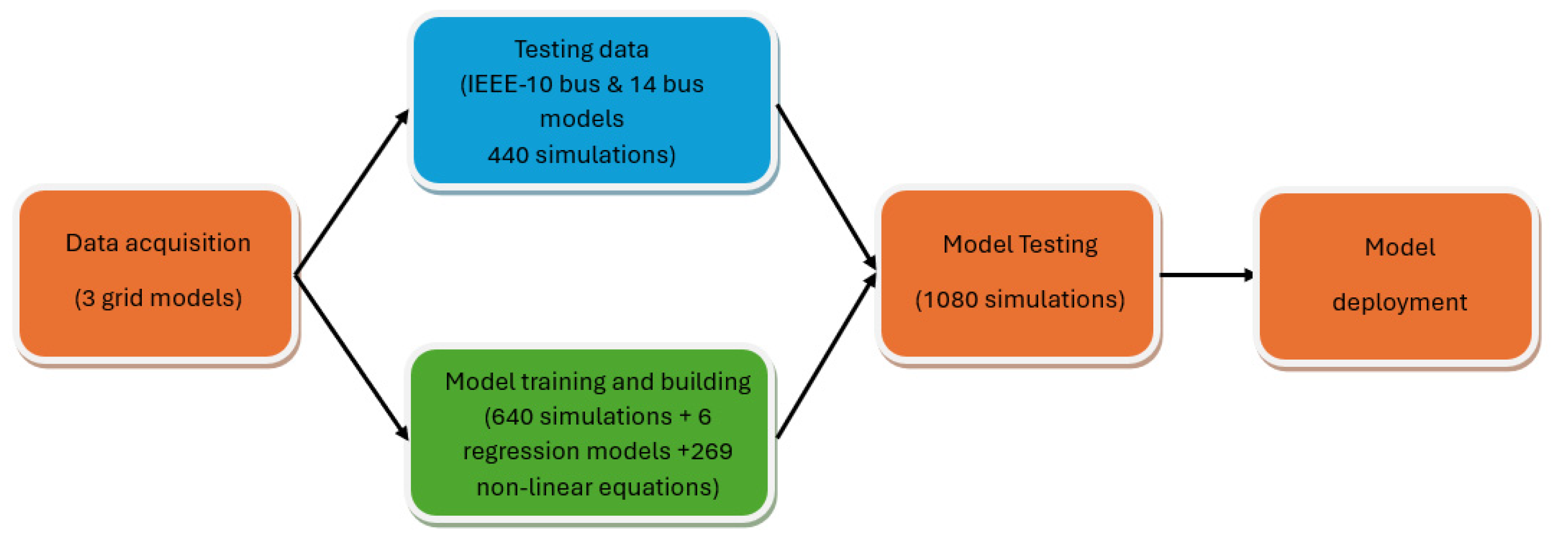
After the regression model is built, it is important to evaluate its performance to ensure its accuracy and reliability. This can be carried out by comparing the predicted values with the actual values and calculating various metrics such as mean squared error, root mean squared error, and coefficient of determination (R-squared). The performance evaluation provides insights into the effectiveness of the regression model and helps identify any areas for improvement. For this purpose, we decided to use a 14-bus grid model and the IEEE-10 bus model to test the accuracy of the proposed predictive model. Hence, 3 grid models and 1080 simulation results were used to train and test our regression model, as detailed in Figure 1.

4. Model Building

The model was built using an Intel i7-7500U, 2.70 GHz, dual-core CPU with 16 GB RAM, operating on Windows 10. The training and testing data were obtained by simulating three grid models (14-bus grid model, IEEE-10 bus, and IEEE-33 bus models) using the Electrical Transient Analyzer Program version 12.6.0 (ETAP), a software platform used to design, simulate, analyze, control, optimize, and automate electrical power systems. Both models gave practically the same results. The linear regression least square algorithm and nonlinear curve fitting algorithm were programmed using MATLAB R2022a.

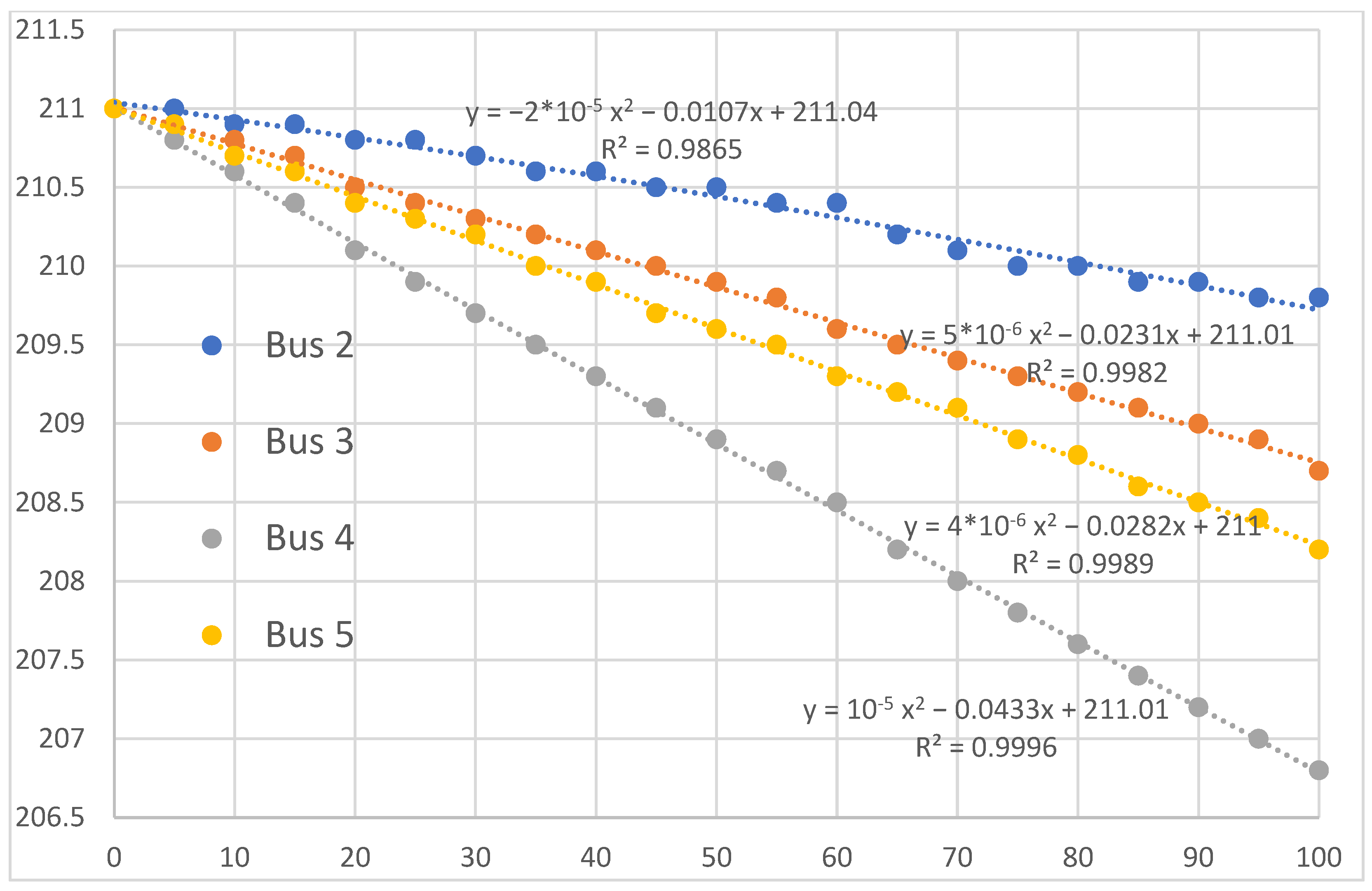
After testing various regression equations, we found that a second-degree polynomial equation best fits the data sets from different buses with an acceptable coefficient of determination (R2).

$$y=a{x}_i^2+b{x}_i+c$$

(5)

where $y$ is the estimated total technical loss in the electric grid, both variable and fixed as detailed in Table 1, and $x_i$ is the DER penetration level at bus i, as defined in Equation (1).

However, it was remarkable that the leading coefficient (a) and the linear coefficient (b) varied from bus to bus. In contrast, the constant coefficient (c) showed minor variations and could be considered constant, as illustrated in Figure 2.

Hence, we needed to identify the independent variables that affect the variabilities of coefficients a and b. It is well known that the load demand (L) directly influences active power losses in the grid. Higher loads increase line currents, leading to higher resistive losses in transmission and distribution lines. Similarly, the impedance of transmission lines contributes to resistive losses as current flows through the conductors. Higher impedance lines experience more significant losses due to increased resistance. Thus, we tried to find a relation between the coefficients a and b from one side and the total impedance Z and load L on the other.

The bus impedance $z$ (in Ohm) is calculated using the resistance $r$ and the reactance $x$ as follows:

$$z=\sqrt{x^2+r^2}$$

(6)

The total impedance $Z$ of a certain bus constitutes the sum of all the impedances from the utility grid connection to that specific bus. It is defined as the sum of the impedances of all the transmission lines and other components such as transformers, if applicable, that directly connect the power source of the grid to the subject load.

$$Z=\sum z$$

(7)

To clarify the total impedance formula, let us consider the total impedance for bus 20 of the IEEE-33 bus grid. In this case, the connection between the power source and bus 20 includes bus 0_1, bus 1_18, bus 18_19, and bus 19_20. Hence, $Z_{20}=z_1+z_{18}+z_{19}+z_{20}$.

Therefore, we moved from a simple polynomial regression model into a dynamic model with varying coefficients. A varying coefficient regression model is considered a type of dynamic regression model. Dynamic regression models are considered when the relationship between the dependent variable and the independent variables changes over time or across different subsets of the data. Varying coefficient regression models fit this definition because they allow the coefficients associated with the independent variables to vary across observations or over time.

In a varying coefficient regression model, the coefficients are not fixed but are allowed to change, which captures the dynamic nature of the relationship between the variables. This flexibility enables the model to capture complex patterns and variations in the data that traditional regression models with fixed coefficients may not adequately capture. Hence, our objective was to find functions $f_a(L,Z)$ and $f_b(L,Z)$ that define the variabilities of the leading coefficient (a) and the linear coefficient (b). So, our predictive progression model is presented by Equation (8):

$$y=f_a\left(L_i,Z_i\right).x_i^2+f_b\left(L_i,Z_i\right).x_i+c$$

(8)

The values of $a_i,b_i,c_i,L_i \mathrm{and} Z_i$ of our training model (IEEE-33 bus) are shown in

Table 2. Values of a, b, c, L, and Z of the buses in the IEEE-33 bus model.

Bus	a	b	c	Z (Ohm)	L (kW)	Bus	a	b	c	Z (Ohm)	L (kW)
2	0.000004	0.0107	211	0.4858	100	18	0.00008	0.1342	211	16.4247	90
3	0.000005	0.0231	211	1.0391	90	19	0.000009	0.0053	211	0.7125	90
4	0.00001	0.0433	211	1.4498	120	20	0.00001	0.0092	211	2.7373	90
5	0.000004	0.0282	211	1.8775	60	21	0.00001	0.0098	211	3.3670	90
6	0.000002	0.0424	211	2.9595	60	22	0.00001	0.0107	211	4.5422	90
7	0.00007	0.1513	211	3.6060	200	23	0.000008	0.0279	211	1.5856	90
8	0.0001	0.1948	211	5.7165	200	24	0.0002	0.1668	211	2.7298	420
9	0.000008	0.0639	211	6.9848	60	25	0.0003	0.1864	211	3.8675	420
10	0.00002	0.0707	211	8.2644	60	26	0.00003	0.0477	211	3.1873	60
11	0.000008	0.0548	211	8.4715	45	27	0.00004	0.0483	211	3.5063	60
12	0.00002	0.0727	211	8.8658	60	28	0.000008	0.0539	211	4.9181	60
13	0.00002	0.0793	211	10.7337	60	29	0.00005	0.1189	211	5.9847	120
14	0.00009	0.1631	211	11.6290	120	30	0.0002	0.2118	211	6.5542	200
15	0.00003	0.0835	211	12.4202	60	31	0.0001	0.1678	211	7.9054	150
16	0.00003	0.0855	211	13.3443	60	32	0.0002	0.2369	211	8.3822	210
17	0.00003	0.0863	211	15.4945	60	33	0.00003	0.0678	211	9.0126	60

.

At first, we tried to find a regression model that predicted the relation between the initial regression model’s coefficients a and b and the Load (L) and total impedance (Z). However, none of the regression models provided an acceptable coefficient of determination. Then, we decided to apply nonlinear curve fitting techniques since, as shown in Figure 3, the relation between the coefficients (a and b) and the load and impedance is nonlinear. A nonlinear curve fitting algorithm is a mathematical technique used to estimate the parameters of a nonlinear model that describes the relationship between variables in the data. Unlike linear regression, which assumes a linear relationship between the independent and dependent variables, nonlinear curve fitting algorithms allow for more complex relationships by fitting a nonlinear function to the data. These algorithms typically involve iteratively adjusting the parameters of the nonlinear model to minimize the difference between the observed and predicted values, often using optimization techniques such as gradient descent, Levenberg–Marquardt algorithm, genetic algorithms, or simulated annealing.

In our case, we used the Levenberg–Marquardt algorithm. It is an optimization technique commonly used for fitting nonlinear least squares curves. The algorithm iteratively adjusts the model’s parameters to minimize the sum of squared differences between the observed and predicted values. The Levenberg–Marquardt algorithm steps are detailed hereafter:

1. Initialization: Start with initial guesses for the model’s parameters.

2. Compute the Jacobian Matrix: Calculate the Jacobian matrix, which contains the partial derivatives of the model equations with respect to each parameter. This matrix provides information about the sensitivity of the model to changes in the parameters.

$$J_{ij}=\frac{\partial r_i}{\partial p_j}$$

(9)

where $p$ is the parameter vector, and $r$ is the residual vector.

3. Compute the Approximate Hessian Matrix: The Hessian matrix represents the second derivatives of the sum of squared residuals with respect to the parameters. In Levenberg–Marquardt, an approximate Hessian matrix is computed using the Jacobian matrix.

$$H=J^T.J$$

(10)

4. Update the Parameters: Adjust the model parameters using an iterative update rule that considers both the gradient of the objective function (sum of squared residuals) and the curvature of the objective function surface.

5. Control Step Size: The Levenberg–Marquardt algorithm uses a damping parameter, typically denoted as λ (lambda), which controls the step size during each iteration. If the step improves the fit, λ is decreased to allow larger steps. If the step worsens the fit, λ is increased to take smaller steps.

$${\lambda }_{k+1}={\lambda }_k\times \frac{trace(J^T,J)}{m\times diag(J^T.J)}$$

(11)

where

${\lambda }_k$ is the damping parameter at the k-th iteration;

$m$ is the number of observations (or residuals).

6. Convergence Criterion: Repeat steps 2–5 until a convergence criterion is met, such as reaching a specified tolerance level for the change in the parameters or the objective function.

The Levenberg–Marquardt algorithm was coded in Matlab as a function that tested 269 nonlinear equations (list of equations provided in Appendix B) to find the best nonlinear equation that defines the relation between the initial regression model’s coefficients (a) and (b) and the Load (L) and total impedance (Z). The function calculates the best curve-fitting parameters for each nonlinear equation and the Chi-square (χ²) value. The Chi-square (χ²) is a statistical measure used to evaluate the goodness of fit between observed data and expected values based on a specific model. It is commonly employed in testing the goodness-of-fit tests. The formula for the Chi-square (χ²) is given by Equation (12):

$$X^2={\sum }_i\frac{{(O_i-E_i)}^2}{E_i}$$

(12)

where

$O_i$ = Observed frequency for category $i$

$E_i$ = Expected frequency for category $i$

The complete process including the development of the linear regression models using the least square method, as well as using the Levenberg–Marquardt nonlinear curve fitting technique to define the relationship of the leading coefficient (a) and the linear coefficient (b) with respect to the Load (L) and total impedance (Z) is illustrated in Figure 4.

Using the IEEE-33 bus grid model as a learning model, we found the regression equation that allows us to calculate the total grid losses as a function of the DER level of integration at a specific grid node. The equation $y=f_a\left(L_i,Z_i\right).x_i^2+f_b\left(L_i,Z_i\right).x_i+c$, is defined as follows:

$$f_a\left(L_i,Z_i\right)=\frac{L_i}{(0.64289\times {10}^7-0.450559\times {10}^6\times Z_i)}$$

(13)

$$f_b(L_i,Z_i)=1.472\times {10}^{-4}\times Z_i\times L_i$$

(14)

$$c=Initial losses of the grid$$

(15)

If $X_i$ is defined as a percentage:

$$X=\frac{P_{DER}}{Bus Load}$$

(16)

Then, the regression model coefficients will be as follows:

$$f_a\left(L_i,Z_i\right)=\frac{L_i}{(642.896-45.0559\times Z_i)}$$

(17)

$$f_b(L_i,Z_i)=0.001472\times Z_i\times L_i$$

(18)

The precision of the developed dynamic varying coefficient was tested by comparing the predicted dependent variable outputs (generated by the regression model) to the observed dependent variable values (generated by the simulations using ETAP 12.6.0). The metrics in Section 3 were used to assess the model’s accuracy. Results are presented in

Table 3. Regression model testing results using IEEE-33 bus grid.

IEEE-33 Bus Model	MSE	RMSE	MAE	MAPE	R2
Value	3.28	1.81	1.12	0.55	0.89
Recommendation				<10	~1

.

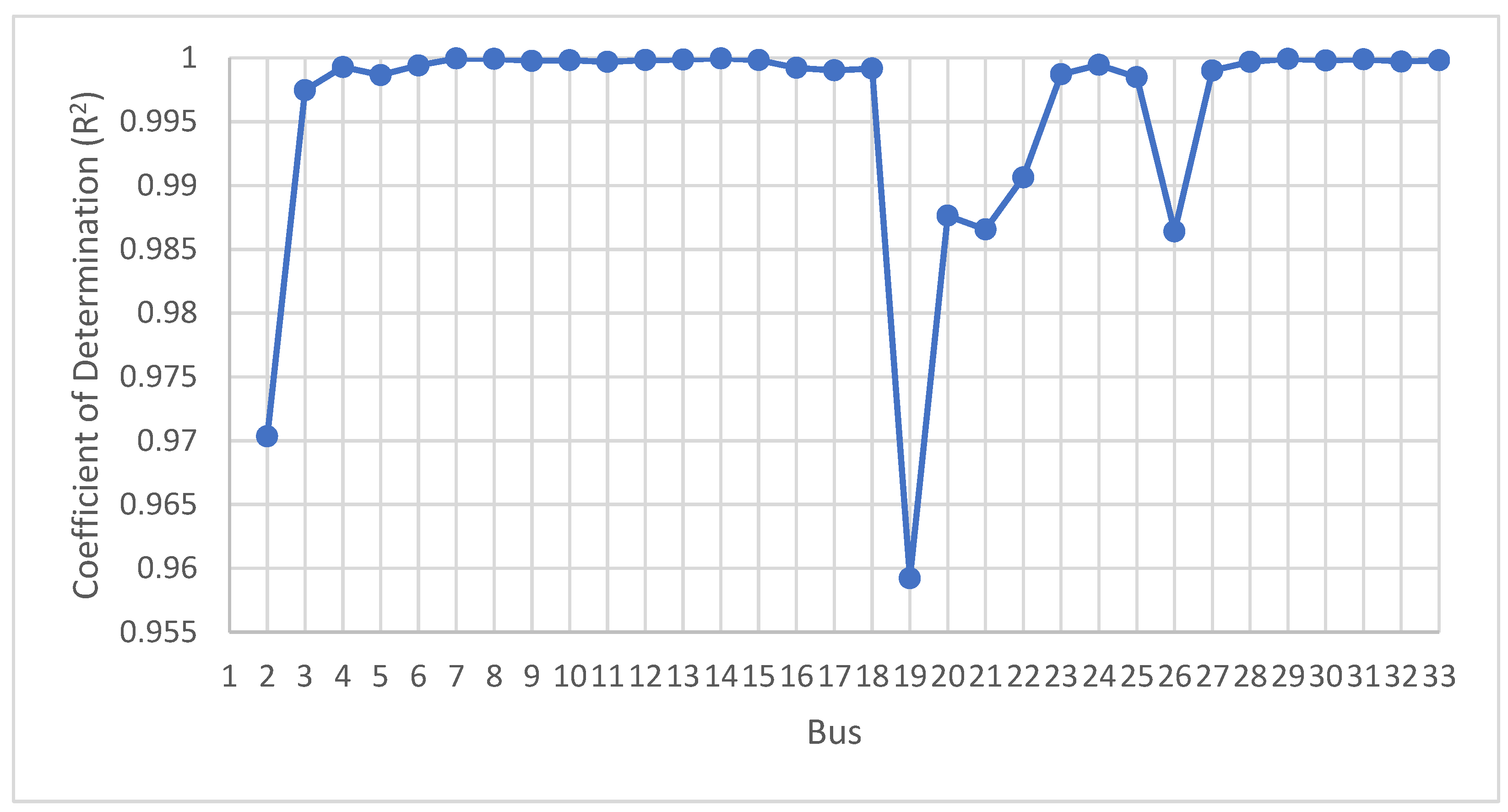
Additionally, we compared the performance of our dynamic varying coefficient regression model with a baseline model, which was, in this case, the polynomial regression model developed for each bus separately. The calculated coefficient of determinations for each bus is presented in Figure 5, while the criteria for correlation intensity in regression models according to R2 values is shown in

Table 4. Characterization of correlation intensity in regression models according to R2 values.

R2 Value	Correlation Intensity
0.00	(N) null
(0.00–0.09)	(L) low
(0.09–0.36)	(M) moderate
(0.36–0.81)	(H) high
(0.81–0.98)	(VH) very high
1.00	(P) perfect

.

To obtain a more in-depth evaluation of the performance of the proposed dynamic varying coefficient regression model, we decided to calculate the error distribution. The error distribution can help identify any systematic biases in the predictive model. The predictive model error distribution refers to the distribution of errors between the predicted values generated by the model and the actual observed values in the data set. Understanding the error distribution provides insights into the performance and reliability of the predictive model. Additionally, by analyzing the distribution of errors between predicted and actual values, you can understand the spread and variability of prediction errors, thus providing insights into how well the model captures the underlying patterns in the data. A good predictive model error distribution typically exhibits the following characteristics:

• Symmetry: The error distribution is approximately symmetric around zero, indicating that the model is equally likely to overpredict and underpredict the target variable. A symmetric error distribution suggests that the model is unbiased and does not systematically overestimate or underestimate the outcomes.
• Normality: The error distribution closely follows a normal (Gaussian) distribution. Normality implies that most prediction errors are minor, with fewer extreme errors. A normal error distribution simplifies interpretation and analysis and is often assumed by many statistical techniques.
• Constant Variance (Homoscedasticity): The variance of the errors remains relatively constant across different levels of the predictor variables. Homoscedasticity indicates that the model’s predictive performance is consistent across the entire range of the data, and the spread of errors does not systematically change with the magnitude of the predicted values.
• Zero Mean: The mean of the error distribution is close to zero, indicating that, on average, the model predictions are accurate. A non-zero mean suggests systematic bias in the model predictions, which should be investigated and corrected.
• No Outliers: The error distribution does not contain extreme outliers or anomalies. Outliers may indicate data points with unusual characteristics or errors in the data collection process. Identifying and addressing outliers is important for improving the overall reliability and performance of the model.
• Low Dispersion: The dispersion of the error distribution is relatively low, indicating that most prediction errors are concentrated around the mean. Low dispersion suggests that the model provides consistent and precise predictions with little error variability.

The error distribution of our predictive model is shown in Figure 6. The curvature of the error distribution meets the criteria of a normal error distribution curve, as detailed here.

5. Testing and Results Analysis

Following the learning phase, it is important to test the predicting model to evaluate its performance and accuracy using a separate data set not used during the training process. This process helps assess how well the model generalizes to new, unseen data and provides insights into its predictive capabilities. Hence, to obtain a separate data set that was not used during the regression model training, we used two grid models: IEEE-10 bus model and a 14-bus grid model (grid models data are provided in Appendix C and Appendix D). The testing data were generated and processed the same way as the training data, using the same simulation software, ETAP 12.6.0. Then, we used the trained regression model to predict the dependent variable using the same independent variables as the testing data set. And finally, we applied the same comparison criteria to assess the accuracy and precision of our models. Both grid model results are, respectively, shown in

Table 5. Regression model testing results using IEEE-10 bus grid.

IEEE-10 Bus Model	MSE	RMSE	MAE	MAPE	R2
Value	618.24	24.86	13.33	2.32	0.95
Recommendation				<10	~1

and

Table 6. Regression model testing results using 14-bus grid model.

14-Bus Grid Model	MSE	RMSE	MAE	MAPE	R2
Value	970.55	31.15	21.89	2.24	0.95
Recommendation				<10	~1

.

The evaluation metrics indicate that the predictive model performs well, with low error values and a high coefficient of determination (R²). Compared to a baseline model using simple polynomial regression, the developed predictive model demonstrates comparable performance, with slightly higher error metrics and lower R² value (Appendix C—

Table A5. Regression equation coefficients and coefficient of determination (CoD).

	R2	a	b	c
Bus 2	0.999773182	2.35 × 10−5	−0.06599	1116.619
Bus 3	0.999812644	1.91 × 10−5	−0.06524	1116.616
Bus 4	0.999998579	0.000353	−0.6958	1116.585
Bus 5	0.999999199	0.000479	−0.93365	1116.58
Bus 6	0.999999694	0.001858	−2.07243	1116.599
Bus 7	0.999953147	0.000752	−1.27143	1116.459
Bus 8	0.999999724	0.002145	−2.37369	1116.556
Bus 9	0.999991109	0.001346	−2.27562	1117.953
Bus 10	0.999993147	0.012075	−5.53086	1115.824
Bus 11	0.998644071	7.86 × 10−5	−0.29256	1116.588
Bus 12	0.998644071	0.001013	−0.67768	1117.429
Bus 13	0.999999455	0.002947	−2.77489	1116.533
Bus 14	0.999999423	0.002144	−2.25015	1116.548

).

While the developed predictive model demonstrates strong performance in predicting the impact of a DER integration on the total technical losses of an electric grid, several limitations should be acknowledged to provide a comprehensive understanding of its capabilities and constraints. Firstly, the model’s predictive accuracy may be influenced by the quality and representativeness of the training data. Hence, a larger data set for training might help improve the predictivity of the model.

Additionally, the analysis of the predicted values across the three tested models showed that the model tends to divert from the baseline model, thus resulting in higher error when the load connected to the bus is high and the total impedance is high. This divergence was less noticed once just one of these factors (high load or high total impedance) was applicable. Lastly, the developed dynamic varying coefficient regression model was not tested for radial topology. Additionally, the model was tested on a symmetrical balanced load, considering a pure sine wave for voltage and current. Hence, further analysis is required to test the validity of the proposed dynamic regression model for non-symmetrical unbalanced loads. Therefore, while the predictive model offers valuable insights into the impact of DER integration on the grid’s technical losses, it should be used judiciously to make informed decisions in real-world scenarios. Ongoing refinement and validation of the model are essential to address these limitations and enhance its robustness and applicability in diverse contexts.

6. Conclusions

As the energy landscape continues to evolve, optimizing DERs and minimizing technical losses in the electric grid will play an increasingly crucial role. Regression models offer a powerful tool for achieving these goals by analyzing vast amounts of data and predicting the performance of DERs. By leveraging the power of predictive modeling, grid operators, energy providers, and end consumers can unlock the true potential of DERs. This will lead to a more sustainable and efficient energy system and pave the way for a greener and more resilient future.

This article introduces a novel regression model for calculating technical losses in electric power distribution systems. Developing accurate methods for estimating technical losses is crucial for utilities to optimize their operations, enhance grid efficiency, and reduce financial losses. The regression model proposed in this study offers a data-driven approach to estimate technical losses based on key system parameters and operational characteristics such as DER integration level, line impedance, and active load connected to a certain bus. One of the strengths of the proposed dynamic varying coefficient regression model is its flexibility and simplicity, making it suitable for easy implementation in optimization algorithms, control loops, or calculation models. The main advantage of such a model is that it does not require considerable computational power or time and can be used without unique technical expertise. Moreover, we have demonstrated the model’s ability to accurately predict technical losses across various scenarios and operating conditions through comprehensive data analysis and regression modeling techniques.

While the regression model shows promising results, it is essential to acknowledge its limitations and areas for further improvement. Future research could focus on enhancing the model’s predictive capabilities by training the model with a more extensive data set and incorporating additional factors such as voltage levels, equipment conditions, and grid modernization initiatives. Furthermore, validation studies in real-world utility settings are valuable for assessing the model’s performance and practical utility.

Overall, the regression model presented in this article represents a significant advancement in technical loss calculation in electric power distribution systems as a function of the DER integration level. By providing utilities with a reliable tool for assessing the impact of DER integration level on technical losses, the model contributes to the optimization of grid operations, better selection of DER integration points for higher grid resilience and efficiency, improved energy management, and, ultimately, the delivery of reliable and cost-effective electricity to consumers. Continued research and collaboration in this area will further advance our understanding of technical losses and support the development of innovative solutions for a sustainable energy future.