1. Introduction
In Europe, traffic and transport have a major impact on air quality, especially passenger cars and commercial vehicles. The amendment to the German Climate Protection Act, which came into force on 31 August 2021, tightens the existing climate targets and stipulates the goal of greenhouse gas neutrality by 2045 [
1].
By 2030, total carbon dioxide (CO
2) emissions are to be reduced by 65% compared with the 1990 levels, and by almost 50% in the transport sector. Although CO
2 emissions from passenger cars have barely increased in recent years, according to the Transport Emission Model (TREMOD), they are still responsible for the majority of CO
2 emissions from road traffic in Germany, at over 60% [
2]. The European Green Deal has similar targets with an overall 55% reduction by 2030 [
3].
Since the vehicle emissions’ limit values for Euro 7 have recently been nearly agreed upon (see [
4]) and also since the ambitious CO
2 emissions targets for the EU’s new vehicle fleets of light-duty vehicles (LDVs) and HDVs appear to be on their way to being adopted soon, the boundaries for new vehicle technologies seem to be fixed for this decade. These regulations are expected to need high shares of electric vehicles in new registrations to meet the CO
2 fleet targets, and newly registered vehicles with combustion engines will have to meet low emission limits in most real-world driving conditions. Overall, further significant decreasing CO
2 and pollutant exhaust gas emissions from road traffic can be expected. However, the penetration of the new vehicles into the fleet needs time, and any further reductions in the emissions of the current vehicle fleet that may be necessary require traffic- and driver-related measures.
As part of the Horizon 2020 project “uCARe” [
5] (Grant agreement ID: 815002), simple and effective tools have been developed for vehicle users to reduce their individual emissions. These tools, such as a software tool to incentivize a low-emitting driving style, can have a direct impact on the overall emissions of the fleet. As a part of uCARe, a number of tools have been developed, which are used in this study.
For a holistic view of vehicle technologies and driver influences, the upstream emissions from vehicles and energy generation are also taken into account here
Especially for battery electric vehicles, the electrical energy used has GHG emissions related to production, which can vary greatly depending on the power source and, thus, contributes to national CO2 emissions.
Finally, also, so-called non-exhaust particle emissions are considered in this study. With drastically dropping tailpipe particle emissions as a result of all new cars and heavy-duty vehicles (HDVs) being equipped with particle filters, tire-, brake-, and road-wear particles are gaining increasing relevance, especially when, in the future, low PM2.5 air quality limits are to be met in the EU27 [
6].
The overall aim of this study is to assess how a vehicle user can reduce the CO2 and pollutant emissions including nitrogen oxide (NOx) and particle number (PN) by the choice of his/her vehicle and by the choice of the driving style.
2. Methods
The central point of this analysis is how the driver can influence the emissions by the choice of vehicle technology and size and by his/her driving behavior and tire selection. The effects of the avoidance of unnecessary loading, roof racks, etc., which increase tire pressure, are published in [
7].
The first aspect that the driver can influence is the vehicle technology and size. The choice of vehicle technology and size influences both CO2 emissions from vehicle production and those from vehicle operation. The following variants are compared for the vehicle technology:
The Euro 6d vehicle technology is considered representative of newly purchased vehicles. Variations of the vehicle size include the following:
The derivation of the vehicle masses for the different propulsion technologies and vehicle classes is described in
Section 2.4.
For the analysis of the impact of the driving style, three different usage profiles are compared:
The methods for modeling the eco-driver are described in
Section 2.1.2. These comparisons are made for the following trip situations:
Urban cycle to represent short-distance driving;
Average urban driving;
Average rural driving;
Average motorway driving;
A 1/3-mix of the average driving cycles to represent commuter driving.
The following sources of CO2 and pollutants are considered in this study:
Emissions from vehicles with internal combustion engines (ICEs), assuming a warmed-up exhaust gas aftertreatment (EAS) and cooling system—here referred to as “hot emissions”;
Cold start extra emissions from vehicles with ICEs;
Energy consumption of battery electric vehicles;
Additional energy consumption due to battery conditioning during the cold start of battery electric vehicles;
Particle emissions from non-exhaust sources (tire and brake wear);
CO2 emissions from fuel and electricity production on average for Europe;
CO2 emissions from vehicle production.
2.1. Simulation Tool PHEM
The “Passenger car and Heavy-duty Emission Model” (
PHEM) simulation tool has been developed by the Institute for Thermodynamics and Sustainable Propulsion Systems (ITnA) at Graz University of Technology since the late 1990s. In order to be able to take current engine and vehicle technologies into account,
PHEM is constantly being further developed.
PHEM calculates fuel consumption and exhaust emissions, as well as non-exhaust emissions (brake and tire wear) at 1 Hz for a given driving cycle. The calculation is performed based on the equations of the vehicle’s longitudinal dynamics and on engine maps for fuel consumption and emissions (
Figure 1). The engine power required for the cycles is calculated from driving resistances, the gradient, mass inertia, transmission losses, and auxiliary power consumption. The engine speed can be specified or calculated using the tire diameter and transmission ratio of the axle and the gear engaged. If the gears for a cycle are not known, the
PHEM shifting model can be used. Fuel consumption and emissions are interpolated with the engine power and speed from the maps. A routine for the simulation of the conversion efficiencies of the exhaust aftertreatment system based on the maps with the space velocity and catalyst temperature is also implemented. For selective catalytic reduction (SCR) systems, also the Ammonia (NH
3) filling level is considered. This routine calculates the component temperatures from the heat transfer between the exhaust gas and exhaust aftertreatment system, as well as between the exhaust aftertreatment system and environment. Since the vehicle’s longitudinal dynamics model calculates the engine power and speed from physical relationships, every driving condition can be represented with this model. The simulation of vehicles with different masses in combination with gradients and variable speeds and accelerations can, thus, be illustrated by the model, as well as the effects of different shifting behaviors by the driver.
PHEM can also be used to create emission maps from measured emission data. In this case, the measured emissions are gridded on emission maps according to the engine power and engine speed.
PHEM is used for many different tasks, e.g., for the simulation of emission factors for the Handbook Emission Factors for Road Transport (HBEFA) [
8,
9,
10,
11,
12].
For the simulation of hot tailpipe emissions (CO
2, NO
x, PN23, etc.), the emission maps created for HBEFA 4.1 were used. These include both the RDE and chassis dynamometer measurements of 99 diesel vehicles and 50 gasoline vehicles. These measurements were used to derive average maps based on registration statistics in order to represent the fleet mix [
13]. The BEV model is based on three measured BEVs from [
2].
The next sections show the sub-models that have been included in PHEM and deal with specific topics.
2.1.1. Cold Start Extra Emissions and Modelling
Cold Start Behavior of Combustion Engines
Cold-started internal combustion engines create a high amount of extra emissions. The cold start extra emissions (CSEEs) represent the difference in emissions between a cold-started and a hot-started cycle in g/start, as shown in
Figure 2. Most instantaneous emissions during the cold start phase are significantly higher than the emission rates under hot running conditions, as normal working temperatures (oil, cooling water, and catalytic converter temperatures) are not yet reached. Therefore, pollutants such as hydrocarbons (HCs), carbon monoxide (CO), and NO
x are not converted. Moreover, friction losses are higher in a cold engine, and combustion is impaired by a cold piston or cylinder. This leads to higher fuel consumption and, thus, higher CO
2 emissions, but also increases pollutant emissions. In
Figure 2, the influence of the cold start on the CO emissions is illustrated by the measurement of an “Inrets Urbain Fluide Court (IUFC)” cycle, which consists of a repetition of ten micro cycles. It clearly shows that, after approximately 80 s, the measured CO emissions approximate the values under hot running conditions [
14].
The CSEE level depends on vehicle-specific conditions, such as the engine type, exhaust gas aftertreatment, and corresponding pollutant class, on the start conditions, such as the ambient temperature and the parking time before the start, and on the driving style. Most pollutant emissions are higher at lower temperatures, because it takes longer for the catalytic converters to reach the required operating temperatures. Likewise, a shorter shutdown period has a positive effect on pollutant emissions, because the exhaust gas aftertreatment system does not cool down completely, so the system remains closer to the required operating temperatures. Consequently, the heat-up phase is shorter and the conversion of the pollutants starts earlier. Due to the influencing the factors mentioned above, cold start extra emissions are especially relevant in urban areas, where the cold start is responsible for more than 30% of traffic emissions [
14].
There are already some models for the representation of cold start extra emissions. One such model is “Computer Programme to calculate Emissions from Road Transport” (
COPERT version 5.7.3), a software tool coordinated by the European Environment Agency (EEA) and widely used for the mathematical modelling of air pollutant emissions from the mobile sources. In
COPERT, the additional emissions are determined as a factor of the hot emissions, considering variables such as the distance driven with a cold engine, a cold/hot emission coefficient, the average speed and temperature of the cycle, and the engine capacity. Another example is the “Methodologies for Estimating air pollutant Emissions from Transport” (MEET) method, which has a similar approach, but also includes a function to correct for very short distances [
15,
16].
Cold Start Model for Combustion Engines
The instantaneous cold start emission model suitable for implementation in the software
PHEM (version 13.0.6.13) was developed in cooperation with Eidgenössische Materialprüfungs- und Forschungsanstalt (EMPA) as a part of the H2020 project uCARe [
17]. The CSEEs (Equation (1)) are used to describe cold start emissions, since the ratio of cold/hot emissions seems to be critical for modern vehicles with very low hot emission levels. Due to the increasing relevance of cold start emissions, a development target was to design a method that can use any cold-started cycle for model parametrization. Basically, CSEEs and cold start factors need the same cycle measured once with cold and once with hot start, ideally at different start temperatures [
13]. For well-functioning modern cars, however, cold start-related emissions are much higher than hot emissions. Thus, for exhaust gas components and/or vehicles with significant cold start extra emissions, we do not need a very accurate value for the hot emission level, and we can use simulated hot emissions instead of measured ones. Inaccuracies in the simulated hot emissions do not significantly affect the accuracy for such components. For exhaust gas components with a low contribution from cold start emissions, the subtraction of the simulated hot emissions leads to a rather high uncertainty in the simulated CSEEs. However, this has little effect on the uncertainty of the total emissions (hot + cold) because of the small contribution of cold start emissions.
CSEE—Cold start extra emissions [g or #]
Ecold-measured—Measured emissions of a cycle including cold start [g or #]
Ehot-simulated—Simulated emissions of a cycle without cold start [g or #]
As the main parameter explaining the CSEEs over time, the cumulated energy loss of the combustion engine is used. This energy loss is the difference between the energy provided to the engine by the fuel and the mechanical work delivered by the engine. During the cold start, a fraction of this energy is used for heating the engine, exhaust gas aftertreatment components, and the coolant, and the rest is released via the exhaust as the enthalpy of the gas at the tailpipe. Thus, the CSEEs should depend to a large extent on this energy loss [
17].
—Energy loss of the combustion engine [kW]
—Fuel mass flow [kg/s]
—Lower heating value of the fuel [kJ/kg]
—Mechanical work delivered by the engine [kW]
—Cumulated energy loss of the combustion engine [kWh]
Also, the engine power during cold start has an impact on the emissions, resulting in increasing CSEEs for increasing power level. However, the limited number of cold start tests with different driving conditions available per vehicle does not yet allow quantifying this effect in a fleet-representative manner. The dependency of the CSEEs on
Qcum_loss is defined in the model by a polygon defining the cold start extra emissions, calculated as the measured cold start emissions minus the simulated hot emissions, over
Qcum_loss, as shown in
Figure 3. For comparability of engines of the same emissions class, but different rated power,
Qcum_loss is normalized with the rated power of the engine. For a standardized presentation, the curve consists of a number of grid points in fixed steps of
Qcum_loss [Wh/kW
nominal] [
17].
Since the temperature of the system at the time of engine start has the greatest influence on the additional cold start emissions, a relationship between Qcum_loss and the start temperature is necessary. Most of the IUFC measurements from which the CSEE curves are derived were measured between −7 °C and 20 °C ambient temperature. In order to cover a wider temperature range, measurements were also carried out with short preceding shutdown periods and, thus, higher starting temperatures. The starting temperature considered in this study is 10.5 °C and is, therefore, well covered by the measured data. For a broad applicability, however, the CSEE curve shall be mapped down to −20 °C. From the measurements, it was determined that, for the steeply rising area of the CSEE curve, there is an approximately linear relationship between Qcum_loss and the system temperature. This linear relationship was used to extrapolate the CSEE curves down to −20 °C. Both the CSEE polygons and the Qcum_loss @T-start functions are calculated by the model PHEM from the measured data specific to the exhaust component and vehicle under consideration. To simulate the CSEEs in any cycle, the model calculates the corresponding Qcum_loss @ start for a given start temperature. With this “Qcum_loss @ start” value, the CSEE polygon is entered. From this start value, Qcum_loss is increasing every second in the cycle according to the calculation of the fuel consumption and engine power in PHEM. The total CSEEs in g/start are given by the difference between the CSEE value interpolated with the resulting Qcum_loss at the end of the cold start phase and the CSEE value interpolated for Qcum_loss @ start. The instantaneous CSEEs in g/s are computed from the difference between the CSEEs in g interpolated for the Qloss per second. To simulate the start temperature for a trip with engine-off phases, a cool down curve is used, which provides the reduction of Qcum_loss as a function of the engine-off time. This enables the calculation of the starting conditions for the given engine-off duration and ambient temperature, as well as the change of Qcum_loss through engine-off phases during the cycle.
Data for calibrating NO
x, CO, HCs, and particles larger than 23 nanometers (PN23) for the emission classes Euro 3 to Euro 6d for both petrol and diesel were gathered from the European Research for Mobile Emission Sources (ERMES) [
18]. The cold start curves for diesel used in this work are based on several measurements of three vehicles each, while four vehicles were measured for the gasoline cold start curves.
For the calculation of CO2 cold start extra emissions, the method of HBEFA was applied. For this purpose, the additional CO2 emissions per start are defined for each technology, also taking into account the engine power. When calculating the individual cycles, it is first considered whether the cycle is long enough for the engine to warm up completely. If the engine does not warm up completely, only the proportional additional CO2 emissions are assigned to the cycle.
Cold Start Model for Battery Electric Vehicles
The passenger compartment and the battery have a comfortable temperature of approximately 20 °C. At lower ambient temperatures, depending on the sun radiation, heat energy is needed to meet these temperature levels. Due to the high efficiency of electric motors and the battery, only small amounts of heat are generated by losses. Thus, energy from the battery is needed for heating, whereas in vehicles with combustion engines, there is sufficient heat available due to the much lower efficiency of the engine. The energy needed for air conditioning at high ambient temperatures and sun radiation is similar to that for vehicles with combustion engines and can be considered in the simulation tool PHEM as constant additional auxiliary power, depending on the ambient conditions.
A recent study for Umweltbundesamt (UBA) Germany elaborated typical extra energy demands for the initial heating after start, as well as for the heating, ventilation, and air conditioning (HVAC) system in thermally stable conditions, i.e., after the cold start phase. The data are based on a literature review and on measurements on two battery electric vehicles (BEVs) in various real-world driving situations including low temperature tests [
2]. In addition to the basic auxiliary power consumption of approximately 300 to 600 W for the controllers, headlights, wipers, etc., the HVAC system needs between approximately 70 W (only ventilation) and up to 3000 W (heating with fresh ambient air at −20 °C).
Figure 4 shows the data used here in the simulation settings, which were calculated for Central European weather conditions (temperatures with corresponding sun radiation and humidity). As the traffic flow weighted average over all hours in a year, we calculated an approximately 550 W power demand for all auxiliaries including increased HVAC power demand due to a 10.5 °C ambient temperature.
On top of the thermally stationary power demand, the heating of the battery and the passenger compartment need heat to reach the target temperature levels after cold starts at low temperatures (“cold start extra consumption”). In [
2], 730 Wh for conditioning of the battery after a cold start at 4 °C was reported for a Volkswagen ID.3 from the measurements. The duration of the battery conditioning was approximately 15 min. From this data and the battery masses, we calculated the electric energy capacities and the specific heat capacities of the batteries as a simple equation for the cold start extra consumption (Equation (4)) for application to any BEV in simulation with the model
PHEM. The battery weight is calculated from the battery capacity using average energy densities.
—Electrical energy consumption for heating the battery cells after a cold start [Wh]
—Mass of the battery to be heated for conditioning [kg]
—Specific heat capacity of the battery [Wh/kgK]
—Temperature of the battery at start [°C]
—Target temperature of the battery for the heat-up phase, usually 15 to 20 °C
The average initial heating power for the battery is calculated using the time for the heating period, which is assumed here to be 900 s. The power for the initial heating of the passenger compartment is comparable low; see
Figure 5. After the initial heat-up time, the constantly warm air flow gradually heats up the interior.
2.1.2. Eco-Driver Model
During the H2020 project uCARe, a number of routines were developed that enable the representation of a “virtual eco-driver” [
7]. This makes it possible to simulate measured cycles both in the actual driven state and with the “virtual eco-driver”, and to assess the possible emission and energy consumption reduction rates due to an eco-driving style. These methods include the following measures:
Map-Based Gear Shifting: “Efficient Shifting”
This strategy checks all possible gears for possibly lower emission results at the same power output (including losses for shifting) compared to the pre-selected gear. The best gear that still allows the target acceleration is then selected. This shifting strategy can be applied for all exhaust components available in the engine map, as well as for a user-defined weighted mix of different pollutants [
7].
The weighting used here is carried out on the basis of the long-run climate change avoidance costs for CO
2 and on the basis of the external costs for all other pollutant components. The emission costs originate from the Handbook on the external costs of transport [
19].
Acceleration Limitation
The optimum acceleration behavior of the driver needs to find the best compromise between the lowest emissions per vehicle kilometer and the acceptance of the drivers. The first step in this analysis was to find out where the optimal speed of a vehicle is. For this purpose, a simulation of constant speed points was carried out for several vehicles.
Figure 6 shows the simulated CO
2 values of different constant speed points for the individual gears of a Euro 6d-Temp diesel vehicle. At lower speeds, the almost constant auxiliary power demand leads to high fuel consumption; at higher speeds, the air resistance increasing with the square of the speed leads to increased fuel consumption. The optimum at a constant speed, therefore, depends on the air resistance of the vehicle and the auxiliary power demand, but was always in the range of approximately 50 to 70 km/h for the vehicles considered in uCARe [
7]. It is logical that the vehicle should be operated as much as possible in the optimum speed range.
To identify the acceleration rates leading to the lowest fuel consumption per kilometer, simulations were performed in [
20]. To analyze the acceptance of the acceleration limits found in [
20], tests with four amateur drivers at the TUG were performed in [
7]. The analysis shows that driving at speeds lower than the optimum should be short, and consequently, accelerations in this speed range should be high and ideally in the area of the highest brake-specific engine efficiency. This leads to the lowest specific CO
2 emissions per km in the lower speed range. Full load should be avoided due to increasing brake-specific pollutant emissions. The acceptance of this strategy was high within the test drivers.
Above approximately 60 km/h, any acceleration increases the fuel consumption per kilometer. Accelerations in the range of the best engine efficiency at such higher speeds lead to a rapid increase in speed, which increases the driving resistance disproportionately due to the quadratic influence of the air resistance. The product of kWh/km × g/kWh is, therefore, worse than when accelerating below the point with the best engine efficiency. As a maximum speed of approximately 60 km/h was not accepted by the drivers in extra-urban trips, a gentle acceleration target was defined above the optimum speed, which drops to zero at 120 km/h. The resulting limit value for acceleration is shown as the green curve in
Figure 6. The acceleration behavior at different speeds and driving styles was validated in [
7], using 181 measurements from Heinz Steven Data Analysis and Consulting (HSDAC). The trips performed with the eco-driving style were in the area of the acceleration limit from
Figure 6, while normal and aggressive trips used much higher accelerations above the optimum speed.
The acceleration limits identified are in line with the literature data. In [
21], it was investigated how acceleration behavior can be quantified and which accelerations lead to increased fuel consumption for defined travel distances. There, an acceleration of over 0.8 m/s
2 was described as too strong. The 0.5 m/s
2 from the optimum speed selected in this study is below this limit.
The eco-driver model uses this acceleration limit in the simulation and checks every second whether the desired acceleration resulting from the measured vehicle speed trajectory is above the limit. If this is the case, the acceleration is set to the maximum allowed value at the current speed. Any resulting change in the speed curve is taken into account by a distance correction, which extends the travel time so that the same distance is covered over the entire cycle.
It should be emphasized that road safety has priority over the implementation of the driving rules. Attempts to follow them as closely as possible must not endanger other road users.
Deceleration Analysis
By limiting the maximum acceleration and maximum speed, the dynamics are limited to some extent. Besides this, the way speed reductions are realized has a high impact on energy consumption and emissions.
The idea for further investigation of the dynamics is that any energy dissipated by the mechanical brakes must be supplied again later by the engine. Exceptions to this are electric vehicles and hybrids, which can recuperate a share of brake energy, but even for these systems, avoiding unnecessary braking reduces the energy consumption and emissions due to losses in the transformation and storage of energy. The ideal deceleration is, therefore, coasting with the engine in overrun mode at low speed for a low drag torque. Since the traffic situations that would have allowed this deceleration style are not known from the recorded speed trajectory, this step is performed in post-processing based on statistical data.
The
PHEM simulation model splits the deceleration power between mechanical braking and engine braking, in addition to the deceleration caused by the driving resistances. For the post-processing model, an “eco-braking work curve” was derived from measurements with 10 test drivers by Graz University of Technology (TUG) and 181 measurements from Heinz Steven Data Analysis and Consulting (HSDAC). This shows the braking work from eco-style driven trips as a function of the average speed for flat roads. The braking work due to negative road gradients is subtracted in each trip, since mechanical braking to avoid accelerations in downhill passages cannot be avoided by eco-driving [
7].
For a simulated cycle, the average speed and the simulated average mechanical braking work are considered and compared to the equivalent value from the “eco-braking curve”, as can be seen in
Figure 7. The difference represents the statistically possible reduction in mechanical braking work. By multiplying the theoretical savings in braking energy [Wh/tkm] by the vehicle mass [t] and a vehicle-specific CO
2 factor [g/Wh], which is calculated from the trip’s average CO
2 emissions and positive engine power, we obtain the theoretical savings of CO
2 [g/km] due to reduced mechanical braking.
—CO2 savings due to reduced mechanical braking [g/km]
—Possible reduction in braking work [Wh/tkm]
—Vehicle mass [t]
—Vehicle-specific CO2 factor [g/Wh]
Figure 7.
Eco-driving mechanical braking work curve with one sample trip and braking work reduction adapted from [
7] with permission from TU Graz.
Figure 7.
Eco-driving mechanical braking work curve with one sample trip and braking work reduction adapted from [
7] with permission from TU Graz.
For the calculation of the other emission components, this factorization cannot be applied because the emission behavior is not as linearly related to the engine power as it is for CO
2. For this reason, the average emissions are divided by the average CO
2 for the total cycle. With this factor as g/gCO
2 and the CO
2 savings, the savings of the other emission components can be determined. This certainly is a drastic simplification, but no better approach to assess the savings potential due to eco-braking was identified. Since, in the post-processing of a trip, the simulation tool does not know which deceleration rates were necessary to avoid accidents, etc., the measured speed trajectory cannot be adjusted to represent eco-braking as was performed for the acceleration. Without such an adjusted speed trajectory, a detailed simulation is not possible with
PHEM. However, according to test runs with 10 different drivers in [
7,
22], the statistical approach chosen seems to give a reliable indication to the driver and what emission reductions he/she can expect by optimizing the braking behavior.
2.1.3. Non-Exhaust Particle Emission Model
Non-exhaust particle emissions (NEPs), from tire wear, brake wear, and road abrasion, have recently become more and more the focus of public attention, on the one hand, because exhaust particle emissions have become lower and lower in recent years due to increasingly restrictive emission legislation and, on the other hand, because non-exhaust emissions are rising proportionally with the increasing vehicle mileage driven. Furthermore, a limit value for brake abrasion particle emissions is already proposed for the upcoming Euro 7 legislation, which, of course, underlines the importance of investigations into non-exhaust particulate emissions [
4]. Therefore, a new simulation method for tire and brake wear was developed in the course of the H2020 uCARe project [
5]. This method was designed to allow the assessment of driving style and vehicle technology impacts on the NEPs and, thus, also uses the 1Hz driving trajectory data as the input, similar to the exhaust gas simulation. The model is implemented in the simulation tool
PHEM and is described in the following.
Simulation Approach for Brake Wear PN23 and PM
In the newly developed simulation model, the braking power and the speed of the brake disc are used as explanatory parameters for PN23 brake wear particles. The braking power is calculated in
PHEM from the equations of the longitudinal dynamics. Since the particles stored in the cavities of the pads tend to be released at higher speeds, it is assumed to have a dependence on the rotational speed of the discs. The rotational speed dependency is also shown in [
23]. In high-temperature areas of the brake pads, wear is stored also as sintered pads and resins [
24]. The formation and detachment of the pads is roughly in equilibrium, but detachment is probably more pronounced at very high temperatures and high thermal stresses. The latter effect may explain the emission peaks at the beginning of a braking process by releasing the pads formed in the previous braking event. Furthermore, at high temperatures, vaporizing binders seem to lead to a high numbers of nucleation particles. Due to a lack of test data with brake wear and temperature data, the brake temperature is not included in the model yet, although the measurements show a significant influence on the particle number emission and on the brake particle size distribution.
The brake abrasion PN23 emissions in #/s are interpolated from a characteristic curve, which is obtained from the measurement data of tests at the brake test bench. The measurement data come from the uCARe project [
5] of Worldwide Harmonized Light-Duty Vehicles Test Procedure (WLTP) brake tests and other real cycles, as well as from various brake disc and pad configurations tested in the course of the model development. The 1Hz PN23 emissions are summed up from the start of a braking process to the start of the following process and plotted over the average braking power and speed during the braking intervention. This also records the emissions that are only emitted after the brakes have been applied. For each measured brake pad and disc combination, a polygon is built from the test data (
Figure 8). In the
PHEM model, it is possible to select different PN23 characteristic curves for a single brake model or as the weighted average for the simulation. This method allows easy updates of average polygons at any time when new measurement data are available.
Figure 8 shows characteristic PN23 curves for different brake manufacturers and the average PN23 brake curve for all existing PN brake measurement data.
PM10 emissions are calculated from PN23 emissions using a density function depending on the disk speed. This reflects a trend reported, e.g., in [
23] based on systematic tests on a brake test rig, namely that the particle density [mg/#] decreases with increasing disc speed.
Simulation Approach for Tire Wear PN23 and PM
The aim in developing the model was to be able to evaluate the main influences of the driving cycle and the vehicle configuration (mass, driving resistance, etc.) on the emission values from tire wear, as already described for brake wear.
We assumed that the most important influencing factor for the mass of tire wear [mg] is the energy [kWh] transferred from the tires to the road, and therefore, the emission factors in mg/h depend on the power [kW] transferred from the wheel.
Figure 9 shows the characteristic PM10 tire wear curve (TU Graz model) implemented in the
PHEM model, as well as other representative PM10 tire wear data from the literature that are the basis of the TU Graz model curve.
PN23 is calculated via the ratio (density function) PN23/PM10. This ratio, implemented in
PHEM, is derived from the literature data [
25], as well as from test bench measurements performed at Graz University of Technology.
Figure 9.
Compilation of PM10 tire wear data (per 1 wheel) from different literature to the
PHEM model input (TU Graz Model) [
17,
26,
27,
28].
Figure 9.
Compilation of PM10 tire wear data (per 1 wheel) from different literature to the
PHEM model input (TU Graz Model) [
17,
26,
27,
28].
2.2. Validation of the Simulation Program PHEM
Validation exercises of the model
PHEM are executed regularly, to provide a statement about the model’s accuracy in the simulation of energy consumption and exhaust, as well as non-exhaust emissions. Results for diesel and petrol vehicles of different emissions standards have been published in, e.g., [
11] for HDVs and in [
9] for LDVs. For the Euro 6 passenger cars, a total of ten vehicles (five diesel and five petrol vehicles) were examined. The fuel consumption and CO
2 emissions were simulated on average in real-world driving conditions with a deviation of less than 5%. For NO
x, CO, HCs, and PM, the average deviations were below 30% and, for PN23, below 55%.
The BEV validation used measurement data for two battery electric vehicles (Volkswagen ID.3 and Renault Zoe) in several Real Driving Emissions (RDEs) runs, as well as on the chassis dynamometer. The simulation results deviated on average by 2% (Volkswagen ID.3) and 3% (Renault Zoe) from the measured energy consumption [
2].
The validation of the eco-driver model was carried out within the framework of the uCARe project and was published in [
7]. Several trips of four drivers in untrained and afterwards in instructed driving styles were examined. The trips contained a 1/3 mix of urban, rural, and motorway driving and were recorded with a portable emission measurement system. In the simulation of the untrained trips, the virtual eco-driver model showed an 11% reduction potential for CO
2. The measurement of the instructed trips showed an average reduction of 13% compared to the untrained trips. However, it should be noted that these drivers already had a normal to economical driving style.
2.3. LCA Analysis of Vehicle-, Fuel-, and Electricity-Production-Related Emissions
For a complete picture of the energy consumption and greenhouse gas emissions of different propulsion systems, a life cycle assessment (LCA) is needed, which includes emissions from fuel and electricity production, as well as vehicle production.
As part of the EU project “LONGRUN (Development of efficient and environmentally friendly LONG distance powertrain for heavy dUty trucks aNd coaches” (Grant agreement No. 874972) [
29], a tool was developed for LCA calculations of greenhouse gas emissions (gCO
2eq/km) and energy consumption (kWh/km). The tool is parameterized with an extensive collection of LCA data. The well-to-tank (WtT) GHG emissions and grey energy consumption are provided per MJ of fuel energy, while vehicle-production-related emissions are provided per mass of the main components [
30]. For this work, the forecasts for fuel and electricity production for vehicle usage for the year 2030 were used, which are based on the JRC-Eucar-Concawe collaboration (JEC) WtW report v5 [
31]. The corresponding values are shown in
Table 1.
The parameters for vehicle production were taken from a study by the Austrian Federal Environment Agency [
32], which focuses on possible vehicle production paths. The raw data for this came from the Ecoinvent database. An emission factor of 7.2 kg CO
2eq per kg vehicle weight was used for the production of vehicles with combustion engines. This value is based on the assumption that the vehicle is produced in Europe and that the electricity used corresponds to the average European electricity production mix in 2030. An emission factor of 6.2 kg CO
2eq per kg of vehicle weight was used for BEV body production without the battery, motor, and electric drive train if the vehicle production (body) is balanced with a European electricity mix. For the production of the electric engine, GHG emissions of 4.5 kg CO
2eq per kW of engine power were used. This is based on the assumption that the electric engine is produced in Europe and on the basis of the average European electricity mix. An emission factor of around 42 kg CO
2eq per kg was assumed for the production of the electric drivetrain (this includes converters, inverters, on-board charging converters, and power distributors). The literature shows GHG emissions of 61–106 kg CO
2eq per kWh of battery capacity from the production of Li-ion batteries [
33,
34,
35]. Another study [
36] forecasts an emission factor of approximately 71 kg CO
2eq per kWh of battery capacity for the production of Li-ion batteries (without climate policies) in China in 2030. This value is in the lower forecast range of previous studies and was used in our calculations. This value seems to be reasonable, as a large proportion of the vehicle batteries in use today are manufactured in China. Of course, this value can be much lower for individual companies. The total mileage over the entire life cycle of a vehicle is estimated here as 225,000 km. For BEVs, it is assumed that this mileage is achieved with a single battery [
32].
2.4. Vehicle Variations and Technologies
For the paper, virtual cars with different drive systems in identical bodies were modelled. As the basis data from Euro 6d, petrol cars for three vehicle categories—small, medium, and SUV—were used. The diesel and BEV cars for each category were derived by virtually replacing the engines and energy storage systems. This simulates the driver having identical basic vehicles just with different technologies to choose from.
Derivation of the Base Vehicle Data
The masses and rated engine power data for the base petrol vehicles were determined based on typical newly registered vehicles for the year 2022. The rolling resistance coefficient of the tires was calculated assuming a mix of three tire energy labels [
13].
Table 2 shows the tire mix and the rolling resistances for each tire label [
37]. The tire label A value was used for the simulation of the fuel-efficient tire-equipped cars.
For each vehicle technology, the same drag coefficient and cross-section air values per vehicle category were used.
Table 3 shows the main vehicle parameters.
Based on the empty weight of the base gasoline cars, the body weight for each vehicle class was calculated by subtracting the weights of the gasoline-ICE-specific components. The masses used for the components as shown in
Figure 10 were found in the literature or determined by weighing. A fuel tank capacity of 60 l was chosen, 90% filled with petrol (fuel type E5; density: 743.3 kg/m
3 for the standard condition).
The total masses for the diesel and BEV cars were calculated by adding the masses of the technology-specific components to the base petrol car body mass. The masses for the ICEs and for the electric motor depend on the rate and were calculated using the correlations specified in [
38]. The mass of the high-voltage battery for the BEVs was calculated from the battery capacity and a typical energy density. For the battery capacity, the average value for the five most registered BEVs in Austria in the year 2022 per vehicle category was used.
Table 4 shows the values for the battery capacity for the BEVs per vehicle category [
39] and the corresponding masses.
Figure 10 shows the resulting vehicle masses and the split between the main components.
The masses of the electric motors were calculated from the rated power according to [
38]. For the simulation of the exhaust emissions, the average Euro 6d maps for diesel and petrol cars were used, which were created and used for the simulation of the HBEFA 4.2 emissions factors [
13].
The characteristic curves for the battery voltage and resistance to compute charging losses and the electric motor efficiency map for the BEV were taken from data calibrated with measurements made at TUG in a project for UBA Germany [
2].
2.5. Cycles Used for Scenario Simulation
This subsection describes the cycles used for the simulation. The cycles represent average driver behavior in Germany for the following:
Urban driving;
Commuter driving;
Motorway driving.
Those cycles were derived from the HBEFA database in [
40]. A 1/3 mix of the hot emissions simulated for these three cycles in g/km represents approximately the average car usage. For adding the cold start extra emissions in g/start to the hot emissions in g/km, the cold start extra emissions are divided by the trip distance driven per cold start. Thus, cold starts have higher impacts on the results the shorter the trips are. To cover a broad range of typical mission profiles, also, a short urban trip was derived from real-world tests carried out by TUG in and around Graz, Austria.
Table 5 shows an overview of all cycles used with the most important cycle data. Also included is the 95th percentile v*apos, which represents the cycle dynamics. The higher the value, the more dynamic the cycle is. The v*apos values of the cycles used ranged from 9 to 22 m
2/s
3. The length of the individual cycles is between 3 and 260 km, the average speed between 25 and 120 km/h. If a vehicle cannot follow a speed profile because the engine is too weak or because of the eco-driver mode measures, the speed profile is automatically adjusted and the cycle is extended to cover the same distance. The simulation runs were performed individually for each combination of vehicle size and propulsion technology.
Table 5 also shows the change in average speed and 95th percentile v*apos when the cycles were simulated with the medium diesel vehicle and the eco-model.
An ambient temperature of 10.5 °C was defined for all simulations, representing the annual average for Germany in 2022 [
41].
3. Results
Calculations were performed for all combinations of vehicle category and drive technology including emissions from non-exhaust and exhaust sources including cold starts. Influences on emissions behavior from fuel-efficient tires and eco-driving are also portrayed. However, for clarity and space reasons, only selected results are compared. The results shown were always simulated with the 1/3 mix of the HBEFA average cycles. Exceptions are the cold start simulation results, where the types of cycles are listed separately.
3.1. CO2 Emissions with Effects of Vehicle Size and Driver Actions
In this comparison, the vehicle production, well-to-tank (WtT) and Tank-to-Wheel (TtW) CO
2 emissions for the vehicle sizes small, medium, and SUV were compared and the effect of eco-driving with and without fuel-efficient tires is shown and can be seen in
Figure 11. As described in
Section 2.3, CO
2eq emissions from vehicle production are attributed to a service life mileage of 225,000 km. The TtW emissions include emissions at operating temperature. The influence of the HVAC power demand at an ambient temperature of 10.5 °C was taken into account. The WtT emissions from electricity and fuel production are based on a forecast for the year 2030. The electricity used is an EU mix. With electricity from coal or purely renewable energy sources, the results are significantly different. Also, GHG emissions from battery production are related to the year 2030 in China, but can be much lower for individual companies and may further decrease in the future; see
Section 2.3.
Since only the drivetrain is exchanged in this study when comparing the drive technologies, diesel vehicles have a clear advantage over gasoline vehicles. In reality, however, diesel vehicles are, on average, heavier and more powerful than petrol vehicles, which reduces this advantage when looking at the average new vehicle fleet. The results of vehicle production, WtT, and TtW emissions of the medium vehicle are consistent with the results of current studies [
42,
43,
44]
The influence of the larger vehicle classes on the CO2 emissions is a result of the increased vehicle mass, of higher driving resistances, and of the higher rated engine power, which leads to more frequent driving in low-load areas with low fuel efficiency. The CO2 savings of diesel compared to petrol are still evident. With the electricity mix used, the electric vehicle has only approximately half the CO2 emissions of its conventional counterparts. The influence of vehicle size follows the same trend. The effect of eco-driving style and fuel-efficient tires is shown for medium cars, while the effects for small cars and SUVs follow the same trend.
For the comparison of eco-driving measures, only TtW and WtT emissions were considered. By using an eco-driving style, CO
2 emissions can be reduced by 8% (BEV), by 14% (petrol), and by 15% (diesel car). The potential savings calculated here are comparable to the results determined in [
45,
46]. A literature review in [
47] found savings potentials of 14% for eco-driving using advanced driver assistant systems in conventional cars with a standard deviation of 6%.
BEVs show less reduction potential through eco-driving measures, as most of the braking energy that is lost for vehicles with combustion engines can be recuperated. Together with the use of fuel-efficient tires, the savings potentials are 17%/20%/20%. The results from [
47] show 3–5% energy savings for the use of fuel-saving tires, but the basis for comparison (tire mix) is different here.
The CO2 emissions of the medium car types are reduced by eco-driving and the best available tire technologies to the corresponding level of the small car types with a normal driving style and average tires.
3.2. Particle Number Emissions with Effects of Vehicle Size and Driver Actions
In this comparison, the PN23 emissions from the tailpipe and non-exhaust were compared including the influence of the vehicle size and vehicle technology. In addition, the effect of eco-driving with and without fuel-efficient tires is shown for the medium car. Those results can be seen in
Figure 12.
The results of the exhaust PN23 simulation show that diesel vehicles have a clear advantage over petrol vehicles. The influence of vehicle size is also evident in the exhaust PN23 emissions of conventional vehicles, especially with petrol engines. This is due to the low rated engine power of the small vehicle, which results in higher shares of full load driving (more particles per kWh in the high-load area). These results are comparable with those from other fleet measurements. A study showed an average of 1 × 10
11 #/km for petrol vehicles in the Euro 6d emissions class in RDE measurements and an average of 3 × 10
10 #/km for diesel vehicles [
48].
In [
49], one Euro 6c petrol vehicle with GPF showed warm PN emissions of 2.9 × 10
11 #/km, which is within the spread of the Euro 6d and d-Temp cars tested for HBEFA showing a 90th percentile of 2.5 × 10
12 #/km and a 10th percentile of 2.2 × 10
9 #/km for all real-world tests.
Non-exhaust PN23 emissions increase slightly with vehicle size, and weight differences due to the engine technology within a vehicle size are also noticeable. It is noticeable that the non-exhaust particle emissions are higher than the tailpipe emissions, especially for diesel vehicles (exception: small car). Battery electric vehicles have lower emissions than their conventional counterparts, as deceleration can be largely achieved by recuperation instead of mechanical braking. However, a large part of the non-exhaust emissions comes from the tires, which are slightly higher for BEVs due to the higher vehicle mass.
Refs. [
28,
50] give on average 6 × 10
10 PN23 emissions for tire wear. Ref. [
6] reports on average 1.1 × 10
10 #/km PN23 emissions for the brake wear of vehicles. The sum corresponds with the 6.3 × 10
10 #/km PN23 emissions calculated here for the sum of tire and brake wear for the medium car.
The eco-driving behavior has a strong influence on the exhaust emissions of conventional vehicles. The exhaust PN23 emissions of the medium car can be reduced by approximately 40% (petrol) and 23% (diesel). The influence on the non-exhaust emissions of conventional vehicles is visible by a reduction of 17% (petrol) and 12% (diesel), respectively, as mechanical braking power demand can be reduced. For BEVs, the effect is only small (only 1%).
The combined use of fuel-efficient tires and the eco-driving style further increases the reduction of exhaust PN23 emissions to 47% (petrol)/28% (diesel). Although the cold start has a considerable effect on PN23 emissions, all gasoline and diesel cars are within the Not-to-Exceed limit (NTE) of 9 × 10¹¹ #/km in the urban part, as well as on the entire route.
3.3. CO2 Emissions with Effects of Cold Start and Trip Distance
This comparison shows the WtW CO
2 emissions taking into account the cold start extra emissions for the medium car such as gasoline, diesel, and BEV, and can be seen in
Figure 13. As the distance driven is essential for the cold start effect, the short city cycle (3 km), average urban cycle (19 km), average 1/3 mix, and the highway cycle were compared.
For this calculation, the ambient temperature in Germany of 10.5 °C was used [
34]. The HVAC power demand for this 10.5 °C ambient temperature and related solar radiation is included in the hot emissions. The cold start temperature used here causes significant extra emissions during initial engine heat-up for conventional vehicles, while for battery electric vehicles, it is just approximately 5 to 10 °C below the target temperature to which the battery is typically heated. This means that, at lower temperatures, the cold start effect of electric vehicles increases proportionally to the temperature difference, while conventional vehicles only emit slightly more.
Due to the significantly lower engine efficiency at low loads, conventional vehicles have higher hot emissions in the city than in the average mix. The electric vehicle has the lowest “hot” energy consumption in the city since the driving resistances are lower at lower speeds and the efficiency of the electric motor drops towards the high rotational speeds needed, e.g., in motorway driving.
The cold start effect increases the emissions of all technologies by the following values for the 3 km urban trip: 22% (BEV)/5% (petrol)/11% (diesel). Diesel vehicles have higher CO2 cold start emissions because of the higher energy demand for heating up the EAS. This is due to the lower exhaust gas temperature level and the lower heat release from HCs and CO oxidation in the catalyst compared to the petrol engines. It should be noted that the cold start is not yet completed at the end of the 3km trip for both electric and conventional vehicles. This means that a cold start effect occurs again, albeit weakened, during a subsequent ride.
If we compare the results for the urban cycle (19 km), we obtain results of a similar order of magnitude to [
51]. There, in the UDDS cycle at 20 °C, a “cold start penalty” of 6–12% is described for vehicles with ICEs and 6% for battery electric vehicles from 2013. This study also recognizes that the additional energy consumption of BEVs increases much more with decreasing temperature than for vehicles with ICEs.
For the average trip, the greatest cold start effects can be observed with electric vehicles, with the cold start increasing emissions by 3.8% (BEV)/1.0% (petrol)/2.4% (diesel) for the average trip.
3.4. NOx Emissions with Effects of Cold Start and Trip Distance
This comparison shows the NO
x emissions including the cold start extra emissions for the generic medium car, results are shown in
Figure 14. The comparison includes the same trips as used for the CO
2 comparison in
Section 3.3. The other size classes follow the same trend. The eco-driving style leads to slightly higher savings than for CO
2 (see
Figure 11), but follows a similar trend over the distance of a trip. For these two reasons, only the effect of the cold start is shown here, which is considerably higher than the driver influence.
Both diesel and petrol have the lowest hot NO
x emissions in the urban part, petrol cars being always slightly better than diesel cars (just under a factor of two). These results are comparable to those from other fleet measurements. A study showed an average of 13 mg/km for petrol vehicles in the Euro 6d pollutant class in RDE measurements and an average of 24 mg/km for diesel vehicles [
48]. Another study showed NO
x emissions of 21 mg/km for a Euro 6c petrol vehicle under hot operating conditions [
49].
The additional cold start emissions in g/start are similar for all trips; the extra emissions per km trip distance consequently are highest for the 3 km urban trip. In this situation, the tailpipe emissions per km increase by 600% (petrol)/1300% (diesel) compared to hot driving conditions. The cold start extra emissions are higher for diesel vehicles, as the heat-up of the SCR takes longer than the closed coupled three-way catalyst in petrol vehicles. The cold start effect of NO
x is completed for both technologies during this distance. For the average trip, cold start increases NO
x emissions by 34% (petrol)/100% (diesel). The additional cold start for gasoline vehicles emissions are slightly higher than stated in [
52], where approximately 200 mg/start NO
x was measured for China 6 vehicles at an average ambient temperature of 30 °C.
Although the cold start has a considerable effect on NOx emissions, both technologies are within the NTE limit of 85.5 mg/km (petrol)/114.4 mg/km (diesel) in the 19 km urban part and would also meet the limit for a 16 km trip, which is the minimum test distance for RDEs.
4. Summary and Conclusions
The work presented here intended to provide a holistic comparison of the effects of vehicle choice and driving behavior on vehicle emissions. These comparisons include the influences of the following:
Vehicle size (small car, medium car, SUV);
Vehicle technology (diesel, petrol, BEV);
Hot tailpipe emissions of CO2, NOx, and PN23 and energy consumption of BEVs;
Upstream CO2 emissions from fuel and electricity production;
Driving behavior and tire selection;
Additional emissions due to cold start effects;
PN23 emissions due to tire and brake wear.
To enable this comparison, the simulation tool PHEM was used. PHEM calculates engine, braking, and wheel power and rotational speeds from the equations of longitudinal dynamics. Based on these data, sub-models calculate the exhaust, brake, and tire wear emissions and energy consumption. The model was used to simulate generic vehicles in three size classes, namely petrol, diesel, and battery electric vehicles in different traffic situations and with different driving styles.
An increasing vehicle size proved to lead to significantly higher non-exhaust emissions and energy consumption due to the increasing vehicle mass and driving resistance. For example, WtW CO2 emissions from conventional vehicles double between small cars and SUVs, while the increase for BEVs is somewhat smaller, but also significant.
Also, the choice of vehicle technology has a significant influence on emissions. Electric vehicles, for example, have a higher mass mainly due to the battery, which means more energy is required to move them. This leads to higher tire-wear emissions, while electric braking significantly reduces brake wear particles. While electric vehicles do not generate any exhaust gases from fuel combustion, the upstream CO2 emissions from vehicle and electricity production in Europe as expected in the year 2030 correspond on average to approximately half of the CO2 emissions of ICE vehicles, including vehicle and fuel production.
The eco-driver model in PHEM enables a virtual conversion of a given driving cycle in order to assess savings potentials through driving style changes. If the production emissions are left aside, the average energy savings potential including the use of fuel-efficient tires for a conventional medium segment car is about 20%; for electric vehicles, the potential is 17%. The effect on PN23 emissions is strong for conventional vehicles, as the sum of exhaust and non-exhaust particles can be reduced by eco-driving by approximately 20% (diesel) and 35% (petrol), respectively. For battery electric vehicles, the reduction of non-exhaust particles is lower because electric braking does not produce brake wear emissions unless the maximum brake power of the motor is exceeded. Thus, look-ahead braking, which is an important element of the eco-drive style, does not influence brake abrasion greatly in normal driving situations.
For vehicles with ICEs, the cold start model calculates the additional emissions of the engine due to cold start effects as a function of the start temperature. For battery electric vehicles, the heating of the battery towards a 15° to 20 °C target temperature needs significant electric energy. For conventional cars, higher energy is needed after cold starts due to the higher friction of cold components and also due to the need for heating the exhaust aftertreatment system to reach the light-off temperatures quickly. For short distances (here, three km) with the average temperature of Germany, the cold start effect increases the CO2 emissions of conventional vehicles on average by approximately 5% to 10%, while the energy consumption of battery electric vehicles increases by more than 20%. In the average driving mix (1/3 mix), the cold start increases the consumption of conventional vehicles by approximately 1.5%, while the energy consumption of BEVs increases by approximately 4%. For NOx, the cold start effect is considerable especially for very short distances. For diesel vehicles, NOx emissions increase in the three km trip by a factor of more than 10 and, for petrol vehicles, approximately by a factor of seven, since all additional emissions are projected to a very short distance. As soon as the distance driven is increased, this effect of cold start emissions on the average g/km emissions results drops. For average driving behavior (1/3 mix), the cold start doubles the NOx emissions for diesel and increases them by 1/3 for petrol.
The non-exhaust particle emissions from tire and brake abrasion are strongly influenced by the vehicle mass, the presence of an electric motor for regenerative braking, as well as by the driving behavior. The non-exhaust PN23 emissions are approximately on the same level as the exhaust emissions. BEVs have lower non-exhaust than conventional vehicles, since recuperation during deceleration prevents brake abrasion. This outweighs the higher tire wear due to the higher vehicle mass. Hybrid vehicles, which have not been simulated in this paper, consequently, have a high reduction potential for brake wear emissions compared to the conventional ICE cars analyzed here.
Author Contributions
Conceptualization, M.O. and S.H.; methodology, M.O., S.H., C.U.M., S.L., L.L. and M.E.; software, M.O.; validation, S.H., C.U.M., L.L. and M.E.; formal analysis, M.O.; investigation, M.O., S.H., C.U.M., S.L. and L.L.; resources, M.O., S.H., C.U.M., S.L. and L.L.; data curation, M.O.; writing—original draft preparation, M.O., S.H., C.U.M., L.L. and S.L.; writing—review and editing, M.O., S.H., C.U.M., L.L. and K.W.; visualization, M.O.; supervision, M.O. and S.H.; project administration, M.O.; funding acquisition, S.H. All authors have read and agreed to the published version of the manuscript.
Funding
This research was partially funded by the European Commission in the Horizon 2020 project uCARe, Grant agreement ID: 815002 and in the Horizon 2020 project Longrun, Grant agreement ID: 874972, and from ongoing work on behalf of the HBEFA funding partners, i.e., German Environment Agency, Federal Office for the Environment FOEN, Austrian Environment Agency, Swedish Transport Administration, Norwegian Environment Agency.
Data Availability Statement
The data are contained within the article.
Acknowledgments
We would like to thank the research partners from the H2020 uCARe project, who helped us develop these models, as well as the HBEFA’s development partners, who contributed to the development.
Conflicts of Interest
Authors Silke Lipp and Konstantin Weller were employed by the company Forschungsgesellschaft für Verbrennungskraftmaschinen und Thermodynamik mbH. The remaining authors declare that the research was conducted in the absence of any commercial or financial relationships that could be construed as a potential conflict of interest.
Glossary of Terms
| approx. | approximately |
| BEV | battery electric vehicle |
| CO | carbon monoxide |
| CO2 | carbon dioxide |
| CO2eq | carbon dioxide equivalent |
| COPERT | Computer Programme to calculate Emissions from Road Transport |
| CSEE | cold start extra emissions |
| DIN | Deutsches Institut für Normung e. V. |
| DWD | Deutscher Wetterdienst |
| EAS | exhaust gas aftertreatment |
| EEA | European Environment Agency |
| EMPA | Eidgenössische Materialprüfungs- und Forschungsanstalt |
| ERMES | European Research for Mobile Emission Sources |
| EU | European Union |
| EUCAR | European Council for Automotive R&D |
| Exh. | exhaust |
| GHG | greenhouse gas |
| HBEFA | Handbook Emission Factors for Road Transport |
| HCs | hydrocarbons |
| HDV | heavy-duty vehicle |
| HSDAC | Heinz Steven Data Analysis and Consulting |
| HVAC | heating, ventilation, and air conditioning |
| ICE | internal combustion engine |
| ITnA | Institute for Thermodynamics and Sustainable Propulsion Systems |
| IUFC | Inrets Urbain Fluide Court |
| JEC | JRC-Eucar-Concawe collaboration |
| JRC | Joint Research Centre |
| LCA | life cycle assessment |
| LDV | Light-duty vehicles |
| LONGRUN | Development of efficient and environmentally friendly LONG distance poweRtrain for heavy dUty trucks aNd coaches |
| MEET | Methodologies for Estimating air pollutant Emissions from Transport |
| NEPs | non-exhaust particle emissions |
| NH3 | Ammonia |
| NOx | nitrogen oxide |
| NTE | Not-To-Exceed |
| PHEM | Passenger car and Heavy-duty Emission Model |
| PM | particle mass |
| PM10 | particle mass smaller than 10 µm |
| PN | particle number |
| PN23 | particle number with a cut-off point at 23 nm |
| PN10 | particle number with a cut-off point at 10 nm |
| Qcum_loss | cumulated heat loss |
| Qloss | heat loss |
| RDEs | Real Driving Emissions |
| RRC | rolling resistance coefficient |
| SCR | selective catalytic reduction |
| SUV | sports utility vehicle |
| T | temperature |
| TREMOD | Transport Emission Model |
| TtW | Tank-to-Wheel |
| TUG | Graz University of Technology |
| UBA | Umweltbundesamt |
| uCARe | You Can Always Reduce Emissions because you care |
| W | Watts |
| WLTP | Worldwide Harmonized Light-Duty Vehicles Test Procedure |
| WtT | well-to-tank |
| WtW | Well-to-Wheel |
References
- BGBl. I 2021 S. 3905—Erstes Gesetz zur Änderung des Bundes-Klimaschutzgesetzes. Available online: https://dejure.org/BGBl/2021/BGBl._I_S._3905 (accessed on 6 February 2024).
- Helms, H.; Bruch, B.; Räder, D.; Hausberger, S.; Lipp, S.; Matzer, C.U. Energieverbrauch von Elektroautos BEV; Graz University of Technology: Graz, Austria, 2022. [Google Scholar]
- The European Green Deal—European Commission. Available online: https://commission.europa.eu/strategy-and-policy/priorities-2019-2024/european-green-deal_en (accessed on 13 March 2024).
- European Comission. Proposal for a Regulation of the European Parliament and of the Council on Type-Approval of Motor Vehicles and Engines and of Systems, Components and Separate Technical Units Intended for Such Vehicles, with Respect to Their Emissions and Battery Durability (Euro 7) and Repealing Regulations (EC) No 715/2007 and (EC) No 595/2009; European Comission: Brussels, Belgium, 2022.
- You Can Also Reduce Emissions|uCARe Project|Results|H2020. Available online: https://cordis.europa.eu/project/id/815002/results (accessed on 6 February 2024).
- Giechaskiel, B.; Grigoratos, T.; Dilara, P.; Karageorgiou, T.; Ntziachristos, L.; Samaras, Z. Light-Duty Vehicle Brake Emission Factors. Atmosphere 2024, 15, 97. [Google Scholar] [CrossRef]
- Opetnik, M.; Hausberger, S.; Fragkiadoulakis, P.; Geivanidis, S. Software for Online and for Trip Analysis in Post-Processing with Car Owner Guidelines; European Commission: Brussels, Belgium, 2021.
- Dippold, M. PHEM—Expert User Guide for Version 13.0.6.; Graz University of Technology: Graz, Austria, 2023. [Google Scholar]
- Matzer, C.U. Bestimmung von Kraftstoffverbrauch und Abgasemissionen von Pkw in Realen Betriebszuständen Mittels Messung und Simulation. Ph.D. Thesis, Graz University of Technology, Graz, Austria, 2020. [Google Scholar]
- Zallinger, M.S. Mikroskopische Simulation Der Emissionen von Personenkraftfahrzeugen. Ph.D. Thesis, Graz University of Technology, Graz, Austria, 2010. [Google Scholar]
- Rexeis, M. Ascertainment of Real World Emissions of Heavy Duty Vehicles. Ph.D. Thesis, Graz University of Technology, Graz, Austria, 2009. [Google Scholar]
- Hausberger, S. Simulation of Real World Vehicle Exhaust Emissions; VKM-THD Mitteilungen; Verlag der Technischen Universität: Graz, Austria, 2003; ISBN 978-3-901351-74-7. [Google Scholar]
- Matzer, C.; Weller, K.; Dippold, M.; Lipp, S.; Röck, M.; Rexeis, M.; Hausberger, S. Update of Emission Factors for HBEFA Version 4.1; Final Report; Graz University of Technology: Graz, Austria, 2019. [Google Scholar]
- Hausberger, S. Umweltauswirkungen des Verkehrs: Teil Emissionen; Graz University of Technology: Graz, Austria, 2020. [Google Scholar]
- Ntziachristos, L.; Gkatzoflias, D.; Kouridis, C.; Samaras, Z. COPERT: A European Road Transport Emission Inventory Model. In Information Technologies in Environmental Engineering; Environmental Science and Engineering; Springer: Berlin/Heidelberg, Germany, 2009; pp. 491–504. ISBN 978-3-540-88350-0. [Google Scholar]
- European Comission. MEET—Methodology for Calculating Transport Emissions and Energy Consumption; European Comission: Brussels, Belgium, 1999.
- De Ruiter, J.; Indrajuana, A.; Elstgeest, M.; van Gijlswijk, R.; Ligterink, N.; Tilanus, P. Augmented Emission Maps Are an Essential New Tool to Share and Investigate Detailed Emission Data.V3; European Commission: Brussels, Belgium, 2021.
- Ermes-Group. Available online: https://ermes-group.eu/ (accessed on 13 March 2024).
- European Commission; Directorate General for Mobility and Transport; CE Delft. Handbook on the External Costs of Transport: Version 2019—1.1.; Publications Office: Luxembourg, 2020.
- Rohrmoser, T. Analytische Untersuchung der Einflüsse des Fahrstils auf Emissionen und Entwicklung Einer Bewertungsmethode; Graz University of Technology: Graz, Austria, 2021. [Google Scholar]
- Graba, M.; Bieniek, A.; Prażnowski, K.; Hennek, K.; Mamala, J.; Burdzik, R.; Śmieja, M. Analysis of Energy Efficiency and Dynamics during Car Acceleration. Eksploat. I Niezawodn.—Maint. Reliab. 2023, 25, 17. [Google Scholar] [CrossRef]
- Sarcevic, M. Optimierung des Fahrverhaltens Durch Fahrempfehlungen auf Basis von Messung und Simulation. Master’s Thesis, Graz University of Technology, Graz, Austria, 2022. [Google Scholar]
- Niemann, H. Experimentelle Einflussgrößenanalyse der Partikelemission von Pkw-Scheibenbremsen. Ph.D. Thesis, TU Darmstadt, Darmstadt, Germany, 2021. [Google Scholar]
- Breuer, B.; Bill, K.H. (Eds.) Bremsenhandbuch: Grundlagen, Komponenten, Systeme, Fahrdynamik; Springer: Wiesbaden, Germany, 2017; ISBN 978-3-658-15488-2. [Google Scholar]
- Following the Tyre Tracks… Where Do Tyre Emissions Go? Available online: https://www.emissionsanalytics.com/news/following-the-tyre-tracks-where-do-tyre-emissions-go (accessed on 6 February 2024).
- Tonegawa, Y.; Sasaki, S. Development of Tire-Wear Particle Emission Measurements for Passenger Vehicles. Emiss. Control Sci. Technol. 2021, 7, 56–62. [Google Scholar] [CrossRef]
- Environmental Protection Agency. Brake and Tire Wear Emissions from Onroad Vehicles in MOVES3; Environmental Protection Agency: Washington, DC, USA, 2020.
- Beji, A.; Deboudt, K.; Khardi, S.; Muresan, B.; Lumière, L. Determinants of Rear-of-Wheel and Tire-Road Wear Particle Emissions by Light-Duty Vehicles Using on-Road and Test Track Experiments. Atmos. Pollut. Res. 2021, 12, 278–291. [Google Scholar] [CrossRef]
- Development of Efficient and Environmental Friendly LONG Distance Powertrain for Heavy dUty Trucks aNd Coaches|LONGRUN Project|Fact Sheet|H2020. Available online: https://cordis.europa.eu/project/id/874972/de (accessed on 7 February 2024).
- Schwingshackl, M.; Rexeis, M.; Pardi, S.; El Baghdadi, M.; Gutierrez, B.A.; Hausberger, S. LONGRUN Deliverable 1.2, Integration of the LCA Analysis on the Simulation Platform with User Guide and Method Descriptions; European Commission: Brussels, Belgium, 2023. [Google Scholar]
- Prussi, M.; Yugo, M.; De Prada, L.; Padella, M.; Edwards, R. JEC Well-to-Wheels Report V5; Publications Office of the European Union: Luxembourg, 2020. [Google Scholar]
- Fritz, D.; Heinfellner, H.; Lambert, S. Die Ökobilanz von Personenkraftwagen. Bewertung Alternativer Antriebskozepte Hinsichtlich CO2-Reduktionspotential und Energieeinsparung; Vol. Reports, Band 0763; Umweltbundesamt GmbH: Wien, Austria, 2021; ISBN 978-3-99004-586-2. [Google Scholar]
- Emilsson, E.; Dahllöf, L. Lithium-Ion Vehicle Battery Production Status 2019 on Energy Use, CO2 Emissions, Use of Metals, Products Environmental Footprint, and Recycling; IVL Swedish Environmental Research Institute: Stockholm, Sweden, 2019. [Google Scholar] [CrossRef]
- Helms, H.; Biemann, K.; Lambrecht, U.; Jöhrens, J.; Meyer, K. Klimabilanz von Elektroautos: Einflussfaktoren und Verbesserungspotential; 2019; Available online: https://trid.trb.org/View/1637972 (accessed on 4 April 2024).
- Melin, H.E. Analysis of the Climate Impact of Lithium-Ion Batteries and How to Measure It; Circular Energy Storage-Research and Consulting: London, UK, 2019; pp. 1–17. [Google Scholar]
- Xu, C.; Steubing, B.; Hu, M.; Harpprecht, C.; Van Der Meide, M.; Tukker, A. Future Greenhouse Gas Emissions of Automotive Lithium-Ion Battery Cell Production. Resour. Conserv. Recycl. 2022, 187, 106606. [Google Scholar] [CrossRef]
- European Comission. Regulation—1222/2009; European Comission: Brussels, Belgium, 2009.
- Beermann, M.; Canella, L.; Jungmeier, G.; Pucker, J.; Hausberger, S.; Lipp, S. Lebenszyklusanalyse zur Gesamtheitlichen Ermittlung der Treibhausgas-Emissionen und Es Primärenergie-Verbrauchs von Transportsystemen; Verlag der Technischen Universität Wien: Vienna, Austria, 2018. [Google Scholar]
- Bundesamt für Statistik (Schweiz) Anzahl der Neuzulassungen von Elektroautos in Österreich nach Modell in den Jahren 2022 und 2023. Available online: https://de.statista.com/statistik/daten/studie/575997/umfrage/meistverkaufte-elektrofahrzeuge-in-oesterreich-nach-modell/ (accessed on 6 February 2024).
- Politschnig, N. Analyse des Realen Emissionsverhaltens von Euro 6 Diesel—Personenkraftwagen. Master’s Thesis, Graz University of Technology, Graz, Austria, 2019. [Google Scholar]
- DWD Entwicklung der Jahresmitteltemperatur in Deutschland in Ausgewählten Jahren von 1960 Bis 2023. Available online: https://de.statista.com/statistik/daten/studie/914891/umfrage/durchschnittstemperatur-in-deutschland/ (accessed on 6 February 2024).
- Pero, F.D.; Delogu, M.; Pierini, M. Life Cycle Assessment in the Automotive Sector: A Comparative Case Study of Internal Combustion Engine (ICE) and Electric Car. Procedia Struct. Integr. 2018, 12, 521–537. [Google Scholar] [CrossRef]
- Held, M.; Schücking, M. Utilization Effects on Battery Electric Vehicle Life-Cycle Assessment: A Case-Driven Analysis of Two Commercial Mobility Applications. Transp. Res. Part D Transp. Environ. 2019, 75, 87–105. [Google Scholar] [CrossRef]
- Mayyas, A.; Omar, M.; Hayajneh, M.; Mayyas, A.R. Vehicle’s Lightweight Design vs. Electrification from Life Cycle Assessment Perspective. J. Clean. Prod. 2017, 167, 687–701. [Google Scholar] [CrossRef]
- Barth, M.; Boriboonsomsin, K. Energy and Emissions Impacts of a Freeway-Based Dynamic Eco-Driving System. Transp. Res. Part D Transp. Environ. 2009, 14, 400–410. [Google Scholar] [CrossRef]
- Kato, H.; Ando, R.; Kondo, Y.; Suzuki, T.; Matsuhashi, K.; Kobayashi, S. Comparative Measurements of the Eco-Driving Effect between Electric and Internal Combustion Engine Vehicles. In Proceedings of the 2013 World Electric Vehicle Symposium and Exhibition (EVS27), Barcelona, Spain, 17–20 November 2013; IEEE: Piscataway, NJ, USA, 2013; pp. 1–5. [Google Scholar]
- Fontaras, G.; Zacharof, N.-G.; Ciuffo, B. Fuel Consumption and CO2 Emissions from Passenger Cars in Europe—Laboratory versus Real-World Emissions. Prog. Energy Combust. Sci. 2017, 60, 97–131. [Google Scholar] [CrossRef]
- Valverde Morales, V. Exhaust Emissions of In-Use Euro 6d-TEMP and Euro 6d Vehicles in WLTP and RDE Conditions, a Comparison. SAE Int. J. Adv. Curr. Pract. Mobil. 2022, 5, 1230–1242. [Google Scholar] [CrossRef]
- Pielecha, J.; Merkisz, J. Selection of a Particulate Filter for a Gasoline-Powered Vehicle Engine in Static and Dynamic Conditions. Energies 2023, 16, 7777. [Google Scholar] [CrossRef]
- Gaining Traction, Losing Tread Pollution from Tire Wear Now 1,850 Times Worse than Exhaust Emissions. Available online: https://www.emissionsanalytics.com/news/gaining-traction-losing-tread (accessed on 14 March 2024).
- Lohse-Busch, H.; Duoba, M.; Rask, E.; Stutenberg, K.; Gowri, V.; Slezak, L.; Anderson, D. Ambient Temperature (20°F, 72°F and 95°F) Impact on Fuel and Energy Consumption for Several Conventional Vehicles, Hybrid and Plug-In Hybrid Electric Vehicles and Battery Electric Vehicle. In Proceedings of the SAE 2013 World Congress & Exhibition, Detroit, MI, USA, 8 April 2013; p. 2013-01–1462. [Google Scholar]
- He, L.; You, Y.; Zheng, X.; Zhang, S.; Li, Z.; Zhang, Z.; Wu, Y.; Hao, J. The Impacts from Cold Start and Road Grade on Real-World Emissions and Fuel Consumption of Gasoline, Diesel and Hybrid-Electric Light-Duty Passenger Vehicles. Sci. Total Environ. 2022, 851, 158045. [Google Scholar] [CrossRef] [PubMed]
Figure 1.
Schematic illustration of the
PHEM simulation tool [
8].
Figure 1.
Schematic illustration of the
PHEM simulation tool [
8].
Figure 2.
CO emissions of a Euro 6d petrol vehicle in an IUFC cycle at a 20 °C ambient temperature.
Figure 2.
CO emissions of a Euro 6d petrol vehicle in an IUFC cycle at a 20 °C ambient temperature.
Figure 3.
Schematic picture of a polygon for the cumulated CO cold start extra emissions over Qcum_loss with the routine for calculating CSEEs from the polygon.
Figure 3.
Schematic picture of a polygon for the cumulated CO cold start extra emissions over Qcum_loss with the routine for calculating CSEEs from the polygon.
Figure 4.
Average power consumption of the auxiliaries of BEVs after the cold start phase as a function of ambient temperature based on [
2].
Figure 4.
Average power consumption of the auxiliaries of BEVs after the cold start phase as a function of ambient temperature based on [
2].
Figure 5.
Energy demand for initial heat-up of the battery and passenger compartment of a BEV car, calculated for a 55 kWh battery capacity.
Figure 5.
Energy demand for initial heat-up of the battery and passenger compartment of a BEV car, calculated for a 55 kWh battery capacity.
Figure 6.
Acceleration limit used in this study for eco-driving based on an analysis of the optimum vehicle speed.
Figure 6.
Acceleration limit used in this study for eco-driving based on an analysis of the optimum vehicle speed.
Figure 8.
Characteristic PN23 brake wear curves for different brake manufacturers.
Figure 8.
Characteristic PN23 brake wear curves for different brake manufacturers.
Figure 10.
Vehicle masses for the generic gasoline, diesel, and BEV cars used in the paper.
Figure 10.
Vehicle masses for the generic gasoline, diesel, and BEV cars used in the paper.
Figure 11.
CO2 emissions with the effects of vehicle size and driver actions including vehicle production (“petrol production”, “diesel production”, “BEV production”), well-to-tank, and Tank-to-Wheel emissions.
Figure 11.
CO2 emissions with the effects of vehicle size and driver actions including vehicle production (“petrol production”, “diesel production”, “BEV production”), well-to-tank, and Tank-to-Wheel emissions.
Figure 12.
PN23 emissions from exhaust including cold start and non-exhaust with effects of vehicle size and driving style including usage of eco-tires.
Figure 12.
PN23 emissions from exhaust including cold start and non-exhaust with effects of vehicle size and driving style including usage of eco-tires.
Figure 13.
CO2 emissions with effects of trip distance including cold start and hot emissions considering Well-to-Wheel emissions.
Figure 13.
CO2 emissions with effects of trip distance including cold start and hot emissions considering Well-to-Wheel emissions.
Figure 14.
NOx emissions with effects of trip distance including cold start and hot emissions.
Figure 14.
NOx emissions with effects of trip distance including cold start and hot emissions.
Table 1.
Well-to-tank data used for LCA calculation with estimations for 2030 [
31].
Table 1.
Well-to-tank data used for LCA calculation with estimations for 2030 [
31].
| Fuel Type | WtT GHG Emissions [gCO2eq/MJ] | WtT Grey Energy Demand [MJ/MJ] |
|---|
| Diesel blend | 21.3 | 0.33 |
| Gasoline blend | 17.9 | 0.31 |
| EU grid average | 74.5 | 1.34 |
Table 2.
Mix of tire labels used for all simulated cars.
Table 2.
Mix of tire labels used for all simulated cars.
| Tire Label | RRC [kg/t] | Share [%] |
|---|
| E | 9.44 | 20 |
| C | 8.12 | 50 |
| B | 6.89 | 30 |
| A: fuel efficient tires | 5.76 | |
Table 3.
Base vehicle data.
Table 3.
Base vehicle data.
| Parameter | Small Car | Medium Car | SUV |
|---|
| Rated power in kW | 55 | 110 | 160 |
| Cd × A in m2 | 0.647 | 0.652 | 0.780 |
| RRC in kg/ton | 8.02 | 8.02 | 8.02 |
| DIN empty weight of the base petrol car in kg | 974 | 1147 | 1415 |
Table 4.
Battery capacity used for the BEVs per vehicle category.
Table 4.
Battery capacity used for the BEVs per vehicle category.
| Parameter | Small Car | Medium Car | SUV |
|---|
| Battery capacity in kWh | 41 | 61 | 79 |
| Battery mass in kg | 255 | 384 | 496 |
Table 5.
Characteristics of the cycles used for the simulation including changes to the eco-driving style.
Table 5.
Characteristics of the cycles used for the simulation including changes to the eco-driving style.
| Cycle | Short-Distance
Urban Cycle | Avg. Urban Cycle | Avg. Rural Cycle | Avg. Motorway Cycle |
|---|
| Duration [s] | 400 | 2814 | 4947 | 7877 |
| Length [km] | 3 | 19 | 94 | 260 |
| Avg. v [km/h] | 25 | 25 | 68 | 119 |
| Max. v [km/h] | 47 | 81 | 92 | 167 |
| Gradient included | Yes | No | No | No |
| 95% perc. V*apos [m2/s2] | 9.1 | 13.9 | 16.4 | 21.3 |
| Duration when eco-driven [s] 1 | 400 | 2827 | 5012 | 8584 |
| Avg. v when eco-driven [km/h] 1 | 25 | 25 | 68 | 109 |
| 95th perc. v*apos when eco-driven [m2/s2] 1 | 9.1 | 11.8 | 10.7 | 8.8 |
| Disclaimer/Publisher’s Note: The statements, opinions and data contained in all publications are solely those of the individual author(s) and contributor(s) and not of MDPI and/or the editor(s). MDPI and/or the editor(s) disclaim responsibility for any injury to people or property resulting from any ideas, methods, instructions or products referred to in the content. |
© 2024 by the authors. Licensee MDPI, Basel, Switzerland. This article is an open access article distributed under the terms and conditions of the Creative Commons Attribution (CC BY) license (https://creativecommons.org/licenses/by/4.0/).


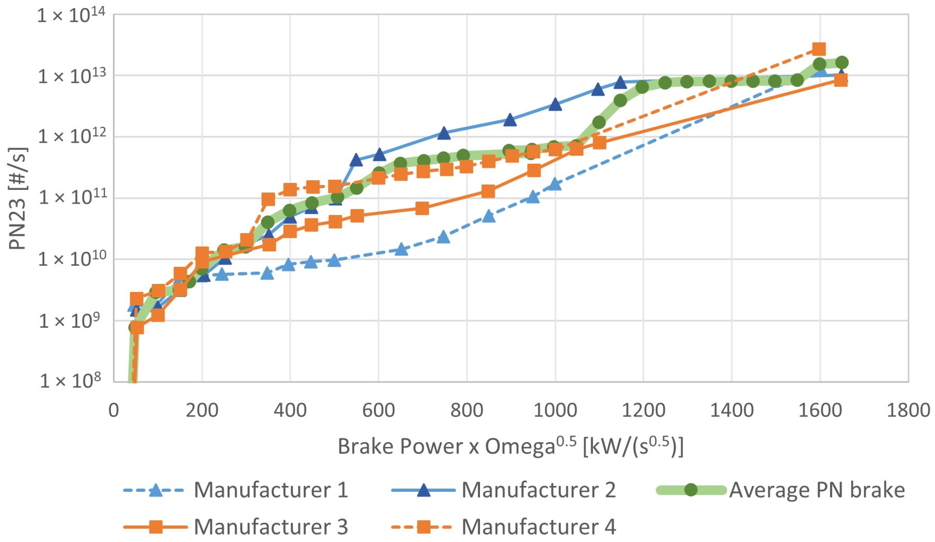
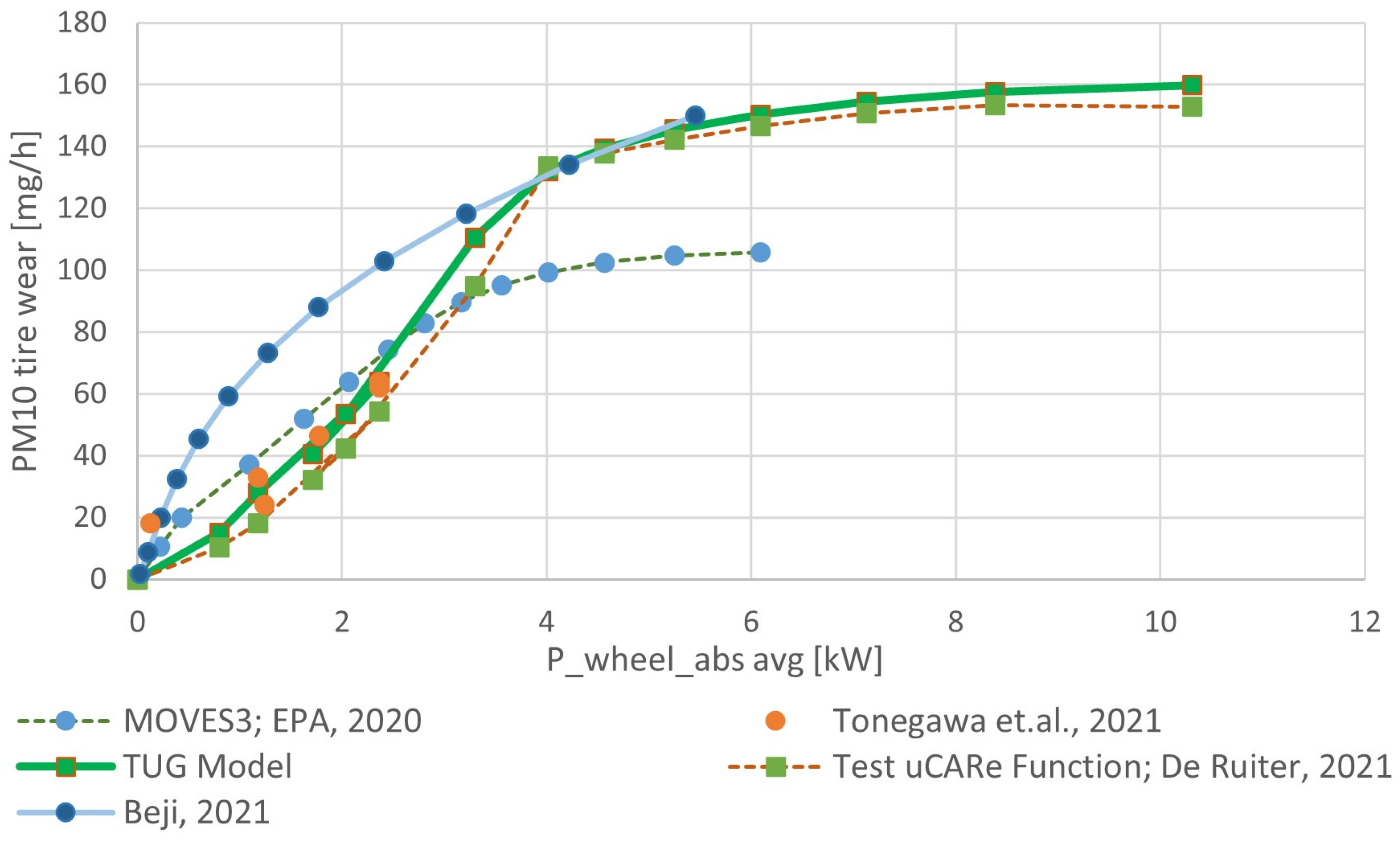
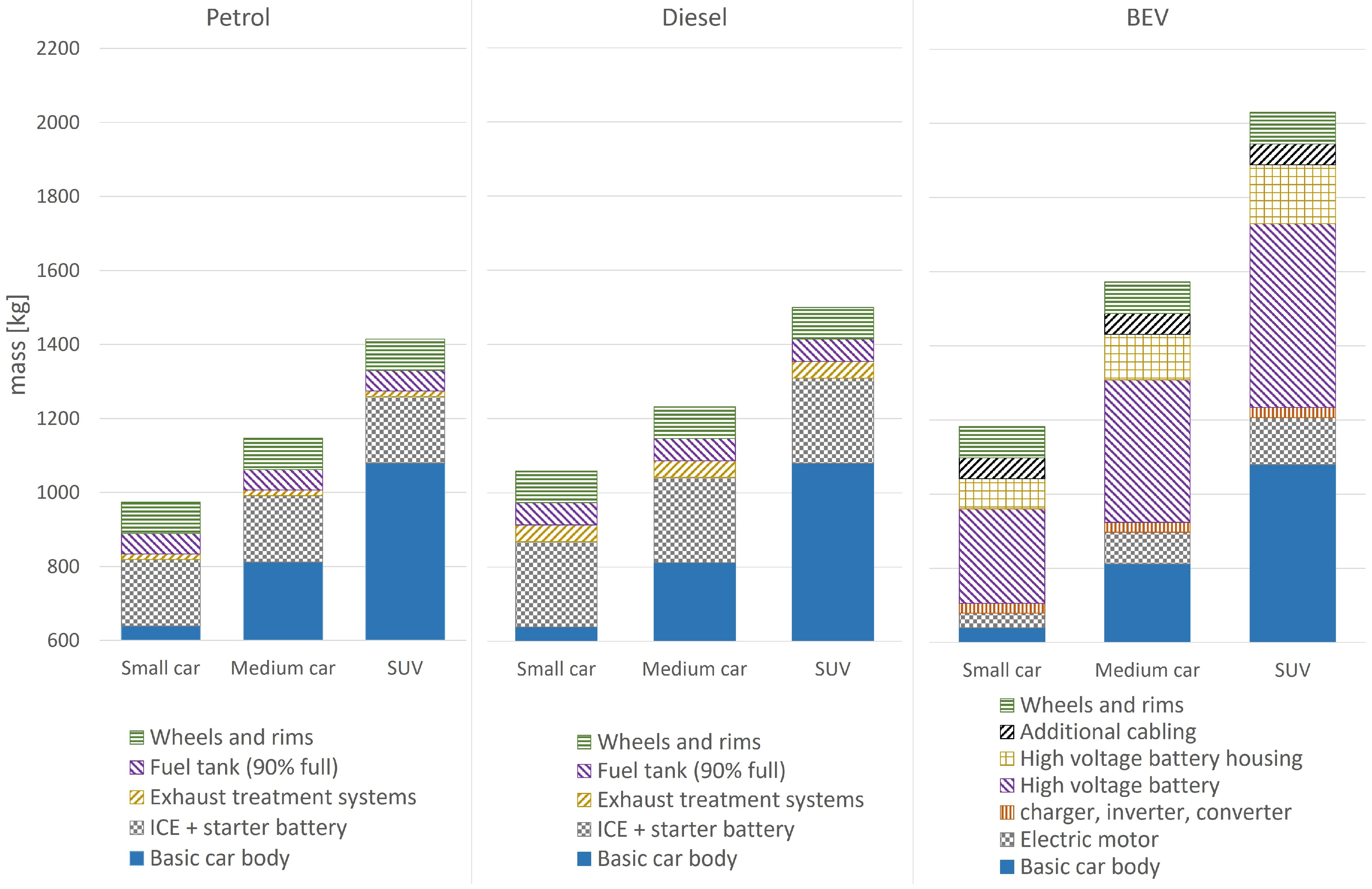
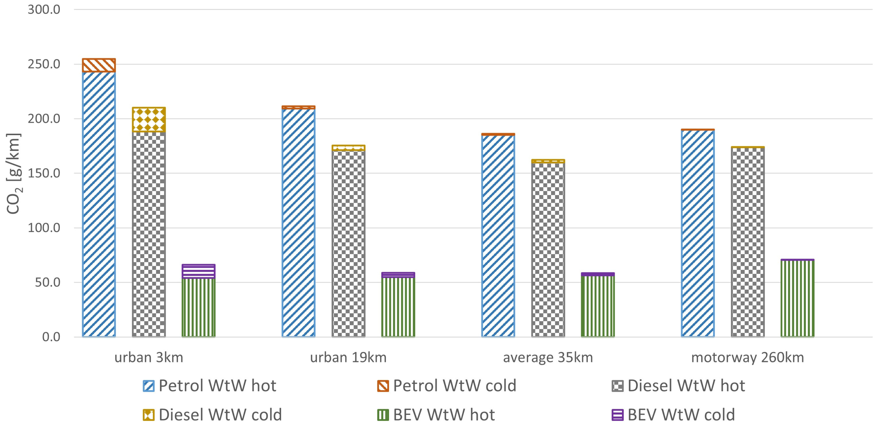
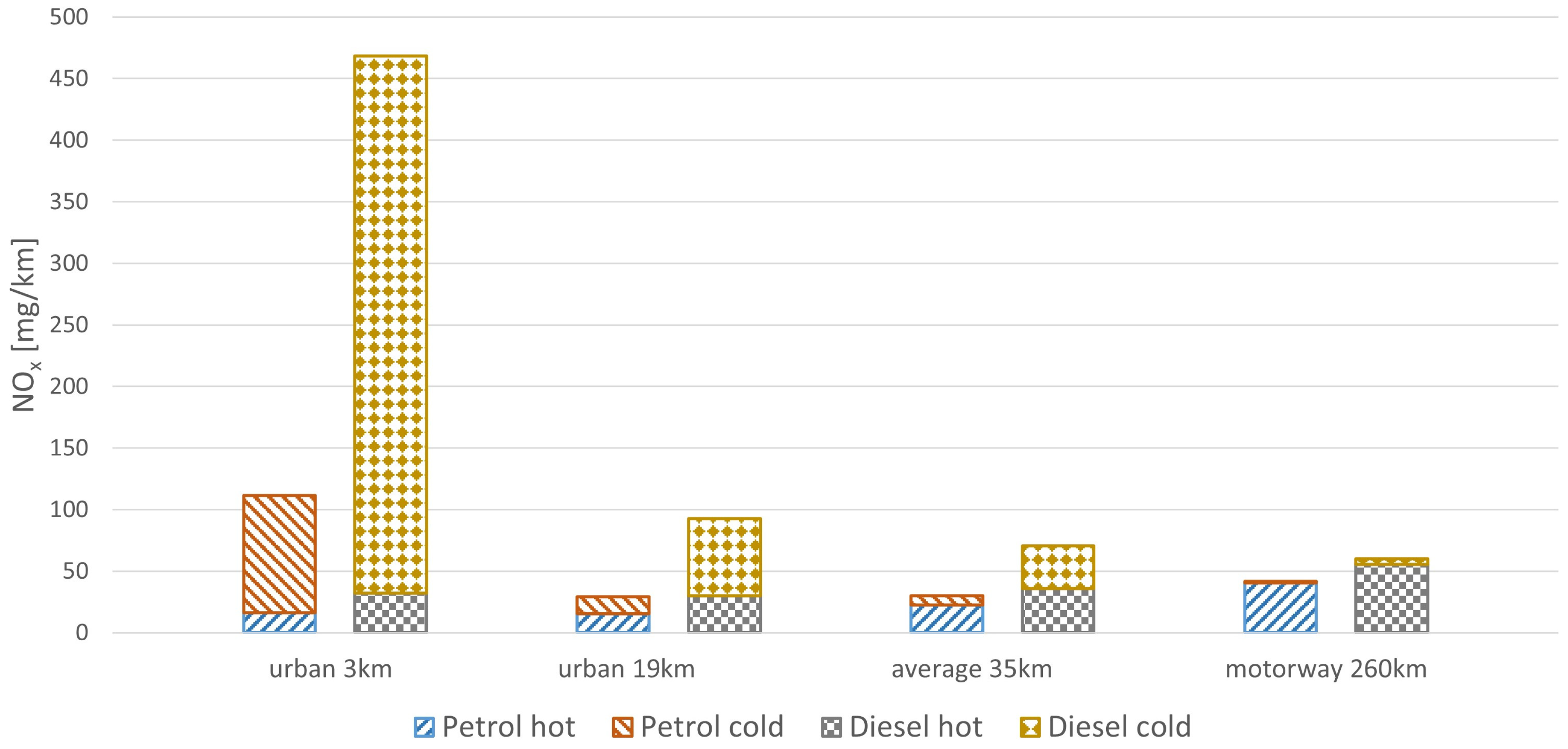