
Dynamic Decoupling Method Based on Motor Dynamic Compensation with Application for Precision Mechatronic Systems

1
Department of Control Science and Engineering, Harbin Institute of Technology, Harbin 150001, China
2
Center of Ultra-Precision Optoelectronic Instrument Engineering, Harbin Institute of Technology, Harbin 150001, China
*
Author to whom correspondence should be addressed.
Energies 2024, 17(9), 2038; https://0-doi-org.brum.beds.ac.uk/10.3390/en17092038
Submission received: 12 March 2024
/
Revised: 3 April 2024
/
Accepted: 10 April 2024
/
Published: 25 April 2024
(This article belongs to the Special Issue Linear/Planar Motors and Other Special Motors)
Abstract
:Motors are widely employed in mechatronic systems, especially in precision multiple degrees of freedom motion systems. In most applications, the dynamic equation between the motor instruction and the actual driving force is simplified as a constant. Subsequently, the static decoupling method can be utilized to design the feedback controller. However, in high-precision mechatronic systems, motor dynamics cannot be neglected, and the static decoupling performance is compromised due to discrepancies between motors. In this paper, a dynamic decoupling method is developed to improve the decoupling performance of the multiple-input multiple-output systems. The effects of transmission delays, motor dynamics, and discrepancies between different motors are taken into consideration in the dynamic decoupling method. Furthermore, a data-driven optimization method is developed to estimate the parameters of the dynamic decoupling controller. The effectiveness and superiority of the proposed method are demonstrated through numerical simulations. The experimental results show that the dynamic decoupling control method can achieve a performance improvement at least compared to the static decoupling control method.
1. Introduction
Multiple degrees of freedom (DoFs) mechatronic systems play a pivotal role in various industrial applications, such as robot manipulators [1], vibration test systems [2], numerical control machine tools [3], applications in the field of energy [4], etc. The parallel design scheme, owing to its spatial and dynamic advantages, is widely adopted in these systems [5]. However, the inherent simplicity of this design introduces challenges, particularly in control aspects, which become more pronounced in applications to achieve high-precision motion, such as the wafer scanner utilized in lithography equipment [6].
To obtain high-precision performance for each degree of freedom (DOF), numerous control strategies have been developed [7], and the decoupling control method emerges as the most widely employed approach. Based on the mechanical structure and operating under the rigid body hypothesis, a static decoupling matrix can be established to effectively decouple the motion of each DOF [8]. Nevertheless, three significant challenges arise in high-precision motion scenarios. Firstly, the static decoupling matrix, which is employed for achieving rigid body decoupling, relies on mechanical structure parameters, including the positions of the center of mass (CoM) and the stress point. Owing to the impact of machining and assembly errors, discrepancies may arise between the utilized parameters and their actual values, resulting in static decoupling errors [9]. Secondly, to achieve high-performance motion in mechatronic systems, high-performance motors, such as linear motors, voice coil motors, and piezoelectric ceramic motors, are often employed as actuators [10]. In the static decoupling method, the characteristics of each motor are considered to be consistent and unchanging during motion. However, owing to variations between different motors and drivers, as well as limitations in magnetic field strength and current loop bandwidth [11], the static decoupling method cannot achieve complete decoupling in essence. Therefore, the decoupling performance of the static decoupling method is compromised. Thirdly, the varying transmission delays across different channels further exacerbate the decoupling effect [12]. Owing to the influences of these factors, the decoupled system using a static decoupling matrix does not exhibit a diagonal form, leading to the emergence of interactions among degrees of freedom, commonly known as cross-talk [13,14]. With increasing accuracy requirements, cross-talk has become a significant impediment to achieving the desired performance in precision mechatronic systems [15].
To eliminate the cross-talk and improve the decoupling performance, various methods have been reported in the literature, which can be categorized into two main approaches. The first approach treats cross-talk as a parasitic dynamic of each DOF, allowing the design of a robust feedback controller to suppress its effects [16]. The most prevalent method within this category is the equivalent transfer function (ETF) method [17]. In the ETF method, the plant to be controlled in each loop is represented by a generalized model when other loops are closed [18]. It is evident that the interactions are taken into account, therefore, a better feedback controller can be designed for improved performance. However, because the generalized plant of each DoF incorporates the influence of controllers from other DoFs, it is complicated to refine the controller when the performance requirement is not satisfied. In [19], an ETF method is proposed, in which the complicated interaction modes are approximated as lower-order equivalent models to simplify the design of the controller. In addition to the ETF method, other robust control methods can be utilized such as the hybrid integrator–gain method, the method, the model predictive control method, etc. [20]. However, since the interactions inevitably increase the complexity of the plant and reduce the attainable bandwidth, only a limited reduction of cross-talk can be obtained. Consequently, the second method, which directly improves the accuracy of decoupling, proves to be the more effective approach in enhancing the performance of precision mechatronic systems.
As highlighted earlier, interactions, stemming from errors in mechanical parameters, variations between motors, and transmission delays, can compromise system performance. Consequently, it becomes imperative to compensate for these factors to achieve full decoupling. Conventionally, mechanical parameters can be calibrated using professional instruments to enhance the accuracy of the static decoupling matrix [21]. However, due to limitations in workspace, certain instruments may no longer be suitable [22]. Furthermore, this indirect optimization method may introduce additional calculation errors in the process. Due to the influence of the other two factors, it can be noted that achieving full decoupling of the system with a static decoupling matrix becomes impractical. Based on the compensation for the inconsistency of motors and transmission channels, a dynamic decoupling controller is proposed in this paper. The dynamic decoupling controller consists of two components: a dynamic component parameterized as a rational transfer function, and a static component. The dynamic component is employed to address inconsistencies between motors and transmission channels, while the static component is utilized to achieve full decoupling of the rigid body of the mechatronic system.
Additionally, to obtain the optimal estimate of the unknown parameter in the dynamic decoupling controller, a data-driven optimization method is developed in this paper, which is inspired by the virtual reference feedback tuning (VRFT) method [23]. The key contributions of this work, in comparison to existing literature, can be succinctly outlined as follows:
- (1)
- A dynamic decoupling control method is established in this paper, based on the compensation for the motor dynamics and the transmission delays.
- (2)
- A data-driven optimization method is developed in this paper to estimate the unknown parameters of the dynamic decoupling controller, requiring only minimal model information. Furthermore, the proposed method is non-iterative, necessitating only a single experiment.
Notations:
Let R be the set of real numbers. For n, a positive integer, is the set of real vectors of dimension n. Vector denotes . For a vector , the i-th element can be denoted as . We define as the norm of vectors, i.e., .
2. Problem Formulation
2.1. Control Configuration of the Multiple DoFs Mechatronic System
We consider a precision multiple DoFs mechatronic system, as depicted in Figure 1, which is a prototype for the short stroke stage of the wafer stage. The prototype shown in Figure 1 consists of a stator and a mover with sufficient stiffness. The mover is driven by three voice coil motors labeled as , , and , respectively, to accomplish nano-scale motion. The voice coil motor can achieve precise and linear motion with high acceleration and high force-to-weight ratio, which render it ideal for applications that require fast and accurate positioning. Three linear encoders are mounted close to the motors; for simplicity, the measurement data of the encoders are supposed to be equal to the displacement distance of the voice coil motors. The target point, defined as the center point of the mover, is controlled to track a predetermined trajectory. The reference trajectory is defined in a Cartesian coordinate system, denoted as , and the displacements of the three degrees of freedom of the target point can be directly obtained as , , and , respectively.
To control the prototype, the decoupling control scheme based on a nominal static decoupling matrix can be utilized, as Figure 2 shows. In this configuration, is the rigid body dynamics model of the mover describing the relationship between the motor driving force and the displacement of the target point. represents the transfer function between motor instruction and motor driving force, which is in the form of a diagonal. is denoted as a transmission delays matrix of three transmission channels from the digit controller to drivers. is the static decoupling matrix to decouple the plant . is the diagonal feedback controller matrix comprised of single-input single-output controllers designed with respect to the desired decoupled system. The signals and are a high-order polynomial trajectory and tracking error, respectively. is the control signal calculated by . and represent the motor instruction and the actual driving force of the motor. is the measured displacement of the target point in coordinate . In addition, the displacements of three voice coil motors can be denoted as , which is not represented in the block diagram. Based on the definitions above, the dynamic model of the control system can be described as follows:
2.2. Description of Nominal Static Decoupling Method
To simplify the controller design, the nominal static decoupling method can be primarily used to stabilize the system. In the static decoupling method, the transmission delays and the motor dynamics are neglected so that and , where I is the identity matrix. The simplified structure of the prototype is shown in Figure 3a, with the nominal mechanical parameters known. From Figure 3a, it can be concluded that the CoM coincides with the target point and the distances between motors and the CoM in the coordinate are , , and , respectively. Under the rigid body hypothesis, the dynamic equations of the motion of the target point can be established as
where , , and are driving forces of three motors, respectively. m is the mass of the mover. and are moment of inertia of and at the CoM, respectively. From (2), can be modeled as
It is evident that is a multivariable system and is not in diagonal form. Directly designing an appropriate feedback controller for such a system is challenging. To apply the static decoupling method, a static decoupling matrix should be employed. Based on the nominal model , the nominal static decoupling matrix can be determined easily as follows:
Consequently, the decoupled system achieves full decoupling, which can be written as
Subsequently, three single-input single-output (SISO) feedback controllers, such as PID controllers, can be easily designed with respect to , , and . However, in the actual system, the actual mechanical parameters may differ from the nominal values, and and cannot be considered static under high precision requirements.
2.3. Formulation of Factors Causing Incomplete Decoupling
As Figure 3b shows, due to errors in manufacturing and assembly, the CoM of the mover no longer coincides with the target point, and the actual installation positions of the motors have also changed. In this situation, the actual rigid body dynamic would no longer be equal to the nominal rigid body dynamic (3), which can be expressed as (6):
where the elements can be detailed as
It is evident that the actual plant cannot be completely decoupled with the nominal decoupling matrix, unless the following equations are satisfied:
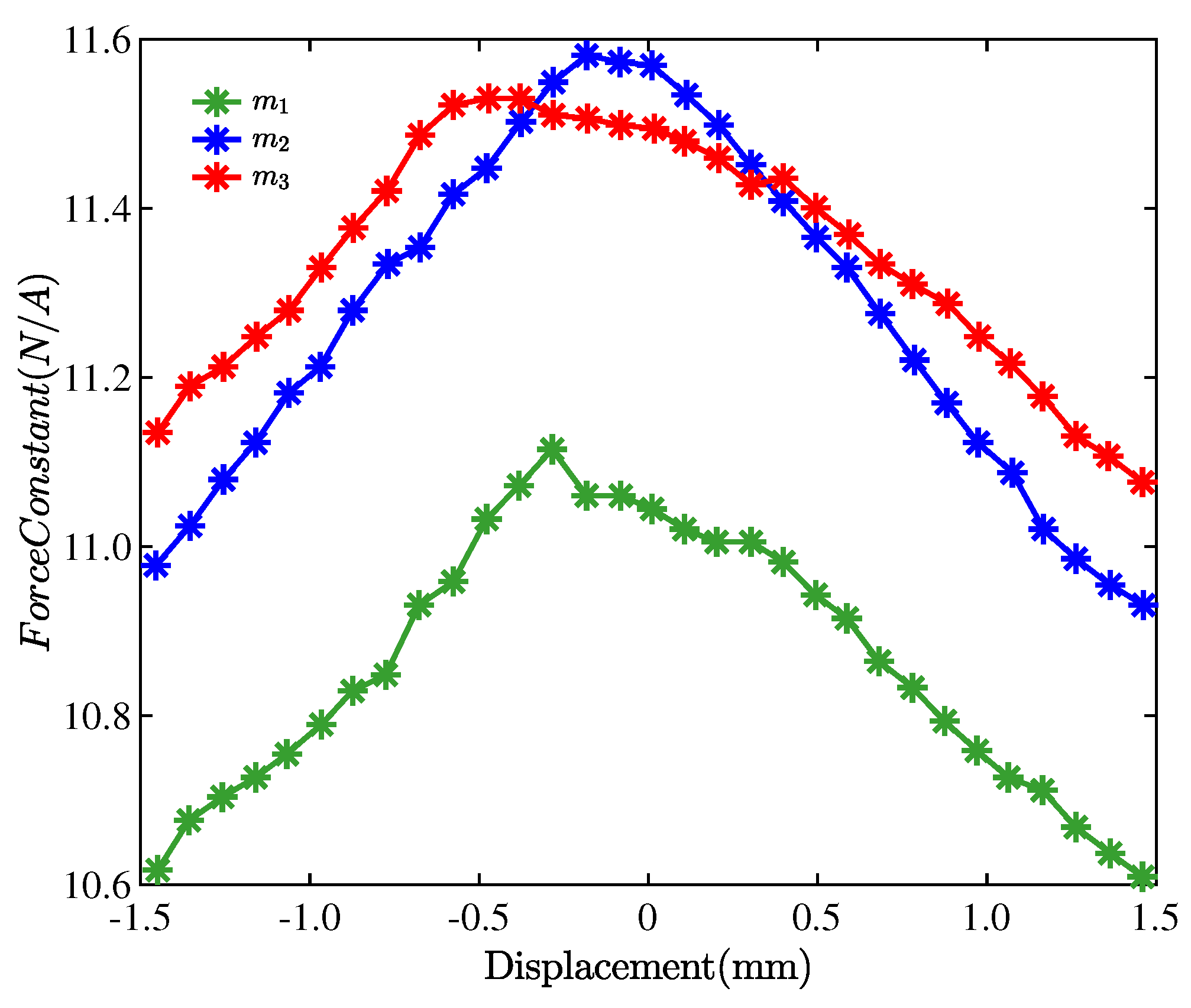
Although the actual system with a nominal decoupling matrix can maintain stability in the case of small errors, it is difficult to obtain the desired performance. Therefore, the decoupling matrix should be improved to enhance the level of decoupling. To decouple the actual rigid body model, the optimal static decoupling matrix can be obtained based on accurate mechanical parameters, such as and , for . However, under the requirements of high speed and high-precision accuracy, the motor dynamics and the transmission delays cannot be neglected. As depicted in Figure 4, with the same coil current input, the static output forces of different motors in different displacements are not constant. Further considering the effect of the motor time constant, the dynamic model of the motor can be expressed as follows:
where is the i-th element of . for , which indicates that the force constant of the motor is related to the displacement of the motor.
On the other hand, the transmission delays matrix can be expressed in detail as
where for represents the delays of different transmission channels.
It can be claimed that, if and only if the following conditions are satisfied, the actual plant can be decoupled by a static decoupling matrix. According to the conditions, Theorem 1 can be established.
Theorem 1.
Proof.
Using proof by contradiction, we suppose that there exists a constant matrix K such that is diagonal, and this can be expressed as
where the j-row elements of can be given as
We denote as the element in the j-th row and i-th column of the inverse matrix of K. Then, can be written as
We suppose that can be expressed as , where and are coprime polynomials and is monic. From (6), the actual rigid body model can be simplified:
Subsequently, the j-th row of can also be determined as
where is the row vector consisting of the elements of the j-th row of .
Therefore, to achieve full decoupling of the actual system with motor dynamics and transmission delays, the static decoupling matrix should be substituted by a dynamic decoupling controller. Based on the above analysis, the ideal dynamic decoupling controller can be determined as the following form:
In order to obtain a parameterized model that is easy to handle, two simplification treatments are applied to and . First, the variant force constants are approximated as polynomials of order of m for . can be written as
where represents the j-th power of and for are unknown coefficients. Then the inverse of can be approximated as
Second, to obtain the an invertible approximation of the pure delays term of , the Pade approximant [24] can be utilized, and the inverse of can be written approximately as
Finally, to ensure the causality of the dynamic decoupling controller, a Q-filter with a relative order of 2 is required, and the desired dynamic decoupling controller based on the compensation of motor dynamics and transmission delays can be parameterized as
where is a known second-order stable polynomial in the s domain. As mentioned above, the unknown parameters of can be determined based on the mechanical parameters, motor dynamics, and transmission delays. However, it is difficult to measure and identify these parameters, and additional errors will be introduced in the final calculation process. To address these problems, an on-line optimization method is developed.
3. Data-Driven Optimization Method
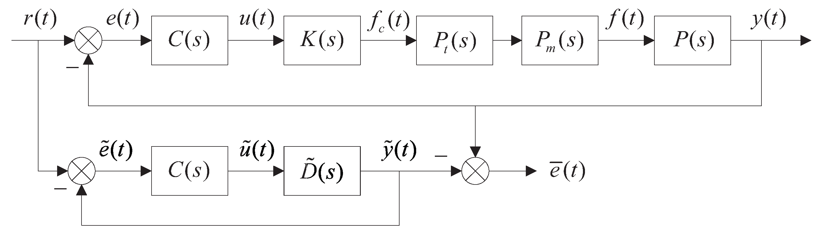
In this section, a data-driven method is proposed to estimate the unknown parameters of the dynamic decoupling controller . The configuration of the proposed method is depicted in Figure 5. As shown in Figure 5, a reference model is used which should be diagonal, and the essential idea is to adjust the parameters of to make the decoupled system as close to as possible.
In other words, if the output of is equal to the output of with the same conditions of reference input and feedback controller, then can be achieved. We suppose that the output of the reference model is equal to ; the output of the feedback controller in reference model can be determined as
From (22), if the output of the feedback controller in the actual system can be equal to by adjusting the parameters of , the following equations can be established:
It is obvious that the decoupled system is completely diagonal if (23) is satisfied. Therefore, the following equivalent objective function can be established, and the optimal estimate of the parameters of can be obtained by minimizing it:
where denotes the -norm of vector x.
Substituting (21) into (24), the objective function J can be derived as
where represents the i-th element of . denotes a row vector consisting of the i-th row elements of . Then, the optimization of J can be achieved by optimizing , , and , respectively.
Substituting (21) into (25), can be parameterized as follows:
where denotes the i-th row of . Since is not equal to 0 and fluctuates less around the nominal value and the minimum of depends on the error term in (26), the minimization of can be equivalent to the minimization of , which can be written as
For the simplicity of expression, we define the following symbols:
Subsequently, (28) can be simplified as
To solve the optimization problem in practice, (30) should be converted to a discrete form
where , , , and are the k-th sampling values of , , , and , respectively and N is the sampling number. For simplicity, we define
Then, the estimate of can be obtained by using the least square method as follows:
The estimate of , , , and can easily obtained based on (29), which can be denoted as , , , and . In addition, the estimate of , and can be obtained as , , and , which can be written as
Finally, the estimate of can be expressed as
4. Simulations Results
In this section, the effectiveness of the proposed method is validated by comparing it with the nominal decoupling method and the ideal static decoupling method, which can decouple the rigid body model of the system in the absence of the motor dynamics and transmission delays. These methods can be represented as follows:
- (1)
- : the nominal static decoupling control method.
- (2)
- : the ideal static decoupling control method.
- (3)
- : the proposed dynamic decoupling control method.
The static decoupling matrices obtained by and are denoted as and , respectively. The dynamic decoupling controller determined by is represented as .
4.1. Simulation Setup
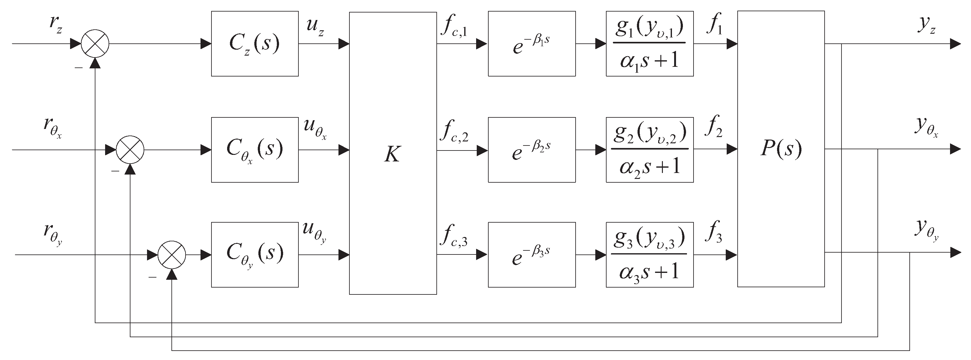
A simulation experiment was conducted to demonstrate the effectiveness of and the simulation block diagram was established, as Figure 6 shows. A fixed step size of was adopted in the numerical calculations of differential equations, and the algorithm of the solver was set to ode4. The total simulation time was set to 1 s, which meant that the sampling number was 5000. The actual values of mechanical parameters in the coordinate are provided in Table 1. We supposed that the mass of the SS stage was and the moment of inertia of and at the CoM were and , respectively. By the rigid body hypothesis, the transfer function model between the driving forces of motors and the three DoFs’ displacement of the target point can be given as
The nominal mechanical parameters presented in Figure 3a are , , and . Based on the nominal mechanical parameters, the nominal static decoupling matrix can be determined as
We specify the desired decoupled model as follows:
Based on the actual rigid body model of the plant and the desired decoupled model, the ideal static decoupling matrix can be determined as
To investigate the effect of motor dynamics and transmission delays, the dynamic equations in the form of (9) and (10) were added into the simulation. The parameters used are listed in Table 2 and Table 3. In the simulation, the variant force constants for different motors were approximated as a polynomial of order 5, according to the measurement data shown in Figure 4. Because these parameters were close to the nominal values, the diagonal dominance of the system could still be ensured by using the nominal static decoupling method when these errors were ignored. Thus, a decentralized controller could be designed to ensure the stability of the system. Nevertheless, due to the inaccurate mechanical parameters, there would have been a great deterioration of performance. To improve the performance of the precision mechatronic system, the dynamic decoupling method proposed in Section 3 can be utilized. In order to estimate the unknown parameters of the dynamic decoupling controller, a data-driven optimization method is developed in Section 4.
To estimate the unknown parameters in , the reference model was selected as , and the order used in (18) was chosen as in the simulation. By conducting excitation experiments on the closed-loop system using , the dynamic decoupling controller could be determined. The estimated results are shown in Table 4 with the Q-filter selected as follows:
4.2. Performance Assessment
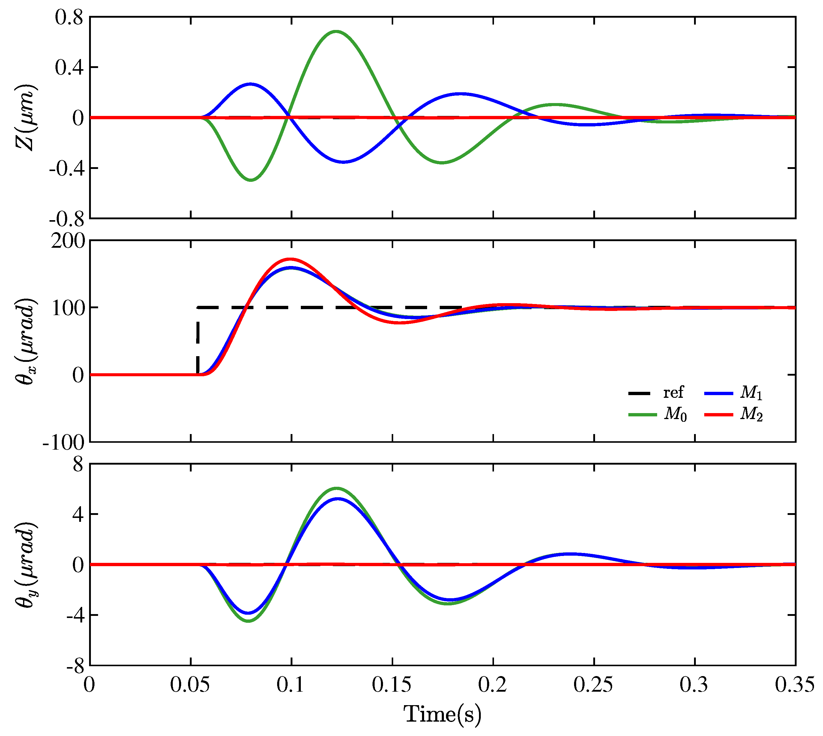
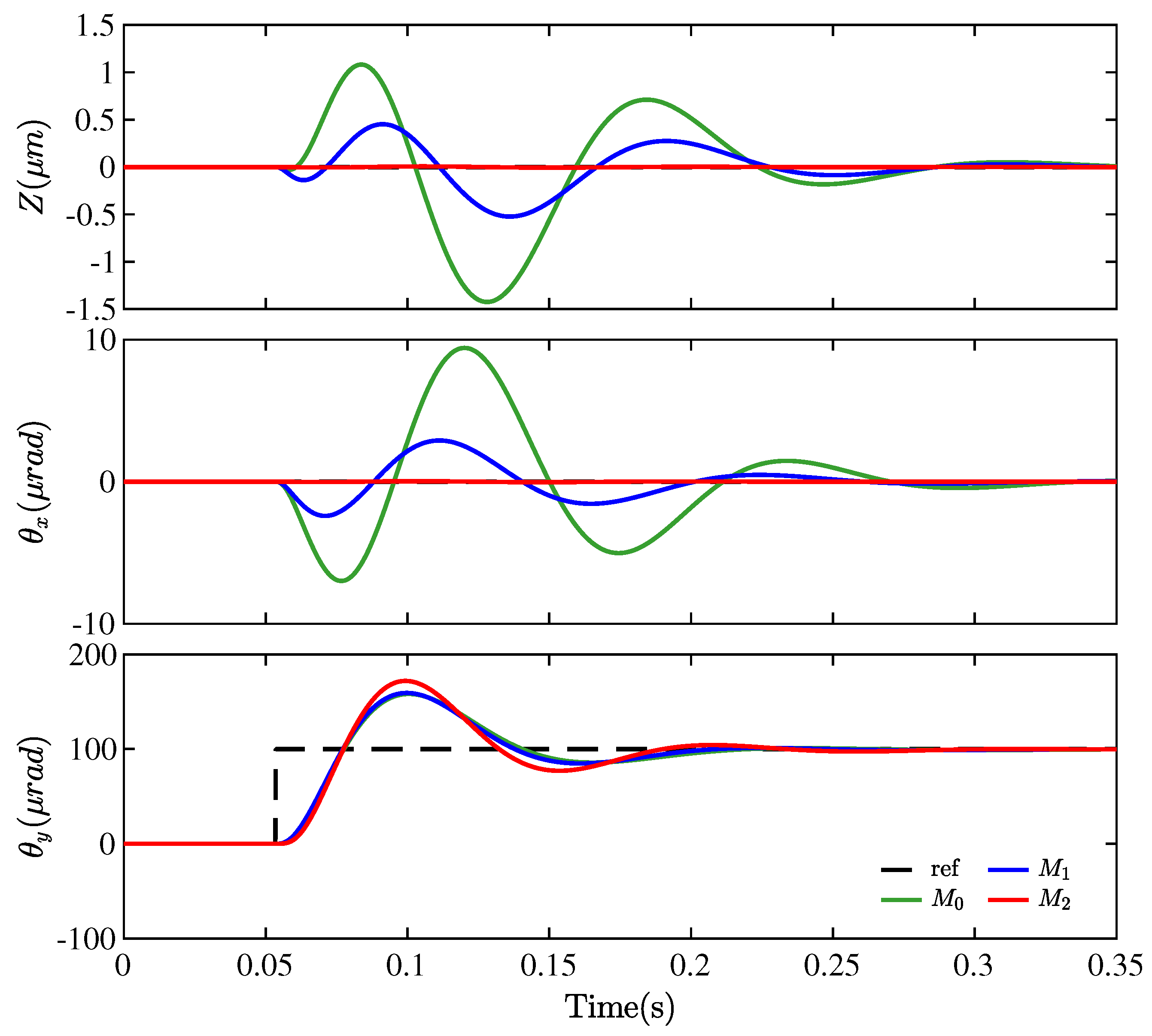
To demonstrate the effectiveness of the dynamic decoupling method more intuitively, some validation experiments in the time domain were carried out. Tracking experiments for three DoFs were conducted for different systems with the same feedback controller. In the first tracking experiment, a step signal of was exerted in z-DoF as the reference input. Similarly, a step signal of was exerted in -DoF and -DoF as the reference input in the second and the third tracking experiments, respectively. It should be noted that in each tracking experiment, the reference inputs of the other two DoFs were set as 0, except the one tracking the step signal. Therefore, the output responses of these DoFs should be 0 when the system is fully decoupled. However, the outputs of the DOFs that track the zero signal were much greater than 0 when using and as shown in Figure 7, Figure 8 and Figure 9. The outputs were derived from the inaccurate decoupling, which can be referred to as the cross-talk. On the contrary, the cross-talk of the decoupled system using was almost negligible. It can be concluded that the decoupling effect of the was the best. Consequently, to quantify the degree of decoupling, the sum of the maximum value of cross-talk can be used as the indicator, which can be denoted as
where are selected in the set of , respectively, is the weighting coefficient, and represents the maximum value of the cross-talk of the j-DoF when the i-DoF is excitated. Based on the maximum value of cross-talk in tracking experiments shown in Table 5, the SAC of different decoupled systems using different decoupling methods can be determined as
where the weighting coefficient is chosen as for . , , and are calculated based on the decoupled system with , , and , respectively. It can be concluded that the dynamic decoupling method proposed in this paper outperforms the other two static decoupling methods, and at least and performance improvements were obtained compared to and , respectively. Consequently, the effectiveness and the superiority of the proposed method can be clearly demonstrated.
5. Conclusions
In this paper, a novel dynamic decoupling method was developed based on the compensation for varying motor dynamics and transmission delays. The key essence of the proposed method lies in the structured dynamic component included in the decoupling controller. What is more, to estimate the unknown parameters, an on-line data-driven optimization algorithm was presented, where only inputs and outputs of the plant need to be measured in a single experiment. Both theoretical analysis and experimental results confirm that the proposed structured dynamic decoupling approach can achieve accurate decoupling; thus, the interactions between multiple DOFs in the mechatronic system can be eliminated significantly. Consequently, compared to the conventional static decoupling methods, a performance improvement can be obtained by the proposed dynamic decoupling method.
Author Contributions
Conceptualization, K.L.; methodology, K.L.; writing—original draft, K.L. and F.S.; software, K.L.; validation, K.L.; investigation, K.L. and Y.L.; supervision, Y.L. and J.T.; project administration, Y.L. and J.T. All authors have read and agreed to the published version of the manuscript.
Funding
This research was funded by the National Natural Science Foundation of China (52075132 and 52105546) and the Opening Foundation of State Key Lab of Digital Manufacturing Equipment & Technology, China (DMETKF2020024).
Data Availability Statement
All data used are contained within the article.
Conflicts of Interest
The authors declare no conflicts of interest.
Abbreviations
The following abbreviations are used in this manuscript:
| CoM | Center of mass |
| DoF | Degree of freedom |
| DoFs | Degrees of freedom |
| ETF | Equivalent transfer function |
| MIMO | Multiple-input multiple output |
| SAC | Sum of the absolute value of the maximum value of cross-talk |
| SISO | Single-input single-output |
| VRFT | Virtual reference feedback tuning |
References
- Incremona, G.P.; Ferrara, A.; Magni, L. MPC for Robot Manipulators With Integral Sliding Modes Generation. IEEE-ASME Trans. Mechatron. 2017, 3, 1299–1307. [Google Scholar] [CrossRef]
- Zheng, Y.; Zhou, Z.; Huang, H. A multi-frequency MIMO control method for the 6DOF micro-vibration exciting system. Acta Astronaut. 2020, 170, 552–569. [Google Scholar] [CrossRef]
- Hanifzadegan, M.; Nagamune, R. Contouring Control of CNC Machine Tools Based on Linear Parameter-Varying Controllers. IEEE-ASME Trans. Mechatron. 2016, 5, 2522–2530. [Google Scholar] [CrossRef]
- Jeon, T.; Kim, D.; Song, Y.; Paek, I. Design and Validation of Demanded Power Point Tracking Control Algorithm for MIMO Controllers in Wind Turbines. Energies 2021, 18, 5818. [Google Scholar] [CrossRef]
- Ma, J.; Cheng, Z.; Zhu, H.; Li, X.; Tomizuka, M.; Lee, T.H. Convex Parameterization and Optimization for Robust Tracking of a Magnetically Levitated Planar Positioning System. IEEE Trans. Ind. Electron. 2022, 4, 3798–3809. [Google Scholar] [CrossRef]
- Song, F.; Liu, Y.; Jin, W.; Tan, J.; He, W. Data-Driven Feedforward Learning With Force Ripple Compensation for Wafer Stages: A Variable-Gain Robust Approach. IEEE Trans. Neural Netw. Learn. Syst. 2022, 4, 1594–1608. [Google Scholar] [CrossRef] [PubMed]
- Schitter, G. Advanced Mechatronics for Precision Engineering and Mechatronic Imaging Systems. IFAC Pap. 2015, 1, 942. [Google Scholar] [CrossRef]
- Butler, H. Position Control in Lithographic Equipment An Enabler for Current-Day Chip Manufacturing. IEEE Control Syst. Mag. 2011, 5, 28–47. [Google Scholar]
- Heertjes, M.; Hennekens, D.; Steinbuch, M. MIMO feed-forward design in wafer scanners using a gradient approximation-based algorithm. Control Eng. Pract. 2010, 5, 495–506. [Google Scholar] [CrossRef]
- Barros, C.P.B.; Butler, H.; van de Wijdeven, J.; Tóth, R. On feedforward control of piezoelectric dual-stage actuator systems. In Proceedings of the 2021 60th IEEE Conference on Decision and Control (CDC), Austin, TX, USA, 14–17 December 2021; pp. 5588–5594. [Google Scholar]
- Poot, M.; Portegies, J.; Mooren, N.; van Haren, M.; van Meer, M.; Oomen, T. Gaussian Processes for Advanced Motion Control. IEEJ J. Ind. Appl. 2022, 3, 396–407. [Google Scholar]
- Li, B.; Zhou, X.; Ning, Z.; Guan, X.; Yiu, K.-F.C. Dynamic event-triggered security control for networked control systems with cyber-attacks: A model predictive control approach. Inf. Sci. 2022, 612, 384–398. [Google Scholar] [CrossRef]
- Zhao, D.; Xia, L.; Dang, H.; Wu, Z.; Li, H. Design and control of air supply system for PEMFC UAV based on dynamic decoupling strategy. Energy Convers. Manag. 2022, 253, 115159. [Google Scholar] [CrossRef]
- Hagglund, T.; Shinde, S.; Theorin, A.; Thomsen, U. An industrial control loop decoupler for process control applications. Control. Eng. Pract. 2022, 123, 105138. [Google Scholar] [CrossRef]
- Heertjes, M.; van Engelen, A. Minimizing cross-talk in high-precision motion systems using data-based dynamic decoupling. Control Eng. Pract. 2011, 12, 1423–1432. [Google Scholar] [CrossRef]
- Shen, Y.; Cai, W.-J.; Li, S. Normalized decoupling control for high-dimensional MIMO processes for application in room temperature control HVAC systems. Control Eng. Pract. 2010, 6, 652–664. [Google Scholar] [CrossRef]
- Luan, X.; Chen, Q.; Liu, F. Equivalent Transfer Function based Multi-loop PI Control for High Dimensional Multivariable Systems. Int. J. Control Autom. Syst. 2015, 2, 346–352. [Google Scholar] [CrossRef]
- Wu, G.; Sun, H.; Zhang, X.; Egea-Alvarez, A.; Zhao, B.; Xu, S.; Wang, S.; Zhou, X. Parameter Design Oriented Analysis of the Current Control Stability of the Weak-Grid-Tied VSC. IEEE Trans. Power Deliv. 2021, 3, 1458–1470. [Google Scholar] [CrossRef]
- Luan, X.; Chen, Q.; Liu, F. Centralized PI control for high dimensional multivariable systems based on equivalent transfer function. ISA Trans. 2014, 5, 1554–1561. [Google Scholar] [CrossRef] [PubMed]
- Rahideh, A.; Bajodah, A.H.; Shaheed, M.H. Real time adaptive nonlinear model inversion control of a twin rotor MIMO system using neural networks. Eng. Appl. Artif. Intell. 2012, 6, 1289–1297. [Google Scholar] [CrossRef]
- van Dael, M.; Witvoet, G.; Swinkels, B.; Oomen, T. Systematic feedback control design for scattered light noise mitigation in Virgo’s MultiSAS. In Proceedings of the 2022 IEEE 17th International Conference on Advanced Motion Control (AMC), Padova, Italy, 18–20 February 2022; pp. 300–305. [Google Scholar]
- Wang, X.; Yang, B.; Zhu, Y. Optimization of current distribution coefficients to decouple the 6-DOF fine stage of lithographic equipment. Optik 2016, 20, 9896–9904. [Google Scholar] [CrossRef]
- Campestrini, L.; Eckhard, D.; Gevers, M.; Bazanella, A.S. Virtual Reference Feedback Tuning for non-minimum phase plants. Automatica 2011, 8, 1778–1784. [Google Scholar] [CrossRef]
- Wang, Y.; Zhang, J.; Zhang, H.; Xie, X. Adaptive Fuzzy Output-Constrained Control for Nonlinear Stochastic Systems with Input Delay and Unknown Control Coefficients. IEEE Trans. Cybern. 2021, 11, 5279–5290. [Google Scholar] [CrossRef] [PubMed]
Figure 1.
The diagram of the prototype of the short stroke stage.

Figure 2.
The configuration of the decoupling control.

Figure 3.
The simplified structure diagrams of the prototype with (a) nominal mechanical parameters and (b) actual mechanical parameters.
Figure 3.
The simplified structure diagrams of the prototype with (a) nominal mechanical parameters and (b) actual mechanical parameters.

Figure 4.
The measured force constants for different motors at different displacements.

Figure 5.
Block diagram of the proposed data-driven optimization method.

Figure 6.
The diagram of the simulation experiment.

Figure 7.
The output responses of tracking experiment of z-DoF.

Figure 8.
The output responses of tracking experiment of -DoF.

Figure 9.
The output responses of tracking experiment of -DoF.


Table 1.
Actual mechanical parameters used in the simulation.
| Points | Values (m) |
|---|---|
Table 2.
Actual parameters of motor dynamics and transmission delays used in the simulation.
| Parameters | Values |
|---|---|
Table 3.
Parameters of the force constant polynomial used in the simulation.
| Parameters | |||
|---|---|---|---|
Table 4.
The estimated results based on the structure of dynamic decoupling controller.
| Parameters | Estimate | Parameters | Estimate | Parameters | Estimate |
|---|---|---|---|---|---|
| −30,359 | |||||
| −41,652 | |||||
| −21,208 |
Table 5.
The maximum value of cross-talk in tracking experiments with different decoupling controllers (matrix).
Table 5.
The maximum value of cross-talk in tracking experiments with different decoupling controllers (matrix).
| Excitated | |||
|---|---|---|---|
| DoF | |||
| z | None 1 | ||
| None | |||
| None | |||
| None | |||
| None | |||
| None | |||
| None | |||
| None | |||
| None |
1 “None” indicates that the data is not relevant to the content of the text.
Disclaimer/Publisher’s Note: The statements, opinions and data contained in all publications are solely those of the individual author(s) and contributor(s) and not of MDPI and/or the editor(s). MDPI and/or the editor(s) disclaim responsibility for any injury to people or property resulting from any ideas, methods, instructions or products referred to in the content. |
© 2024 by the authors. Licensee MDPI, Basel, Switzerland. This article is an open access article distributed under the terms and conditions of the Creative Commons Attribution (CC BY) license (https://creativecommons.org/licenses/by/4.0/).
Share and Cite
MDPI and ACS Style
Liu, K.; Liu, Y.; Song, F.; Tan, J. Dynamic Decoupling Method Based on Motor Dynamic Compensation with Application for Precision Mechatronic Systems. Energies 2024, 17, 2038. https://0-doi-org.brum.beds.ac.uk/10.3390/en17092038
AMA Style
Liu K, Liu Y, Song F, Tan J. Dynamic Decoupling Method Based on Motor Dynamic Compensation with Application for Precision Mechatronic Systems. Energies. 2024; 17(9):2038. https://0-doi-org.brum.beds.ac.uk/10.3390/en17092038
Chicago/Turabian StyleLiu, Kaixin, Yang Liu, Fazhi Song, and Jiubin Tan. 2024. "Dynamic Decoupling Method Based on Motor Dynamic Compensation with Application for Precision Mechatronic Systems" Energies 17, no. 9: 2038. https://0-doi-org.brum.beds.ac.uk/10.3390/en17092038
Note that from the first issue of 2016, this journal uses article numbers instead of page numbers. See further details here.