Passive Super-Twisting Second-Order Sliding Mode Control Strategy for Input Stage of MMC-PET

Abstract

When the operating state of the power system changes, a modular multilevel converter power electronic transformer (MMC-PET) based on modular multilevel converters cannot perform efficient energy transfer and power conversion under conventional control strategies. To address the above problems, this paper proposes a passive, second-order super-helical sliding mode control strategy for MMC-PET by combining passive control and second-order super-helical sliding mode control with a stronger anti-interference capability. First, a Euler–Lagrange model based on positive and negative sequence separation is established according to the mathematical model of the MMC; second, the model of the system is passively analyzed, and a passive controller is designed according to its passivity, and the passive controller is further optimized by using the super-helical second-order sliding mode control, which improves the overall robustness and interference immunity; finally, the effectiveness and superiority of the super-twisting second-order sliding mode passive control strategy is demonstrated by verifying it through the construction of the MMC-PET simulation model and testing it under various non-ideal working conditions.

1. Introduction

Power Electronic Transformers (PETs) are a new type of transformer that combine a high-frequency transformer and a power electronic converter. In addition to the functions of conventional transformers, PETs also have the advantages of realizing instantaneous power regulation and improving power quality. This makes them of great significance in the field of grid-connected distributed energy sources as well as flexible power transmission [1,2,3].

At present, PET research is mainly focused on the improvement of topology and control strategies. With the development of AC/DC power distribution systems towards higher voltage and power, new topologies have emerged, including cascaded H-bridge power electronic transformers, three-level cell power electronic transformers, and others [4,5]. In recent years, the Modular Multilevel Converter (MMC) has been widely studied due to its suitability for high-voltage and large-capacity occasions, strong expandability, and excellent voltage withstand. There is now literature on the combination of MMC and PET to form a new type of topology called Modular Multilevel Converter Power Electronic Transformers (MMC-PET) [6,7]. The power electronic transformer may lose its ideal working environment due to the complexity of the power grid and load. Effective controller design is crucial for ensuring the smooth operation of a power electronic transformer under non-ideal conditions, such as grid voltage disturbance and sudden load changes, which can cause damage to the reliability of the transformer’s operation and the quality of its output power [8,9].

The traditional PI control is commonly used due to its mature theory and simple control parameters. However, under certain operating conditions, such as unbalanced power grid disturbances and the integration of power electronic devices, the traditional PI control may suffer from low control accuracy and poor dynamic performance [10,11]. To address these issues, scholars have introduced nonlinear control strategies. Nonlinear control offers strong adaptivity and accurate signal tracking, making it more suitable for addressing system stability issues under non-ideal working conditions and improving system dynamic performance. In reference [12], PI-based fuzzy logic control was applied to MMC-PET for grid voltage dips, resulting in improved ability to cope with voltage dips and harmonic handling. However, it should be noted that the fuzzy control relied on a rule table developed based on experience. Reference [13] applied a combination of PIR control and model predictive control (MPC) in MMC. The PIR-MPC control method eliminates the weighting factor and simplifies the control’s complexity. However, this method requires real-time tracking of the current and is less effective in controlling unstable systems. Reference [14] proposed an improved droop control based on cascade-type PET. This method enhances the accuracy of system voltage control and regulation under dynamics without affecting the original control framework. However, the article did not conduct comparative experiments to verify its superiority.

All other control strategies mentioned above start with the signal, while passivity-based control takes a different approach. Passivity-based control is a nonlinear strategy that analyzes the system’s energy and structural characteristics to improve the asymptotic speed of the system’s function by injecting appropriate damping. This is a current research topic [15,16]. References [17,18,19] implemented passivity-based control on power electronic devices, including MMC, power spring, and photovoltaic inverter, to enhance their response speed, output quality, and system stability. However, passivity-based control is susceptible to interference and cannot adjust to parameter changes under non-ideal operating conditions. Sliding mode control is a control strategy that is known for its robustness in countering the effects of external disturbances and internal parameters. This is achieved by presetting the trajectory of the objective function and changing the control structure based on the system’s state when it is running under non-ideal operating conditions [20,21]. However, the control volume of traditional sliding mode control is discontinuous. This discontinuity causes the system state to traverse back and forth on the expected state trajectory, forming the phenomenon of buffeting when the state volume is close to the sliding mode surface. This buffeting may lead to the system failing to converge [22,23]. Reference [24] compared the conventional sliding mode control with the Super-Twisting second-order sliding mode control and confirmed the superiority of the latter in addressing the buffeting. In a similar vein, Reference [25] utilized the Super-Twisting second-order sliding mode control for vehicle travel distance control, resulting in improved stability and robustness of the control.

Based on the aforementioned studies, this paper proposes a passive super-twisting second-order sliding mode control strategy for MMC-PET. The established mathematical model is first separated into positive and negative sequences, and a passive controller based on Euler–Lagrange (EL) is designed according to its passivity. Then, a super-twisting second-order sliding-mode control is adopted to optimize the passive controller and enhance the overall steady state performance of the system, providing stronger anti-interference ability and smaller buffeting. Finally, a simulation model of MMC-PET is established, and the experimental results of PI control, passive control, and second-order sliding mode control are compared to verify the effectiveness and feasibility of the control strategy under different operating conditions.

2. MMC-PET System Structure and Input Stage Mathematical Modeling

2.1. MMC-PET System Structure

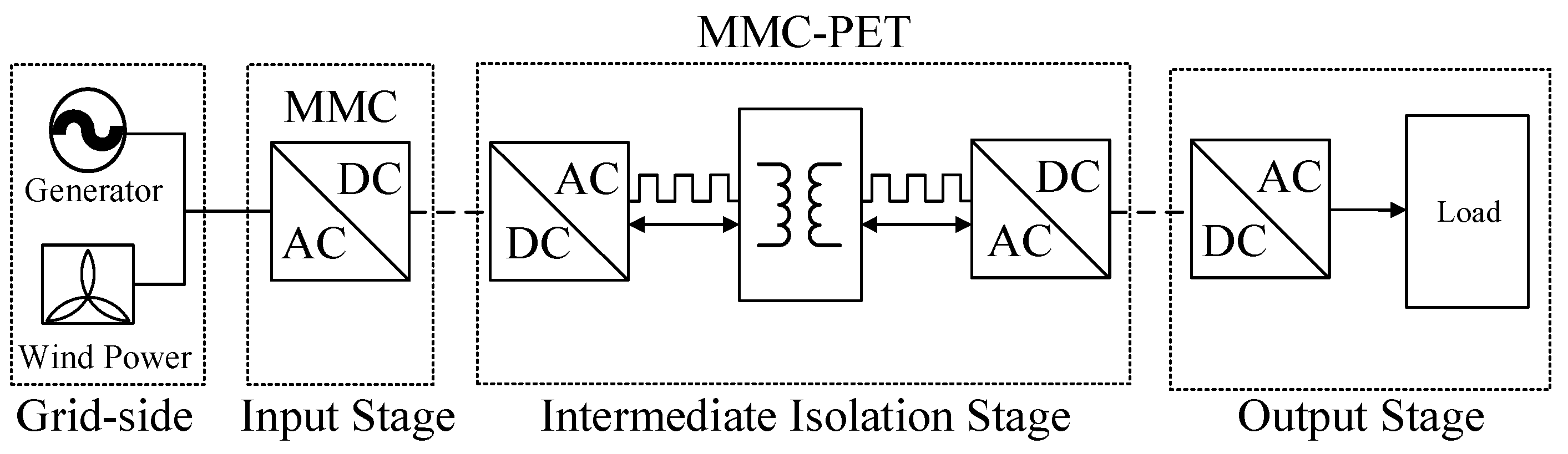
The overall system structure of a three-stage modular multilevel power electronic transformer is shown in Figure 1.

The MMC-PET topology consists of three relatively independent stages: the input stage, the intermediate isolation stage, and the output stage. The input stage serves as the MMC rectifier, which converts high-voltage AC power from the grid-side generator or wind turbine into high-voltage DC power. The intermediate isolation stage comprises several Input Series Output Parallel (ISOP) DC/DC converters. These converters are connected to the input and output stages through the high-voltage and low-voltage DC buses, respectively. Their function is to convert the high-voltage DC output from the input stage to low-voltage DC. The output stage comprises a conventional three-phase inverter that converts the low-voltage DC output from the intermediate isolation stage into AC for direct use by low-voltage equipment and loads.

2.2. Mathematical Modeling of the MMC-PET Input Stage

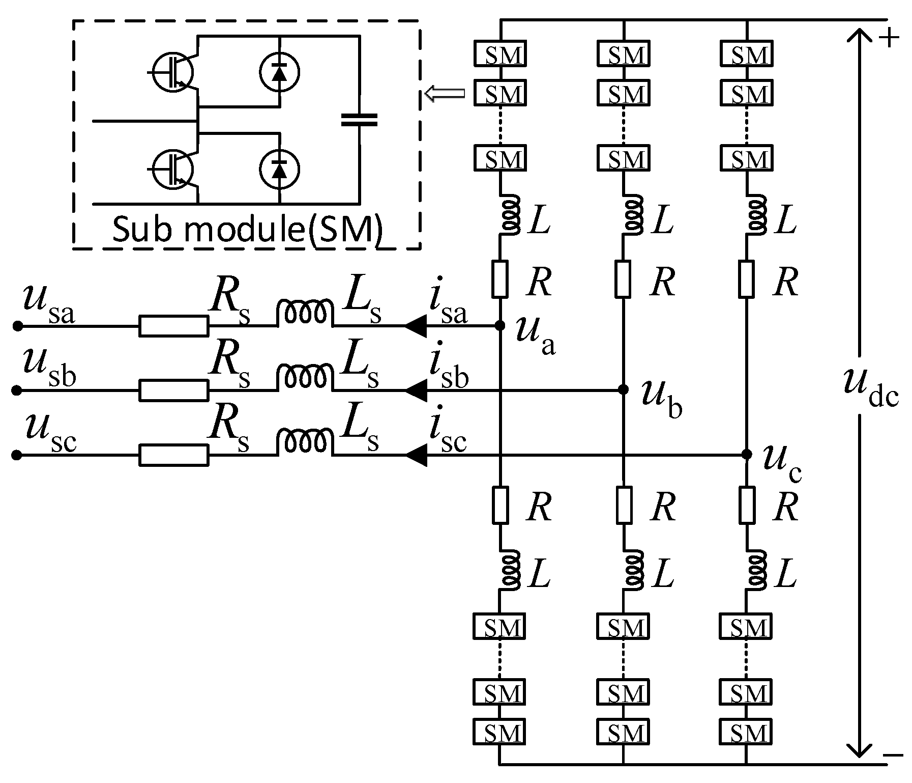
The rectified MMC topology of the MMC-PET input stage is shown in Figure 2.

The Modular Multilevel Converter (MMC) is composed of three-phase six-bridge arms. Each arm comprises N sub-modules (SM) with an identical structure and a bridge inductor, and the upper and lower bridge arms of each phase unit are the same. In this paper, the half-bridge SM is used due to its high efficiency, low cost, and fewer switching devices. The bridge arm inductor is utilized to suppress the phase-to-phase loop current caused by voltage fluctuations in the SM capacitor.

In Figure 2, $u_{\mathrm{sj}}$ is the grid-side three-phase ac voltage; $i_{\mathrm{sj}}$ is the grid-side three-phase current; $u_{\mathrm{j}}$ is the rectifier-side three-phase ac voltage; $u_{\mathrm{d}\mathrm{c}}$ is the dc-side voltage; $R_{\mathrm{s}}$, $L_{\mathrm{s}}$, respectively, is the grid-side resistance and inductance; $R$ and $L$, respectively, is the MMC bridge arm resistance and inductance ($\mathrm{j}=a,b,c$).

Following Kirchhoff’s theorem, the mathematical model of the MMC-PET input stage in the abc three-phase stationary coordinate system can be obtained from Figure 2:

$$\left\{\begin{array}{l}{u}_{\mathrm{sa}}=u_{\mathrm{a}}+(L_{\mathrm{s}}+\frac{L}{2})\frac{\mathrm{d}{i}_{\mathrm{sa}}}{\mathrm{d}t}+(R_{\mathrm{s}}+\frac{R}{2})i_{\mathrm{sa}}\\ u_{\mathrm{sb}}=u_{\mathrm{b}}+(L_{\mathrm{s}}+\frac{L}{2})\frac{\mathrm{d}{i}_{\mathrm{sb}}}{\mathrm{d}t}+(R_{\mathrm{s}}+\frac{R}{2})i_{\mathrm{sb}}\\ u_{\mathrm{sc}}=u_{\mathrm{c}}+(L_{\mathrm{s}}+\frac{L}{2})\frac{\mathrm{d}{i}_{\mathrm{sc}}}{\mathrm{d}t}+(R_{\mathrm{s}}+\frac{R}{2})i_{\mathrm{sc}}\end{array}\right.$$

(1)

To facilitate subsequent analysis and control, (1) undergoes a synchronous rotational transformation. In non-ideal states, the three-phase grid will have a negative sequence component. Therefore, the mathematical model in the dq two-phase rotating coordinate system is separated from the positive and negative sequences to obtain:

$$\left\{\begin{array}{l}{u}_{\mathrm{sd}}^{+}=u_{\mathrm{d}}^{+}-\omega L_{\mathrm{eq}}{i}_{\mathrm{q}}^{+}+L_{\mathrm{eq}}\frac{\mathrm{d}{i}_{\mathrm{d}}^{+}}{\mathrm{d}t}+R_{\mathrm{eq}}{i}_{\mathrm{d}}^{+}\\ u_{\mathrm{sq}}^{+}=u_{\mathrm{q}}^{+}+\omega L_{\mathrm{eq}}{i}_{\mathrm{d}}^{+}+L_{\mathrm{eq}}\frac{\mathrm{d}{i}_{\mathrm{q}}^{+}}{\mathrm{d}t}+R_{\mathrm{eq}}{i}_{\mathrm{q}}^{+}\end{array}\right.$$

(2)

$$\left\{\begin{array}{l}{u}_{\mathrm{sd}}^{-}=u_{\mathrm{d}}^{-}+\omega L_{\mathrm{eq}}{i}_{\mathrm{q}}^{-}+L_{\mathrm{eq}}\frac{\mathrm{d}{i}_{\mathrm{d}}^{-}}{\mathrm{d}t}+R_{\mathrm{eq}}{i}_{\mathrm{d}}^{-}\\ u_{\mathrm{sq}}^{-}=u_{\mathrm{q}}^{-}-\omega L_{\mathrm{eq}}{i}_{\mathrm{d}}^{-}+L_{\mathrm{eq}}\frac{\mathrm{d}{i}_{\mathrm{q}}^{-}}{\mathrm{d}t}+R_{\mathrm{eq}}{i}_{\mathrm{q}}^{-}\end{array}\right.$$

(3)

where $u_{\mathrm{sd}}^{+}$, $u_{\mathrm{sq}}^{+}$, $u_{\mathrm{d}}^{+}$, $u_{\mathrm{q}}^{+}$, $i_{\mathrm{d}}^{+}$, $i_{\mathrm{q}}^{+}$ represent the positive sequence component in the dq two-phase rotating coordinate system for $u_{\mathrm{sj}}$, $u_{\mathrm{j}}$, $i_{\mathrm{sj}}$, respectively. Similarly, $u_{\mathrm{sd}}^{-}$, $u_{\mathrm{sq}}^{-}$, $u_{\mathrm{d}}^{-}$, $u_{\mathrm{q}}^{-}$, $i_{\mathrm{d}}^{-}$, $i_{\mathrm{q}}^{-}$ represent the negative sequence component in the dq two-phase rotating coordinate system for $u_{\mathrm{sj}}$, $u_{\mathrm{j}}$, $i_{\mathrm{sj}}$, respectively. $\omega$ represents the grid fundamental angular frequency, $\omega =2\pi f$; and $L_{\mathrm{e}\mathrm{q}}=L_{\mathrm{s}}+L/2,R_{\mathrm{e}\mathrm{q}}=R_{\mathrm{s}}+R/2$.

3. Control Strategy for the MMC-PET Input Stage

In this section, we derive the passive control rate based on the mathematical model of the MMC-PET input stage and prove the system’s stability under passivity-based control. We then introduce the super-twisting second-order sliding mode control, based on passivity-based control, to obtain the final passive super-twisting second-order sliding mode control rate.

3.1. Passive Controller Design Based on E-L Modeling

The system’s state variables are chosen as follows:

$${\mathit{x}}^{+}=\left[\begin{array}{l}{i}_{\mathrm{d}}^{+}\\ i_{\mathrm{q}}^{+}\end{array}\right] {\mathit{x}}^{-}=\left[\begin{array}{l}{i}_{\mathrm{d}}^{-}\\ i_{\mathrm{q}}^{-}\end{array}\right]$$

(4)

The E-L model in the dq coordinate system is obtained by rewriting (2) and (3) according to (5):

$$\mathit{M}\dot{\mathit{x}}+\mathit{J}\mathit{x}+\mathit{R}\mathit{x}=\mathit{u}$$

(5)

$$\left\{\begin{array}{l}\mathit{M}{\dot{\mathit{x}}}^{+}+{\mathit{J}}^{+}{\mathit{x}}^{+}+\mathit{R}{\mathit{x}}^{+}={\mathit{u}}^{+}\\ \mathit{M}{\dot{\mathit{x}}}^{-}+{\mathit{J}}^{-}{\mathit{x}}^{-}+\mathit{R}{\mathit{x}}^{-}={\mathit{u}}^{-}\end{array}\right.$$

(6)

where, $\mathit{M}$ is the inertia matrix of each phase of the energy storage element ${\mathit{J}}^{+}$, ${\mathit{J}}^{-}$ is the antisymmetric matrix reflecting the coupling relationship within the system; $\mathit{R}$ is the positive definite symmetric matrix of the energy dissipation within the system; ${\mathit{u}}^{+}$, ${\mathit{u}}^{-}$ is the control variable of the energy exchange within and outside the system; and the expression of each matrix is:

$$\mathit{M}=\left[\begin{array}{cc}{L}_{\mathrm{eq}}& 0\\ 0& L_{\mathrm{eq}}\end{array}\right], {\mathit{J}}^{+}=\left[\begin{array}{cc}0& -\omega L_{\mathrm{eq}}\\ \omega L_{\mathrm{eq}}& 0\end{array}\right], {\mathit{J}}^{-}=\left[\begin{array}{cc}0& \omega L_{\mathrm{eq}}\\ -\omega L_{\mathrm{eq}}& 0\end{array}\right], R=\left[\begin{array}{cc}{R}_{\mathrm{eq}}& 0\\ 0& R_{\mathrm{eq}}\end{array}\right], {\mathit{u}}^{+}=\left[\begin{array}{l}{u}_{\mathrm{sd}}^{+}-u_{\mathrm{d}}^{+}\\ u_{\mathrm{sq}}^{+}-u_{\mathrm{q}}^{+}\end{array}\right], {\mathit{u}}^{-}=\left[\begin{array}{l}{u}_{\mathrm{sd}}^{-}-u_{\mathrm{d}}^{-}\\ u_{\mathrm{sq}}^{-}-u_{\mathrm{q}}^{-}\end{array}\right]$$

The multiple-input, multiple-output system can be expressed as follows:

$$\left\{\begin{array}{l}\dot{\mathit{x}}=f(\mathit{x},\mathit{u})\\ \mathit{y}=h(\mathit{x})\end{array}\right., \mathit{x}(0)={\mathit{x}}_0\in R^{\mathrm{n}}$$

(7)

where $\mathit{x}\in R^{\mathrm{n}}$ represents the order of the state vector, $\mathit{u}\in R^{\mathrm{m}}$ represents the order of input vectors, and $\mathit{y}\in R^{\mathrm{m}}$ represents the order of output vectors. The system’s local Lipschitz function is denoted by $f$.

According to the strict passive definition of the system, the dissipation inequality is satisfied when there is a continuously differentiable semi-positive definite storage function $H(\mathit{x})$ and a positive definite function $Q(\mathit{x})$ at any given time t > 0:

$$H(\mathit{x}(t))-H(\mathit{x}(0))\le {\displaystyle {\int }_0^{\mathrm{t}}{\mathit{u}}^{\mathrm{T}}\mathit{y}}d\tau -{\displaystyle {\int }_0^{\mathrm{t}}Q(\mathit{x})}d\tau$$

(8)

Or:

$$\dot{H}(\mathit{x})\le {\mathit{u}}^{\mathrm{T}}\mathit{y}-Q(\mathit{x})$$

(9)

The system is considered strictly passive. The energy storage function is defined as:

$$\left\{\begin{array}{l}{H}^{+}({\mathit{x}}^{+})=\frac{1}{2}{({\mathit{x}}^{+})}^{\mathrm{T}}\mathit{M}{\mathit{x}}^{+}\\ H^{-}({\mathit{x}}^{-})=\frac{1}{2}{({\mathit{x}}^{-})}^{\mathrm{T}}\mathit{M}{\mathit{x}}^{-}\end{array}\right.$$

(10)

By deriving (10) and substituting it into (6), we obtain:

$$\left\{\begin{array}{l}{\dot{H}}^{+}({\mathit{x}}^{+})={({\mathit{x}}^{+})}^{\mathrm{T}}\mathit{M}{\dot{\mathit{x}}}^{+}={({\mathit{x}}^{+})}^{\mathrm{T}}{\mathit{u}}^{+}-{({\mathit{x}}^{+})}^{\mathrm{T}}\mathit{R}{\mathit{x}}^{+}\\ {\dot{H}}^{-}({\mathit{x}}^{-})={({\mathit{x}}^{-})}^{\mathrm{T}}\mathit{M}{\dot{\mathit{x}}}^{-}={({\mathit{x}}^{-})}^{\mathrm{T}}{\mathit{u}}^{-}-{({\mathit{x}}^{-})}^{\mathrm{T}}\mathit{R}{\mathit{x}}^{-}\end{array}\right.$$

(11)

Setting the variables in (11):

$$\left\{\begin{array}{l}{\mathit{y}}^{+}={\mathit{x}}^{+},Q({\mathit{x}}^{+})={({\mathit{x}}^{+})}^{\mathrm{T}}\mathit{R}{\mathit{x}}^{+}\\ {\mathit{y}}^{-}={\mathit{x}}^{-},Q({\mathit{x}}^{-})={({\mathit{x}}^{-})}^{\mathrm{T}}\mathit{R}{\mathit{x}}^{-}\end{array}\right.$$

(12)

After simplifying Equation (11), it becomes evident that Equation (9) is satisfied, indicating that the MMC-PET input stage system meets the strict passive definition.

Under non-ideal conditions, the reference values of the state variables for positive and negative sequence separation in the system are:

$${{\mathit{x}}^{*}}^{+}=\left[\begin{array}{l}{i}_{\mathrm{dref}}^{+}\\ i_{\mathrm{qref}}^{+}\end{array}\right], {{\mathit{x}}^{*}}^{-}=\left[\begin{array}{l}{i}_{\mathrm{dref}}^{-}\\ i_{\mathrm{qref}}^{-}\end{array}\right]$$

(13)

Subtracting the actual state variable from the desired state variable yields the error variable:

$$\left\{\begin{array}{l}{\mathit{x}}_{\mathrm{e}}^{+}={\mathit{x}}^{+}-{({\mathit{x}}^{+})}^{*}\\ {\mathit{x}}_{\mathrm{e}}^{-}={\mathit{x}}^{-}-{({\mathit{x}}^{-})}^{*}\end{array}\right.$$

(14)

The E-L model of the error variable can be obtained by substituting (14) into (6):

$$\left\{\begin{array}{l}\mathit{M}{\dot{\mathit{x}}}_{\mathrm{e}}^{+}+J^{+}{\mathit{x}}_{\mathrm{e}}^{+}+\mathit{R}{\mathit{x}}_{\mathrm{e}}^{+}={\mathit{u}}^{+}-(\mathit{M}{{\dot{\mathit{x}}}^{*}}^{+}+{\mathit{J}}^{+}{{\mathit{x}}^{*}}^{+}+\mathit{R}{{\mathit{x}}^{*}}^{+})\\ \mathit{M}{\dot{\mathit{x}}}_{\mathrm{e}}^{-}+{\mathit{J}}^{-}{\mathit{x}}_{\mathrm{e}}^{-}+\mathit{R}{\mathit{x}}_{\mathrm{e}}^{-}={\mathit{u}}^{-}-(\mathit{M}{{\dot{\mathit{x}}}^{*}}^{-}+{\mathit{J}}^{-}{{\mathit{x}}^{*}}^{-}+\mathit{R}{{\mathit{x}}^{*}}^{-})\end{array}\right.$$

(15)

The error variable’s energy storage function is selected as:

$$\left\{\begin{array}{l}{\mathit{H}}^{+}({\mathit{x}}_{\mathrm{e}}^{+})=\frac{1}{2}{({\mathit{x}}_{\mathrm{e}}^{+})}^{\mathrm{T}}\mathit{M}{\mathit{x}}_{\mathrm{e}}^{+}\\ {\mathit{H}}^{-}({\mathit{x}}_{\mathrm{e}}^{-})=\frac{1}{2}{({\mathit{x}}_{\mathrm{e}}^{-})}^{\mathrm{T}}\mathit{M}{\mathit{x}}_{\mathrm{e}}^{-}\end{array}\right.$$

(16)

Under passive control, the system’s state variables will converge infinitely to the reference value, and the error energy storage function will converge to 0. At $\mathrm{t}\to \infty$, we obtain the E-L mathematical model of the error variable.

$$\left\{\begin{array}{l}\mathit{M}{\dot{\mathit{x}}}_{\mathrm{e}}^{+}+J^{+}{\mathit{x}}_{\mathrm{e}}^{+}+\mathit{R}{\mathit{x}}_{\mathrm{e}}^{+}=0\\ \mathit{M}{\dot{\mathit{x}}}_{\mathrm{e}}^{-}+{\mathit{J}}^{-}{\mathit{x}}_{\mathrm{e}}^{-}+\mathit{R}{\mathit{x}}_{\mathrm{e}}^{-}=0\end{array}\right.$$

(17)

Using (16) and substituting it with (17) results in:

$$\left\{\begin{array}{l}{\dot{\mathit{H}}}^{+}({\mathit{x}}_{\mathrm{e}}^{+})={({\mathit{x}}_{\mathrm{e}}^{+})}^{\mathrm{T}}\mathit{M}{\dot{\mathit{x}}}_{\mathrm{e}}^{+}=-{({\mathit{x}}_{\mathrm{e}}^{+})}^{\mathrm{T}}\mathit{R}{\mathit{x}}_{\mathrm{e}}^{+}\\ {\dot{\mathit{H}}}^{-}({\mathit{x}}_{\mathrm{e}}^{-})={({\mathit{x}}_{\mathrm{e}}^{-})}^{\mathrm{T}}\mathit{M}{\dot{\mathit{x}}}_{\mathrm{e}}^{-}=-{({\mathit{x}}_{\mathrm{e}}^{-})}^{\mathrm{T}}\mathit{R}{\mathit{x}}_{\mathrm{e}}^{-}\end{array}\right.$$

(18)

According to (18), $\mathit{R}$ determines the rate of convergence of the error energy storage function. The value of $\mathit{R}$ is a fixed impedance value of the lossy devices inside the system, and the value of $\mathit{R}$ is small. Therefore, appropriate damping should be injected into (18) to improve the energy dissipation rate of the system. The damping dissipation term is taken as follows:

$$\left\{\begin{array}{l}{\mathit{R}}_{\mathrm{d}}^{+}{\mathit{x}}_{\mathrm{e}}^{+}=(\mathit{R}+{\mathit{R}}_{\mathrm{a}}^{+}){\mathit{x}}_{\mathrm{e}}^{+}\\ {\mathit{R}}_{\mathrm{d}}^{-}{\mathit{x}}_{\mathrm{e}}^{-}=(\mathit{R}+{\mathit{R}}_{\mathrm{a}}^{-}){\mathit{x}}_{\mathrm{e}}^{-}\end{array}\right.$$

(19)

${\mathit{R}}_{\mathrm{a}}^{+}$, ${\mathit{R}}_{\mathrm{a}}^{-}$ is a positive, definite damping matrix:

$${\mathit{R}}_{\mathrm{a}}^{+}=\left[\begin{array}{cc}{\mathit{R}}_{\mathrm{a}1}^{+}& 0\\ 0& {\mathit{R}}_{\mathrm{a}2}^{+}\end{array}\right], {\mathit{R}}_{\mathrm{a}}^{-}=\left[\begin{array}{cc}{\mathit{R}}_{\mathrm{a}1}^{-}& 0\\ 0& {\mathit{R}}_{\mathrm{a}2}^{-}\end{array}\right]$$

Substituting (19) into (15) provides the improved passive control rate:

$$\left\{\begin{array}{l}{\mathit{u}}^{+}=\mathit{M}{{\dot{\mathit{x}}}^{*}}^{+}+{\mathit{J}}^{+}{{\mathit{x}}^{*}}^{+}+\mathit{R}{{\mathit{x}}^{*}}^{+}-{\mathit{R}}_{\mathrm{a}}^{+}{\mathit{x}}_{\mathrm{e}}^{+}\\ {\mathit{u}}^{-}=\mathit{M}{{\dot{\mathit{x}}}^{*}}^{-}+{\mathit{J}}^{-}{{\mathit{x}}^{*}}^{-}+\mathit{R}{{\mathit{x}}^{*}}^{-}-{\mathit{R}}_{\mathrm{a}}^{-}{\mathit{x}}_{\mathrm{e}}^{-}\end{array}\right.$$

(20)

The final expression for the passivity-based controller can be obtained by expanding the equation as follows:

$$\left\{\begin{array}{l}{u}_{\mathrm{d}}^{+}=u_{\mathrm{sd}}^{+}+\omega L_{\mathrm{eq}}{i}_{\mathrm{qref}}^{+}-R_{\mathrm{eq}}{i}_{\mathrm{dref}}^{+}+R_{\mathrm{a}1}^{+}(i_{\mathrm{d}}^{+}-i_{\mathrm{dref}}^{+})\\ u_{\mathrm{q}}^{+}=u_{\mathrm{sq}}^{+}-\omega L_{\mathrm{eq}}{i}_{\mathrm{dref}}^{+}-R_{\mathrm{eq}}{i}_{\mathrm{qref}}^{+}+R_{\mathrm{a}2}^{+}(i_{\mathrm{q}}^{+}-i_{\mathrm{qref}}^{+})\\ u_{\mathrm{d}}^{-}=u_{\mathrm{sd}}^{-}-\omega L_{\mathrm{eq}}{i}_{\mathrm{qref}}^{-}-R_{\mathrm{eq}}{i}_{\mathrm{dref}}^{-}+R_{\mathrm{a}1}^{-}(i_{\mathrm{d}}^{-}-i_{\mathrm{dref}}^{-})\\ u_{\mathrm{q}}^{-}=u_{\mathrm{sq}}^{-}+\omega L_{\mathrm{eq}}{i}_{\mathrm{dref}}^{-}-R_{\mathrm{eq}}{i}_{\mathrm{qref}}^{-}+R_{\mathrm{a}2}^{-}(i_{\mathrm{q}}^{-}-i_{\mathrm{qref}}^{-})\end{array}\right.$$

(21)

3.2. Passive Super-Twisting Second-Order Sliding Mode Controller Design

Passivity-based control has a limitation in that its control rate is derived from an accurate mathematical model of the system. However, non-ideal working conditions may occur during the actual operation process, causing certain parameters and equilibrium points of the system to change and affect the effectiveness of passive control. Therefore, it is necessary to optimize the passive control rate. Sliding mode control has the advantages of strong anti-interference ability and robustness. However, the control rate of the traditional sliding mode controller contains discretized high-frequency switching terms $sign(s)$, which results in unavoidable buffeting problems for the system-controlled quantities. Therefore, the text utilizes super-twisting second-order sliding mode control to optimize the passive control rate while suppressing the buffeting problem of traditional sliding mode control.

The super-twisting control algorithm can be expressed as follows:

$$\left\{\begin{array}{l}u=u_1+u_2\\ u_1=-\lambda {\left|s\right|}^{\rho }sign(s)\\ u_2=-{\displaystyle \int \alpha sign(s)dt}\\ \dot{u}=-\alpha sign(s)\end{array}\right.$$

(22)

The given equation shows that the first part $u_1$ is a continuous function of the sliding mode surface, while the second part $u_2$ is the integral of the sliding mode surface over time. $s$ represents the sliding mode surface, $\rho$, $\lambda$ and $\alpha$ are the control parameters that need to be satisfied:

$$\left\{\begin{array}{l}{\lambda }^2\ge \frac{4\phi \Gamma (\alpha +\phi )}{{\Gamma }^3(\alpha -\phi )}\\ \alpha >\frac{\phi }{\Gamma }\\ 0<\rho \le 0.5\end{array}\right.$$

(23)

where $\phi$ and $\Gamma$ are the two generalized unknown bounds in the variables, and usually $\phi$ and $\Gamma$ are constants greater than 0. When $\rho$ is taken as 0.5, the system will maximize the possibility of achieving second-order sliding modes.

Based on analysis (22), it is evident that the discretized high-frequency switching term $sign(s)$ is integrated over time for the sliding mode surface, resulting in a continuous form in the control rate. This approach avoids the direct impact of $sign(s)$ on the control rate. The super-twisting control algorithm maintains the benefits of sliding-mode control while eliminating buffeting. It does not necessitate a convergence law $\dot{s}$ and can be controlled directly from the sliding-mode surface $s$.

The current error is chosen to be the sliding mold surface:

$$\left\{\begin{array}{l}{s}_1=i_{\mathrm{d}}^{+}-i_{\mathrm{dref}}^{+},s_2=i_{\mathrm{q}}^{+}-i_{\mathrm{qref}}^{+}\\ s_3=i_{\mathrm{d}}^{-}-i_{\mathrm{dref}}^{-},s_4=i_{\mathrm{q}}^{-}-i_{\mathrm{qref}}^{-}\end{array}\right.$$

(24)

The positive sequence can be taken, for example, to derive (25):

$$\left\{\begin{array}{l}{\dot{s}}_1={\dot{i}}_{\mathrm{d}}^{+}-{\dot{i}}_{\mathrm{dref}}^{+}=\frac{d{i}_{\mathrm{d}}^{+}}{dt}\\ {\dot{s}}_2={\dot{i}}_{\mathrm{q}}^{+}-{\dot{i}}_{\mathrm{qref}}^{+}=\frac{d{i}_{\mathrm{q}}^{+}}{dt}\end{array}\right.$$

(25)

The control rate for super-twisting second-order sliding mode is chosen as the reaching law of the sliding mode surface:

$$\left\{\begin{array}{l}{\dot{s}}_1=-{\lambda }_1{\left|s_1\right|}^{\frac{1}{2}}sign(s_1)-{\displaystyle \int {\alpha }_{1}sign(s_1)dt}\\ {\dot{s}}_2=-{\lambda }_2{\left|s_2\right|}^{\frac{1}{2}}sign(s_2)-{\displaystyle \int {\alpha }_{2}sign(s_2)dt}\end{array}\right.$$

(26)

The combination of (2), (26) and (27) results in:

$$\left\{\begin{array}{l}{u}_{\mathrm{d}}^{+}=u_{\mathrm{sd}}^{+}+\omega L_{\mathrm{eq}}{i}_{\mathrm{q}}^{+}-R_{\mathrm{eq}}{i}_{\mathrm{d}}^{+}+\\ L_{\mathrm{eq}}[{\lambda }_1{\left|s_1\right|}^{\frac{1}{2}}sign(s_1)+{\displaystyle \int {\alpha }_{1}sign(s_1)dt}]\\ u_{\mathrm{q}}^{+}=u_{\mathrm{sq}}^{+}-\omega L_{\mathrm{eq}}{i}_{\mathrm{d}}^{+}-R_{\mathrm{eq}}{i}_{\mathrm{q}}^{+}+\\ L_{\mathrm{eq}}[{\lambda }_2{\left|s_2\right|}^{\frac{1}{2}}sign(s_2)+{\displaystyle \int {\alpha }_{2}sign(s_2)dt}]\end{array}\right.$$

(27)

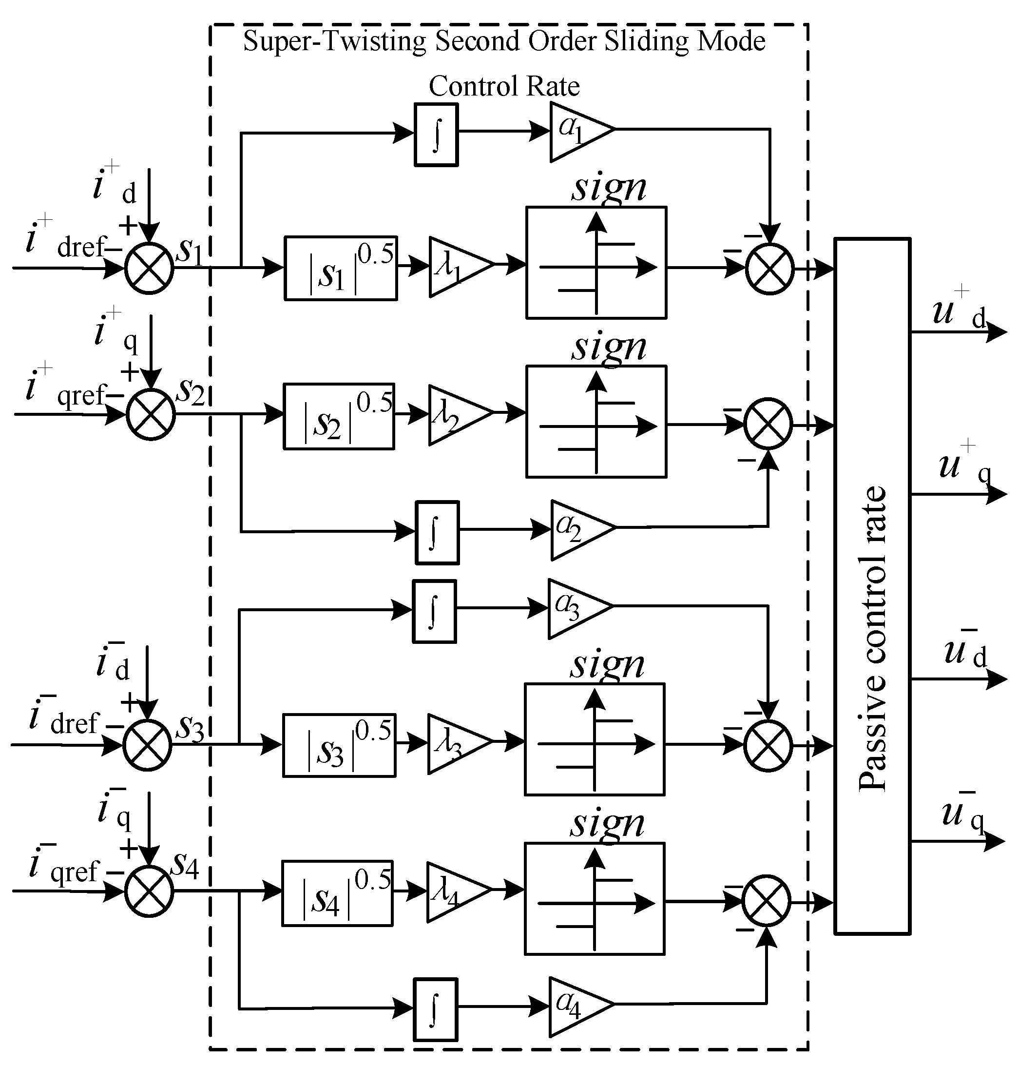
By combining (21) and (27), the control rate of the passive super-twisting second-order sliding mode under the positive sequence system is obtained:

$$\left\{\begin{array}{r}{u}_{\mathrm{d}}^{+}=u_{\mathrm{sd}}^{+}-R_{\mathrm{eq}}{i}_{\mathrm{dref}}^{+}+\frac{\omega L_{\mathrm{eq}}{R}_{\mathrm{a}1}^{+}}{R + R_{\mathrm{a}1}^{+}}{i}_{\mathrm{q}}^{+}+\frac{\omega L_{\mathrm{eq}}R}{R + R_{\mathrm{a}1}^{+}}{i}_{\mathrm{qref}}^{+} +\\ \frac{L_{\mathrm{eq}}{R}_{\mathrm{a}1}^{+}}{R + R_{\mathrm{a}1}^{+}}[{\lambda }_1{\left|s_1\right|}^{\frac{1}{2}}sign(s_1)+{\displaystyle \int {\alpha }_{1}sign(s_1)dt}]\\ u_{\mathrm{q}}^{+}=u_{\mathrm{sq}}^{+}-R_{\mathrm{eq}}{i}_{\mathrm{qref}}^{+}-\frac{\omega L_{\mathrm{eq}}{R}_{\mathrm{a}2}^{+}}{R + R_{\mathrm{a}2}^{+}}{i}_{\mathrm{d}}^{+}-\frac{\omega L_{\mathrm{eq}}R}{R + R_{\mathrm{a}2}^{+}}{i}_{\mathrm{dref}}^{+} +\\ \frac{L_{\mathrm{eq}}{R}_{\mathrm{a}2}^{+}}{R + R_{\mathrm{a}2}^{+}}[{\lambda }_2{\left|s_2\right|}^{\frac{1}{2}}sign(s_2)+{\displaystyle \int {\alpha }_{2}sign(s_2)dt}]\end{array}\right.$$

(28)

Similarly, (29) gives the control rate of a negative sequence, and Figure 3 shows the specific structure of the controller.

$$\left\{\begin{array}{r}{u}_{\mathrm{d}}^{-}=u_{\mathrm{sd}}^{-}-R_{\mathrm{eq}}{i}_{\mathrm{dref}}^{-}-\frac{\omega L_{\mathrm{eq}}{R}_{\mathrm{a}1}^{-}}{R + R_{\mathrm{a}1}^{-}}{i}_{\mathrm{q}}^{-}-\frac{\omega L_{\mathrm{eq}}R}{R + R_{\mathrm{a}1}^{-}}{i}_{\mathrm{qref}}^{-} +\\ \frac{L_{\mathrm{eq}}{R}_{\mathrm{a}1}^{-}}{R + R_{\mathrm{a}1}^{-}}[{\lambda }_3{\left|s_3\right|}^{\frac{1}{2}}sign(s_3)+{\displaystyle \int {\alpha }_{3}sign(s_3)dt}]\\ u_{\mathrm{q}}^{-}=u_{\mathrm{sq}}^{-}-R_{\mathrm{eq}}{i}_{\mathrm{qref}}^{-}+\frac{\omega L_{\mathrm{eq}}{R}_{\mathrm{a}2}^{-}}{R + R_{\mathrm{a}2}^{-}}{i}_{\mathrm{d}}^{-}+\frac{\omega L_{\mathrm{eq}}R}{R + R_{\mathrm{a}2}^{+}}{i}_{\mathrm{dref}}^{-} +\\ \frac{L_{\mathrm{eq}}{R}_{\mathrm{a}2}^{-}}{R + R_{\mathrm{a}2}^{-}}[{\lambda }_4{\left|s_4\right|}^{\frac{1}{2}}sign(s_4)+{\displaystyle \int {\alpha }_{4}sign(s_4)dt}]\end{array}\right.$$

(29)

To ensure feasibility and stability of the passive super-twisting second-order sliding mode control, we use the Lyapunov stability criterion to determine the sliding mode surface.

Setting the Lyapunov function as:

$$V=\frac{1}{2}{s}_1^2$$

(30)

The derivation of the above equation gives:

$$\stackrel{·}{V}=\stackrel{·}{s_1}{s}_1=-s_1({\lambda }_1{\left|s_1\right|}^{\frac{1}{2}}sign(s_1)+{\displaystyle \int {\alpha }_{1}sign(s_1)dt})$$

(31)

To achieve global asymptotic stability of the system, we apply the Lyapunov stability criterion. When $s_1=0$, the system remains stable. When $s_1\ne 0$, the system is in an unstable state. In order to stabilize the system, it needs to ensure that $\stackrel{·}{V}<0$, which control parameters ${\lambda }_1,{\alpha }_1$ are both greater than 0.

3.3. Overall Control Block Diagram of MMC-PET Input Stage

Based on the above analysis, the overall control block diagram of the MMC-PET input stage can be obtained as shown in Figure 4. Figure 4 shows that the control system is mainly composed of positive and negative sequence component separation, dq transformation, current setpoint calculation, passive super-twisting second-order sliding mode controller, sub-module capacitor balancing control, loop current suppression, and modulation module. The specific control process is as follows: first, the grid-side voltage $U_{\mathrm{sabc}}$ and the grid-side current $i_{\mathrm{sabc}}$ are separated from the positive and negative sequences and transformed by dq to obtain the voltage components $U_{\mathrm{sd}}^{+},U_{\mathrm{sq}}^{+},U_{\mathrm{sd}}^{-},U_{\mathrm{sq}}^{-}$ and the current components $i_{\mathrm{d}}^{+},i_{\mathrm{q}}^{+},i_{\mathrm{d}}^{-},i_{\mathrm{q}}^{-}$ in the dq coordinates; second, the current components are calculated by the current reference value to obtain the reference current. The reference current, voltage component, and current component are applied to (28) and (29) for passive super-twisting second-order sliding mode control, and the controlled voltage signal is inverted by dq transformation to obtain the equivalent three-phase output voltage $U_{\mathrm{abc}}$; finally, $U_{\mathrm{f}}$ obtained after submodule capacitor voltage balancing control and loop current suppression, and the output voltage $U_{\mathrm{abc}}$ are jointly modulated with the CPSPWM to generate the control signals that control the submodules of the MMC-PET input stage.

4. Control Strategies for the MMC-PET Intermediate Isolation Stage and Output Stages

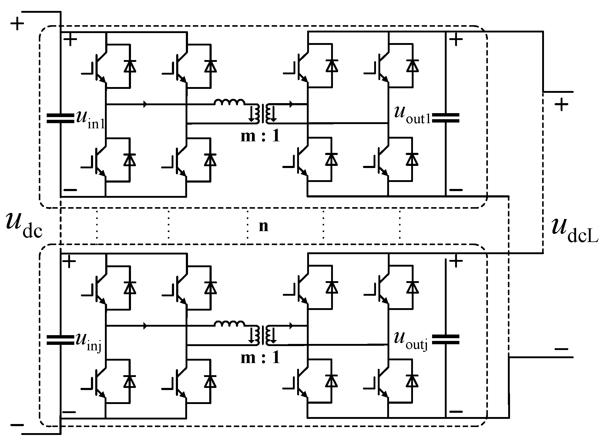
The rectified DC voltage must be voltage converted to obtain different voltage levels, and the DC-DC conversion is realized by an intermediate isolation stage. The topology of the MMC-PET intermediate isolation stage is shown in Figure 5, which is obtained by connecting the input side of several Dual Active Bridge (DAB) converters in series and the output side in parallel. In Figure 4, $u_{\mathrm{dc}}$ is the DC voltage obtained after rectifying the output stage of the MMC-PET; $u_{\mathrm{dcL}}$ is the DC voltage output from the intermediate stage of the MMC-PET; $u_{\mathrm{inj}}$ is the input voltage of the DAB; and $u_{\mathrm{outj}}$ is the output voltage of the DAB ($\mathrm{j}=1,2,\dots ,n$).

In order to ensure the consistency of the input voltage when each DAB operates, the intermediate stage in this paper adopts the input voltage equalization control strategy. First, the reference value $u_{\mathrm{dcL}}^{*}$ of the output voltage of the intermediate stage is compared with the actual output voltage $u_{\mathrm{dcL}}$ of the intermediate stage, and the reference value ${\theta }_{\mathrm{ref}}$ of the DAB drive signal is obtained after PI control; secondly, the average value of the input voltage $u_{\mathrm{dc}}/n$ of the intermediate stage is compared with the actual input voltage $u_{\mathrm{inj}}$ of each DAB, and the correction amount $\Delta {\theta }_{\mathrm{j}}$ of the DAB drive signal is obtained after PI control. After comparing the reference value ${\theta }_{\mathrm{ref}}$ with the correction value $\Delta {\theta }_{\mathrm{j}}$, the drive signal ${\theta }_{\mathrm{j}}$ of the DAB can be obtained, and its control block diagram is shown in Figure 6.

The output stage of MMC-PET adopts a three-phase full-bridge inverter circuit, and the output stage adopts double-loop control. The outer loop voltage and reactive power are controlled by PI to obtain the current reference value, and the difference between the current reference value and the current of the output stage is used to obtain the error signal. The inner loop of the current adopts passivity-based control, which will not be discussed here.

5. Simulation Analysis

To verify the superiority of the passive super-twisting second-order sliding mode control strategy (PBC-SW-SOSMC) based on MMC-PET, we constructed a simulation model of MMC-PET and its control system on the MATLAB/Simulink (R2018b) platform. We tested the system under three operating conditions: changes in loads on the grid-side, temporary voltage unbalance, and non-linear load connections. Simulation experiments were conducted to compare PI control, passive control (PBC), and second-order sliding mode control (SOSMC) with PBC-SW-SOSMC. The specific experimental parameters are listed in

Table 1. System simulation parameters.

	Parameter	Value
Input stage	Grid-side voltage/kV	66
	Grid-side resistance/$\Omega$	0.4
	Grid-side Inductance/mH	0.002
	Number of bridge arm submodules	50
	Bridge arm resistors/$\Omega$	0.01
	Bridge arm Inductance/mH	0.15
	Submodule Capacitance/μF	0.0105
	DC side voltage reference value/kV	135
Intermediate isolation stage	High-voltage side capacitor/mF	1
	Low-voltage side capacitor/mF	8
	Rated Ratio	7:1
	Rated frequency/Hz	50
Output stage	Submodule Capacitance/μF	0.01
	Voltage Frequency/Hz	50
	Voltage amplitude/kV	18
	Bridge arm resistors/$\Omega$	0.1

.

5.1. Grid-Side Load Change

For the grid-side load change experiment, a 15 Ω resistor was added to the gird side and controlled using a time-delay switch. The load change time was set to 0.8~1.3 s, with the load being cut in at 0.8 s and cut out at 1.3 s, lasting for 0.5 s. The experimental results are presented in Figure 7, Figure 8 and Figure 9.

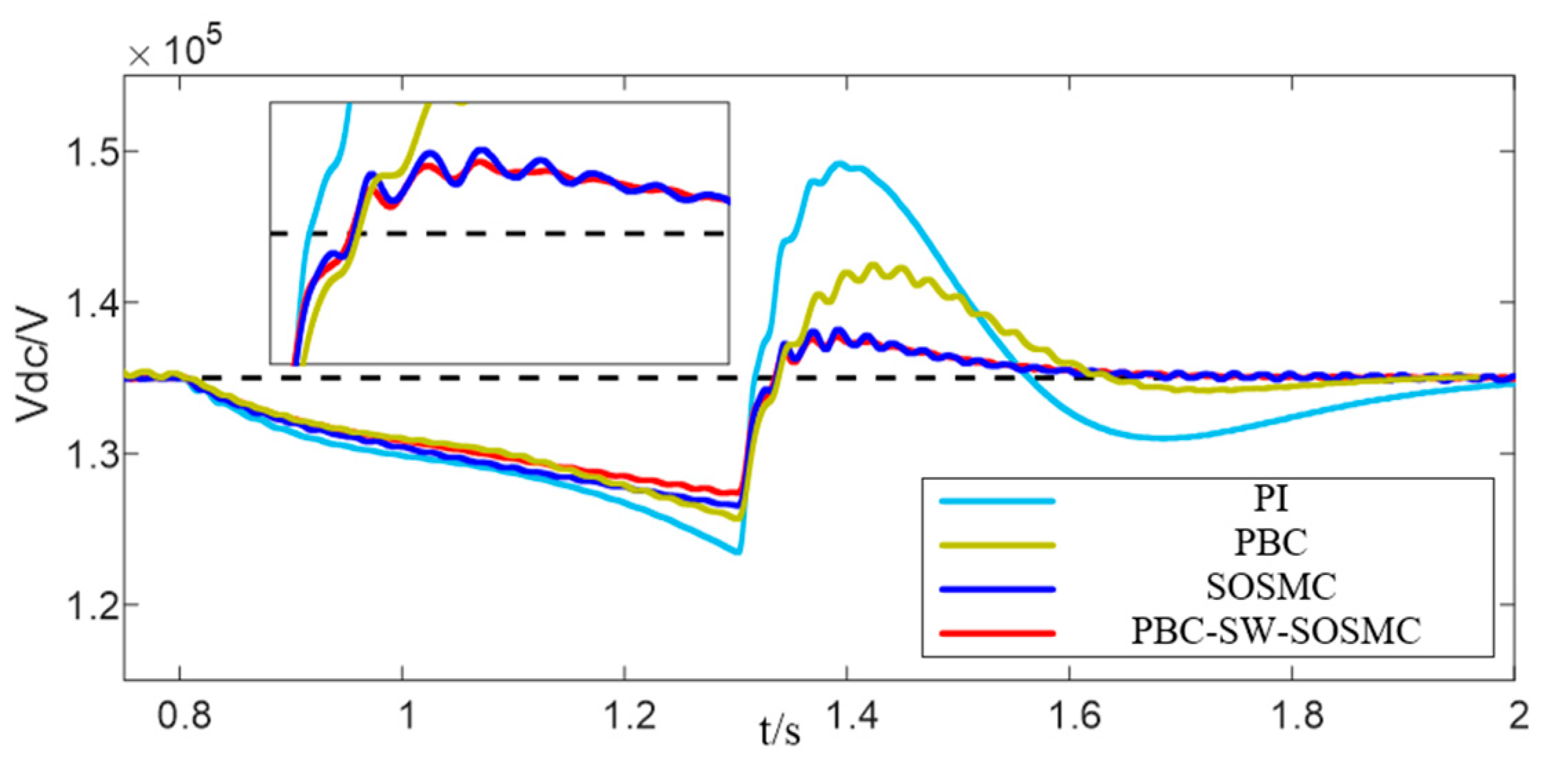
Figure 7 displays the simulation waveforms of the MMC-PET high DC side voltage. As shown in the figure, the high DC side voltage experiences a transient drop at 0.8 s due to a sudden change in load on the grid side. The voltage then gradually recovers and stabilizes after the load is removed at 1.3 s. Under PI control, the high DC voltage transiently dropped by a larger value, and there was also an overshoot of about 15,000 V after 1.3 s, which stabilized only after 0.7 s. The overall control effect was not satisfactory. Although the control effectiveness is improved by the PBC and SOSMC, the waveforms exhibit different degrees of high frequency oscillations. However, after implementing PBC-SW-SOSMC, the waveform becomes smoother, with smaller voltage dropout and overshooting values, and tends to stabilize more quickly. Therefore, the control strategy presented in this paper exhibits greater anti-interference capability and faster response times.

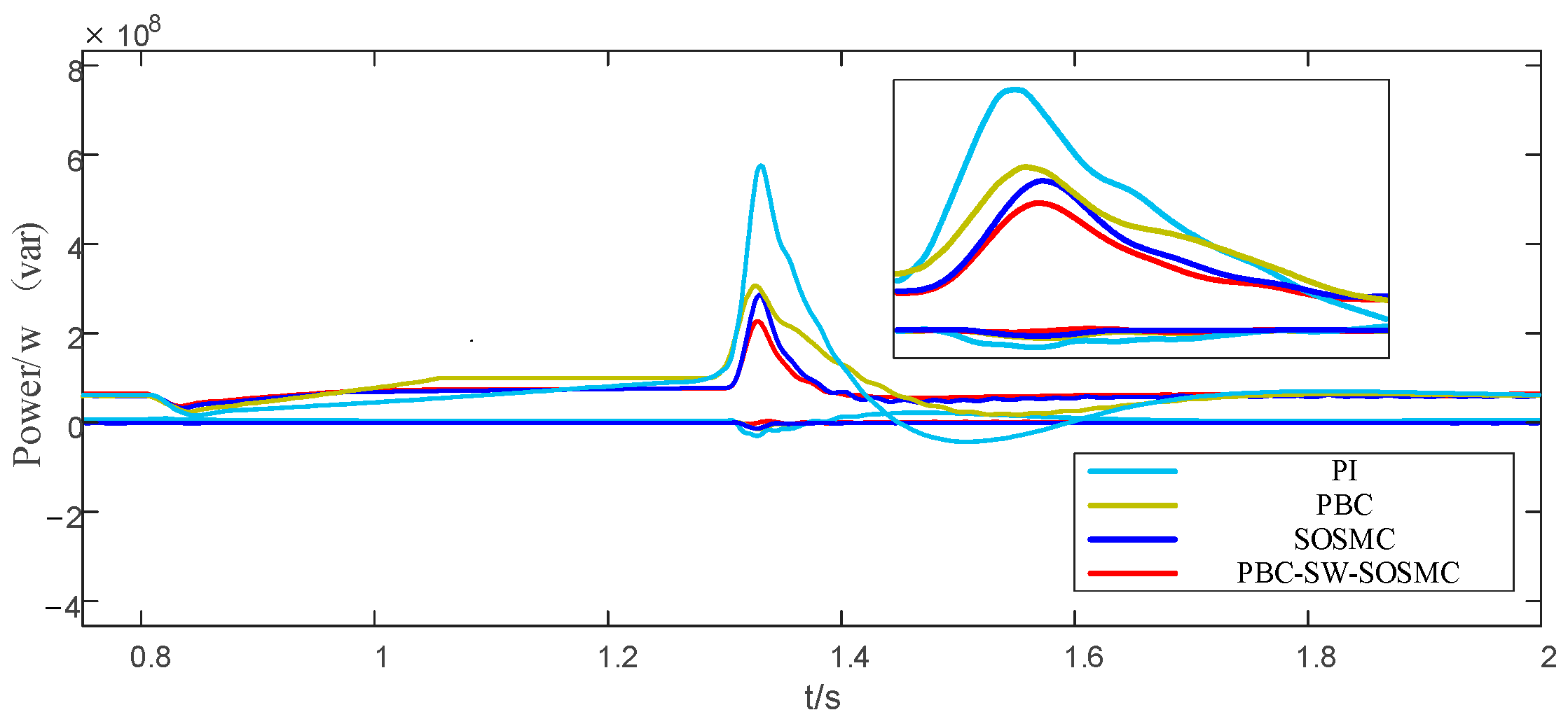
Figure 8 displays the simulated waveform of the MMC-PET grid-side power. As the load is resistive, the overall reactive power of the system remains constant at 0. It is evident from the figure that the grid-side active power is no longer stable during the load change period of 0.8–1.3 s under PI control. Moreover, the power curve overshoots more after the load is removed at 1.3 s and only stabilizes after 0.4 s. The use of PBC reduces the overshooting power curve compared to PI and maintains stability during the load mutation period. On the other hand, the power curve of SOSMC can maintain stability during the load change period and improve dynamic performance. After adopting PBC-SW-SOSMC, the power curve stabilizes in less than 0.2 s after the load change period. The power curve stabilizes smoothly and without buffeting, with minimal overshooting. After the load is removed, the power stabilizes more quickly, demonstrating the effectiveness of the control strategy proposed in this paper.

The DC current obtained after transforming the three-phase current into dq components can more intuitively compare the differences between the control effects. Therefore, we compared the d-axis components under the four control methods. Figure 9 shows the simulated waveform of the d-axis component of the MMC-PET grid-side current. During the load change period, the waveform recovery time of the d-axis component of the grid-side current is longer, and the overshoot is larger under PI control and PBC. The overall control effect of SOSMC is slightly better than that of the PI control and PBC, but there is still high-frequency buffeting. After adopting PBC-SW-SOSMC, the waveform overshoot is reduced, and the regulation time is shortened. This effectively suppresses the influence of sudden load changes on the gird side and results in a remarkable control effect.

Table 2. Dynamic performance indicators of the grid-side load change.

Control Strategy	Rising Time/s	Overshoot/%	Adjustment Time/s
PI	0.453	2.32	0.441
PBC	0.335	0.96	0.322
SOSMC	0.186	0.81	0.254
PBC-SW-SOSMC	0.172	0.44	0.167

compares detailed performance metrics.

5.2. Temporary Voltage Unbalance

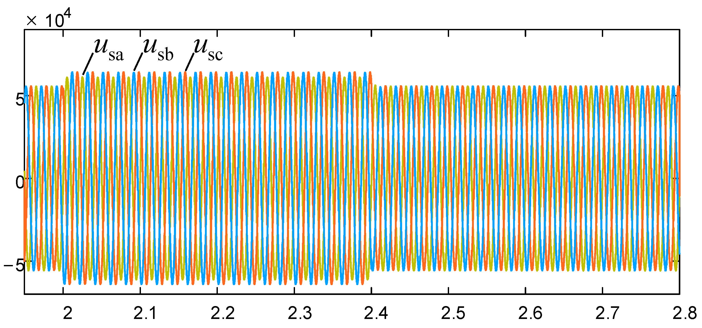
Voltage unbalance is a common issue in power grid operation, and it is important to maintain a balanced voltage to ensure efficient power grid operation. This paper aims to study the control effect of the system under the rise and fall in voltage unbalance. To achieve this, the voltage rise is set to rise between 2–2.4 s, lasting for 0.4 s. In phase A, the voltage rises by 10%, while in phases B and C, the voltage rises by 15%. At 2.4 s, the three-phase voltages drop to their initial value, as shown in Figure 10. The experimental results of the unbalanced temporary rise and fall in voltage on the input stage of the MMC-PET are presented in Figure 11, Figure 12 and Figure 13.

Figure 11 shows the simulated waveforms of the high DC side voltage of the MMC-PET when the unbalanced rise and fall in voltage in the grid occurs. Figure 11 displays that during the voltage rise and fall, the PI control tends to stabilize for a longer time, and the amount of overshoot is larger; the control effect of PBC is better than that of the PI control, and the overshoot is reduced, but the waveform is not smooth enough, and the recovery time is longer; the high DC side voltage under SOSMC has a small overshoot and faster response speed, and it can be restored to stability in a shorter time, but there is a buffeting in the period of 2–2.1 s of the waveform. PBC-SW-SOSMC also has the advantages of small overshoot and fast response speed; the waveform can be stabilized without buffeting after 0.05 s and the overall control effect is better.

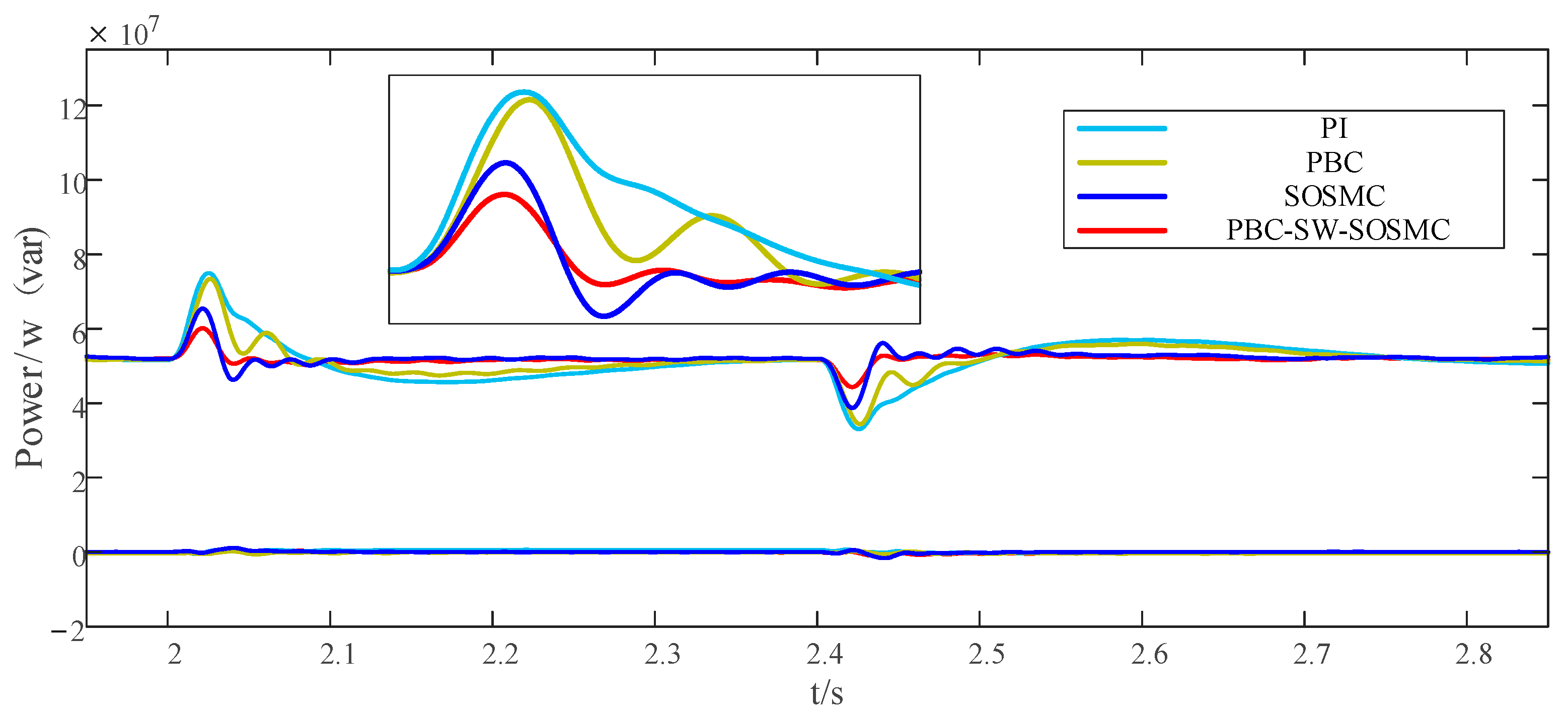
Figure 12 shows the simulation waveform of the grid-side power of MMC-PET when the unbalanced rise and fall in the grid voltage occurs. From Figure 12, it can be seen that when the grid voltage temporarily rises during 0.2–0.24 s, the grid-side power waveform under PI control can basically no longer be kept stable, and the overshoot is larger. At the same time, when the grid-side voltage drops to the initial voltage, it still takes 0.3 s to recover the stable state. Compared with the PI control and the PBC, the grid-side power waveform with SOSMC is improved, and it can be recovered to a stable state in a short period of time, but there are large fluctuations in the waveform. And the grid-side power waveform under PBC-SW-SOSMC not only has a shorter regulation time, but also has less overshoot, so it is obvious that the control effect of PBC-SW-SOSMC is more significant.

Figure 13 shows the simulated waveform of the d-axis component of the MMC-PET grid-side current when the unbalanced rise and fall in the voltage in the grid occurs. Under the PI control, the response speed of the d-axis component during the voltage rise is slow and the overshoot is large. PBC and SOSMC can restore the stability of the d-axis component in a short time, which improves the overall control effect compared with the PI control, but the overall fluctuation of the waveform is large, and the anti-jamming ability is poor. After adopting PBC-SW-SOSMC, the d-axis component can reach a new stable state within 0.05 s, and the overshoot is smaller, and the waveform is smoother. Obviously, PBC-SW-SOSMC can effectively inhibit the effect of voltage rise and fall on the system and has a stronger anti-interference capability.

Table 3. Dynamic performance indicators of the temporary voltage unbalance.

Control Strategy	Rising Time/s	Overshoot/%	Adjustment Time/s
PI	0.286	12.7	0.274
PBC	0.141	9.6	0.135
SOSMC	0.083	6.4	0.075
PBC-SW-SOSMC	0.045	2.1	0.041

compares detailed performance metrics.

Figure 14 shows the FFT analysis of the grid-side current. The harmonic content of the grid-side current under PI control is the highest, with a THD of 2.39%. Compared with PI control, the harmonic content of the grid-side current after PBC and SOSMC is relatively low, with THDs of 1.93% and 1.85%, respectively. PBC-SW-SOSMC has the lowest harmonic content, with a THD of 1.49%. PBC-SW-SOSMC can keep the power quality of the grid-side current at a high level with a better control effect.

5.3. Output Stage Load Connections

This condition is set to 3 s when the output stage is connected to a non-linear load. The experimental results on the input stage are shown in Figure 15.

The connection of nonlinear load at the output stage at 3 s causes the fluctuation of high DC, and the increase in load also increases the active power on the grid side, but it can return to the steady state under the action of the control loop on the grid side and bring it back to the vicinity of the reference value. From Figure 10, it can be seen that under PI control and passive control, the voltage and power can maintain the steady state and return to the reference value, but the corresponding speed is slower and there is a large overshoot value; under the second-order sliding mode control, the dynamic characteristics of the system have been improved; compared with the above control strategies, under the second-order sliding mode control of the passive super-helicopter, the system has the fastest response speed and the smallest overshoot value, which has certain advantages in the case of nonlinear load access. Advantages.

From Figure 15c, when a nonlinear load is added to the output stage, the value of the d-axis component of the grid-side current increases and reaches a new steady state with PI control and PBC. However, the regulation speed is slow. With SOSMC, the regulation speed significantly improves, but there is buffeting in the waveform during the transition to the new steady state. In comparison, PBC-SW-SOSMC offers the fastest regulation speed, the best dynamic performance, and effectively attenuates buffeting.

Table 4. Dynamic performance indicators of output stage load connections.

Control Strategy	Rising Time/s	Overshoot/%	Adjustment Time/s
PI	0.172	11.1	0.337
PBC	0.145	10.4	0.236
SOSMC	0.119	6.5	0.137
PBC-SW-SOSMC	0.094	4.6	0.101

compares detailed performance metrics.

Figure 16 displays the experimental simulation curves of the output stage. (a), (b), (c), and (d) show the three-phase voltages, the low-voltage DC side voltage, the current of the output stage, and the power of the output stage obtained from the output stage inverter, respectively. When the nonlinear load is connected, the controller of the input stage effectively controls the stability of the voltage on the high-voltage DC side. Although there may be fluctuations in the DC voltage, it remains stable due to the input equalization control of the intermediate stage. The inclusion of the nonlinear load results in an increase in the output current and a step change in the active and reactive power of the output stage. However, the regulation time is short and can be stabilized by the controller.

6. Conclusions

This paper focuses on the power electronic transformer of the modular multilevel converter (MMC-PET) and proposes a passive super-twisting second-order sliding mode control strategy. The strategy combines passivity-based control and super-twisting second-order sliding mode control and is compared to three other control strategies: PI control, passivity-based control, and second-order sliding mode control. The comparative analyses are conducted under different non-ideal working conditions. Simulation experiments lead to the following conclusions:

(1)

The use of passive super-twisting second-order sliding mode control can effectively suppress the DC side voltage, power, and current fluctuations of the MMC-PET under non-ideal operating conditions, thereby improving the reliability of the system operation.

(2)

The proposed passive super-twisting second-order sliding mode control strategy has been found to have stronger anti-interference ability, faster response speed, and greater robustness compared to PI control, passivity-based control, and second-order sliding mode control. This makes it more suitable for the transmission and distribution system of MMC-PET.

References

- Li, Z.X.; Gao, F.Q.; Zhao, C. Research review of power electronic transformer technologies. Proc. CSEE 2018, 38, 1274–1289. [Google Scholar]
- Sun, K.; Lu, S.L.; Yi, Z.Y. A review of high-power high-frequency transformer technology for power electronic transformer applications. Proc. CSEE 2021, 41, 8531–8545. [Google Scholar]
- Ma, D.; Chen, W.; Shu, L. A MMC-Based Multiport Power Electronic Transformer with Shared Medium-frequency Transformer. IEEE Trans. Circuits Syst. II Express Briefs 2020, 68, 727–731. [Google Scholar] [CrossRef]
- Zhu, L.; Li, C.S.; Lu, Y.P. Fault-tolerant Operation Technology for Three-level Cell Power Electronic Transformer. Autom. Electr. Power Syst. 2023, 47, 144–154. [Google Scholar]
- Xu, W.Y.; Zhen, C.H.; Xu, J.Z.; Zhao, C.Y. Average-value model of cascaded H-bridge type power electronic transformer. Electr. Power Autom. Equip. 2023, 43, 190–196. [Google Scholar]
- Lan, Z.; Tu, C.M.; Xiao, F. The power control of power electronic transformer in hybrid AC-DC microgrid. Trans. China Electrotech. Soc. 2015, 30, 50–57. [Google Scholar]
- Zheng, T.; Wang, K.; Zheng, Z.D.; Pang, J.P.; Li, Y.D. Review of Power Electronic Transformers Based on Modular Multilevel Converters. Proc. CSEE 2022, 42, 5630–5649. [Google Scholar]
- Zhou, Y.D.; Xu, Y.H.; Lv, X.H. Grounding Design and Fault Characteristic Analysis of MMC Based Power Electronic Transformer in Distribution Network. Power Syst. Technol. 2017, 41, 4077–4088. [Google Scholar]
- Zheng, T.; Guo, Y.F.; Lv, W.X.; Piao, Y. Protection for Low-voltage DC Distribution Network Based on Fault Ride-through Strategy of Power Electronic Transformer. Autom. Electr. Power Syst. 2023, 47, 152–161. [Google Scholar]
- Li, Y.X.; Li, Y.; Han, J.Y. A MMC-SST based power quality improvement method for the medium and high voltage distribution network. In Proceedings of the 16th International Conference on Environment and Electrical Engineering (EEEIC), Florence, Italy, 7–10 June 2016; IEEE: Piscataway, NJ, USA, 2016; pp. 2101–2106. [Google Scholar]
- Yuan, Y.S.; Tang, Z. Research on operation of power electronic transformer under voltage drop in intelligent distribution network. Power Autom. Equip. 2019, 39, 44–49. [Google Scholar]
- Khalid, Y.; Nor, Z.B.Y.; Vijanth, S.A. Development of power electronic distribution transformer based on adaptive PI controller. IEEE Access 2018, 6, 44970–44980. [Google Scholar]
- Fang, Y.; Xu, N.; Liu, Y. Hybrid Linear Predictive Control Scheme Based on PIR and MPC for MMC. In Proceedings of the 2023 IEEE 2nd International Power Electronics and Application Symposium (PEAS), Guangzhou, China, 10–13 November 2023; pp. 491–495. [Google Scholar]
- Wei, X.; Zhu, X.S.; Ge, J. Improved droop control strategy for parallel operation of cascaded power electronic transformers. High Volt. Technol. 2021, 47, 1274–1282. [Google Scholar]
- Zhang, C.; Jiang, Y.; Xing, X.; Li, X.; Qin, C.; Zhang, B. Passivity-Based Control Method for Three-Level Photovoltaic Inverter to Mitigate Common-Mode Resonant Current. IEEE Trans. Ind. Inform. 2023, 19, 9733–9744. [Google Scholar] [CrossRef]
- Bao, K.Q.; Wu, H.H.; Cheng, Q.M. Passive based control strategy of electric springs based on E-L model. High Volt. Eng. 2021, 1, 1–10. [Google Scholar]
- Xie, Z.K.; Yang, J.M.; Huang, W. Passive control of Archimedes wave swing wave power generation system. Control. Theory Appl. 2019, 36, 383–388. [Google Scholar]
- Cheng, Q.M.; Sun, W.S.; Cheng, Y.M. Passive control strategy of MMC under power grid voltage imbalance. Power Autom. Equip. 2019, 39, 78–85. [Google Scholar]
- Cheng, Q.M.; Fu, W.Q.; Xie, Y.Q.; Zhou, Y.T.; Ye, P.L. Research on Passivity-Based Control Drive System of Permanent Magnet Synchronous Motor Based on MMC-PET. South. Power Syst. Technol. 2022, 16, 83–91. [Google Scholar]
- Liu, Z. Fixed-Time Sliding Mode Control for DC/DC Buck Converters with Mismatched Uncertainties. IEEE Trans. Circuits Syst. 2023, 70, 472–480. [Google Scholar] [CrossRef]
- Shi, S.; Zhang, G.S.; Min, H.F. Prescribed-time SOSM control of nonlinear systems subject to mismatched terms. Control. Decis. 2023, 8, 1–9. [Google Scholar]
- Ma, F.J.; Zhu, Z.; Min, J. Model analysis and sliding mode current controller for multilevel railway power conditioner under the V/v traction system. IEEE Trans. Power Electron. 2019, 34, 1243–1253. [Google Scholar] [CrossRef]
- Guo, J. The Load Frequency Control by Adaptive High Order Sliding Mode Control Strategy. IEEE Access 2022, 10, 25392–25399. [Google Scholar] [CrossRef]
- Swikir, A.; Utkin, V. Chattering analysis of conventional and super twisting sliding mode control algorithm. In Proceedings of the 2016 14th International Workshop on Variable Structure Systems. Nanjing, China, 1–4 June 2016; IEEE: Piscataway, NJ, USA, 2016; pp. 98–102. [Google Scholar]
- Zhou, J. Decentralized Robust Control for Vehicle Platooning Subject to Uncertain Disturbances via Super-Twisting Second-Order Sliding-Mode Observer Technique. IEEE Trans. Veh. Technol. 2022, 71, 7186–7201. [Google Scholar] [CrossRef]
Figure 1.
Overall Structure of MMC-PET.