
A Multi-Source Braking Force Control Method for Electric Vehicles Considering Energy Economy

College of Automotive Engineering, Jilin University, Changchun 130025, China
*
Author to whom correspondence should be addressed.
Energies 2024, 17(9), 2032; https://0-doi-org.brum.beds.ac.uk/10.3390/en17092032
Submission received: 28 February 2024
/
Revised: 31 March 2024
/
Accepted: 16 April 2024
/
Published: 25 April 2024
(This article belongs to the Special Issue Energy Management Control of Hybrid Electric Vehicles)
Abstract
:Advancements in electric vehicle technology have promoted the development trend of smart and low-carbon environmental protection. The design and optimization of electric vehicle braking systems faces multiple challenges, including the reasonable allocation and control of braking torque to improve energy economy and braking performance. In this paper, a multi-source braking force system and its control strategy are proposed with the aim of enhancing braking strength, safety, and energy economy during the braking process. Firstly, an ENMPC (explicit nonlinear model predictive control)-based braking force control strategy is proposed to replace the traditional ABS strategy in order to improve braking strength and safety while providing a foundation for the participation of the drive motor in ABS (anti-lock braking system) regulation. Secondly, a grey wolf algorithm is used to rationally allocate mechanical and electrical braking forces, with power consumption as the fitness function, to obtain the optimal allocation method and provide potential for EMB (electro–mechanical brake) optimization. Finally, simulation tests verify that the proposed method can improve braking strength, safety, and energy economy for different road conditions, and compared to other methods, it shows good performance.
1. Introduction
With the development of science and technology, smart and low-carbon environmental protection have become the mainstream trend of future automobile development. Electric vehicles are the ideal platform for developing smart automobiles and have attracted much attention and research due to their clean, efficient, and energy-saving characteristics. An EMB does not use the original hydraulic and pneumatic systems but uses a motor as the braking source to achieve high precision in brake force control. However, due to the highly nonlinear nature of vehicle dynamics, the design and optimization of electric vehicle brake systems still faces multiple challenges, such as coordination between the power domain and the chassis domain and the trade-off between safety and economy. How to reasonably allocate and control brake torque to improve the energy efficiency and braking performance of electric vehicles is one of the core issues [1,2].
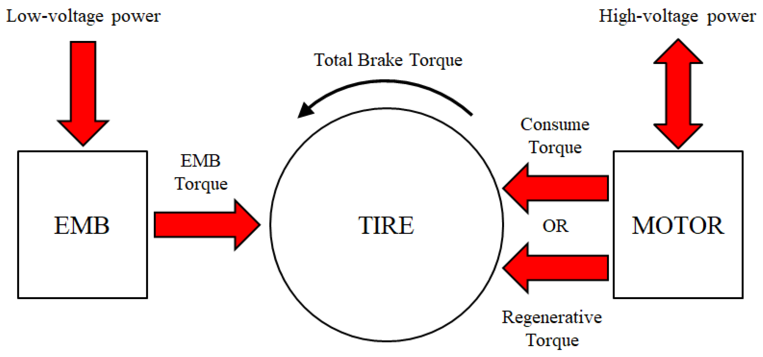
For an EMB, the main drawbacks are large mass and volume, which have negative effects on reducing mass, assembly, and layout. Reducing the volume of an EMB system is usually achieved by changing its internal structure, such as by using a cam configuration and a wedge-type self-increasing force configuration. The cam configuration has less axial space utilization and has a compact structure, but the cam and support are disconnected by points or lines, which are prone to wear [3,4]. The wedge-type self-increasing force configuration can greatly reduce the required driving power and the volume of the actuator, but it is difficult to control due to factors such as wear and temperature [5,6]. The above solutions can ensure that the EMB can provide sufficient braking intensity while reducing the volume, but it is still difficult to reduce the volume of EMB systems to the size of traditional brakes, and they will still face problems such as excessive lower mass and difficulty with assembly and layout. In order to solve the problem of the large volume of EMB systems, for electric vehicles, using the energy recovery of the driving motor or power-consuming braking to share a part of the braking force that should be provided by an EMB has become an effective solution. If the motor provides a larger brake torque, the EMB will provide a smaller brake torque. As shown in Figure 1, in the braking system of electric vehicles, there are three sources of braking force: 1. EMB braking, 2. driving motor energy recovery, and 3. driving motor power-consuming braking. The allocation scheme of the braking source can be roughly divided into three types based on: vehicle dynamics, fuzzy control, and intelligent algorithms. As for those based on vehicle dynamics, some researchers have proposed to develop different braking force distribution strategies according to different braking conditions to improve vehicle stability and braking efficiency, but this method does not consider the response characteristics of switching between different braking sources [7]. Some researchers have proposed a decision-making method based on energy recovery demand for energy efficiency considerations: this method formulates different strategies according to the charging state and energy recovery demand of the battery, but this method takes more consideration of energy recovery efficiency and less consideration of overall performance [8]. Some researchers have proposed a decision-making method based on predictive control to plan the distribution of vehicle braking power sources in advance to reduce the impact of the response characteristics of each system on vehicle performance. However, this method is too idealistic and is difficult to achieve under complex road conditions and scenarios [9,10,11]. Fuzzy control refers to using a fuzzy controller to determine the size of the motor braking torque based on the vehicle’s driving state and expert experience, and then it combines the formulated front and rear axle braking force distribution strategy to obtain the braking force distribution strategy. Fuzzy control has good robustness and is easy to implement, but its formulation depends on experience and parameter calibration, which requires a lot of manual cost [12,13]. Intelligent algorithms include neural network control and particle swarm optimization algorithm control. Neural network control refers to controlling the regenerative braking torque based on the braking force distribution combined with neural network algorithms to improve the efficiency of braking energy recovery. Neural network control has high classification accuracy and strong parallel processing capabilities, but it requires a large number of training samples, and the data collection and preprocessing process requires a lot of computing resources and costs [14,15]. A particle swarm optimization algorithm refers to using the theory of particle swarm algorithms to optimally distribute the braking force in the regenerative braking process and has high braking energy recovery efficiency. A particle swarm optimization algorithm has fast search speed and can achieve multi-objective optimization, but its optimization goal is achieved through iterative methods, which will result in poor real-time computing capabilities [16]. The adaptability and convergence speed of the above methods are poor, so it is necessary to optimize the adaptability of braking force allocation strategies.
In addition, there are also coordination methods between the ABS and the regenerative braking system (RBS) or the power-consuming braking of the driving motor, which makes it difficult for the driving motor and the mechanical brake to work together to meet the high-frequency torque fluctuation requirements of ABS control. The role of ABS is to make the vehicle maintain sufficient maneuverability and stability under high braking conditions so as to improve road safety, and in the case of poor road adhesion conditions, the demands on the system are greater [17,18]. ABS initially uses a rule-based algorithm that takes into account slip rate and wheel deceleration. These methods do not have the capability of continuous feedback control, and while such methods are robust for the vehicle’s possible operating conditions, they provide only sub-optimal performance for wheel slip rate tracking control. As a result, incremental improvements have followed at the expense of increasing the complexity of tuning [19], such as algorithms for estimating maximum transmitted torque or torque control [20]. Some scholars have proposed slip controllers [21], but the essence remains unchanged. Subsequently, there has been growing interest in model-based state feedback controllers, especially MPC. Some researchers have proposed linear MPC to discuss longitudinal slip tracking performance during transitions from high-adhesion to low-adhesion surfaces [22], and others have compared MPC strategies to PID controllers and evaluated them on electric vehicle prototypes [9]. In the study of MPC algorithms for ABS, some scholars have discussed the anti-lock control of internal-combustion-engine-driven vehicles and have compared four-linear-MPC strategies with hybrid-explicit MPC, and the performance of the hybrid strategy is comparable to that of a well-tuned PID controller [23]. At the same time, some researchers have shown that the implementation time step has a greater impact on the anti-lock performance of electric vehicles than the selected control technology [24]. To sum up, more efficient ABS requires a controller with higher tracking performance and less computation time. In order to solve the coordination problem between RBS and ABS, there are currently three approaches: using only mechanical braking force for ABS control, using only electric braking force for ABS control, and combining mechanical and electric braking forces for ABS control. For the first approach, this ensures driving safety, but it completely wastes the braking force of the motor, making the idea of using the driving motor to share part of the braking demand for an EMB a fantasy, and it also affects the energy economy during the braking process [25,26,27]. For the second approach, due to the limitations of motor battery characteristics and matching, the electric braking torque may not be able to meet the braking demand, resulting in insufficient braking force during high-intensity braking in actual vehicle driving, which affects braking safety. This method only exists in idealized simulation verification [28,29,30]. For the third approach, the main control methods can be divided into the following categories: model-following control, logic threshold value method, and fuzzy control. In the model-following control method, the electric braking force is responsible for the high-frequency part of the braking demand, and the mechanical braking force is responsible for the low-frequency part of the braking demand. A combination of a PQ-method, a filter-based frequency band selection method, and a model-following control method is used to control the two braking forces to achieve ABS function. The PQ-method is one of the “Parallel Control” methods that considers different response characteristic. It is simple and effective, but it still cannot fully utilize the motor’s capabilities [31]. The logic threshold value method is an optimal-slip-rate-based compensation control strategy, which uses an optimum control method to determine the optimal braking torque of the wheels, uses the logic threshold value method to control the frictional braking force, and uses the motor torque to compensate for the difference between the optimal braking torque and the frictional braking torque. This method has good robustness, accuracy, and effectiveness and is less affected by noise, but it still cannot fully utilize the motor’s capabilities [32]. Fuzzy control is based on the vehicle’s driving state and expert experience and uses a fuzzy controller to determine the size of the motor and mechanical braking forces. Fuzzy control has good robustness, is easy to implement, and has a good chance of utilizing the motor’s energy recovery capabilities, but its reliance on experience and parameter calibration requires a lot of manual cost [33,34]. In addition, its transient response to braking torque is poor, making it highly susceptible to noise and difficult to control under complex conditions. In summary, the third approach mentioned above can ensure that the braking torque meets the control requirements and can also utilize the motor’s energy recovery capabilities to some extent. However, in order to fully utilize the motor’s capabilities, precise control and stable braking torque decisions are needed, as these provide a foundation for coordinating control between the driving motor and EMB. For the EMB system, the ABS function can be replaced by a slip rate controller, which precisely controls the braking torque to maintain a stable slip rate throughout the entire braking process, increasing braking comfort and improving energy recovery efficiency. In summary, the decision about braking force demand is extremely important, and stable braking force demand can provide the potential to fully utilize the motor’s capabilities.
In this paper, a multi-source braking force system and its control strategy is proposed with the aim of improving the braking force, safety, and energy efficiency during the braking process. In the proposed strategy, firstly, a vehicle–road state observer based on vehicle dynamics is developed to meet the requirements of subsequent control [35,36,37]. Secondly, a braking force control strategy based on ENMPC is developed to replace traditional ABS strategies. By using closed-loop slip rate control, stable demand for braking force is achieved to fully utilize the motor’s capabilities [38,39,40]. Thirdly, in order to ensure that the motor’s capabilities can be used to share part of the braking force for an EMB, the entire electric braking system is optimized based on the motor battery’s characteristics. Finally, a reasonable allocation of braking sources is achieved through the grey wolf algorithm, using energy consumption as the fitness function to obtain the optimal allocation method, which improves energy efficiency and provides the possibility of reducing the size of the EMB system [41,42]. The innovations of this paper are as follows:
- The feasibility of using the motor’s energy recovery or power-consuming braking to share part of the braking force for an EMB is theoretically elaborated based on the analysis of motor battery characteristics. This aims to reduce the braking force demand of the EMB system and its size.
- In order to ensure that the braking torque can be easily adjusted using the driving motor, a slip rate controller is designed based on the ENMPC algorithm, which makes the demand torque more stable compared to traditional ABS, thereby improving braking performance.
- In order to achieve a reasonable allocation of the three braking forces, a braking source allocation strategy is developed based on the grey wolf algorithm, which improves the fitness of the braking source allocation and the overall energy efficiency of the vehicle.
2. Vehicle and Component Model
In this paper, an electric box-type truck is the focus, and the corresponding configuration is illustrated as Figure 2. The studied vehicle comprises a single drive motor for the rear axle, a power battery, a gearbox, and a main reducer. The electronic mechanical brake (EMB) acts as the brake system actuator and is controlled by the brake control unit. The brake control unit communicates via the controller area network (CAN) bus, which connects it to the electronic mechanical brake motor control unit and the vehicle control unit. Additionally, the vehicle is equipped with regenerative braking functionality. Under conditions conducive to energy recovery, the drive motor operates as a generator, producing power to recharge the battery. During this phase, the drive motor can supply braking torque, facilitating vehicle deceleration.
The vehicle parameters are shown in Table 1.
2.1. Vehicle Mathematical Model
During vehicle operation, the power sources should provide tractive force that overcomes the resistance of the vehicle in order to drive the studied vehicle. The various resistances include air resistance, slope resistance, and acceleration resistance, and the corresponding relationship between the tractive force and the resistance is formulated as:
where m denotes the vehicle mass, v denotes the vehicle longitudinal velocity, denotes the motor torque, denotes the transmission efficiency, r denotes the wheel rolling radius, denotes the air resistance coefficient, A denotes the windward area, denotes the air density, f denotes the road rolling resistance co-efficient, denotes the road grade, denotes the rotary mass coefficient, denotes the rotating inertia of the wheels, denotes the rotating inertia of the motor, denotes the main reduction gear ratio, and denotes the vehicle’s transmission ratio.
2.2. EMB Actuator Response Characteristics
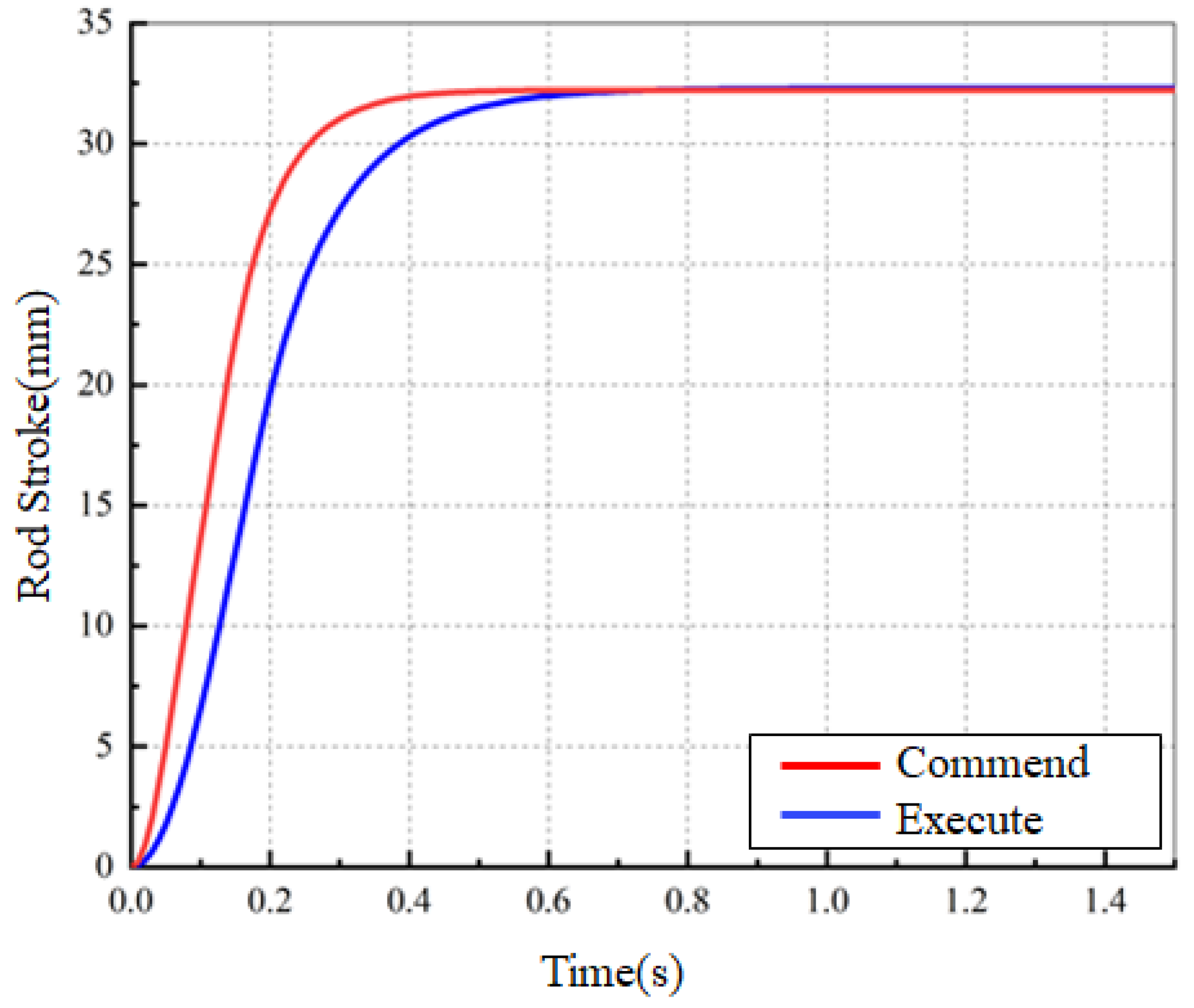
An electro–mechanical brake (EMB) realizes brake control by means of a motor-driven transmission mechanism and a clamping brake disc, thus realizing decoupling of the brake pedal and the brake torque at the mechanical level. Meanwhile, an EMB has the advantages of fast response, high control accuracy and low maintenance cost compared with pneumatic brake systems. The response characteristic of an EMB are shown in Figure 3.
2.3. Tire Model
The fitting of a magic formula is based on test data, and its fitting accuracy is high, but the calculation is large, so it is more suitable for product design, automobile dynamic simulation, test comparison, and other fields that require accurate descriptions of tire mechanical properties [43]. Thus, the magic formula is utilized in this paper to calculate the tire force:
In the equation, Y represents lateral force, longitudinal force, or self-aligning torque, X signifies slip angle or longitudinal slip ratio, denotes the peak factor, stands for the stiffness factor, represents the curvature factor, signifies the curvature factor, represents lateral curve shift, and represents vertical curve shift.
The primary focus of this study is the influence of the longitudinal slip ratio on tire forces. The formula for calculating the slip ratio is as follows:
where represents the radius of the tire, represents the speed of the tire, and represents the linear speed of the tire. When the vehicle travels in a straight line, .
2.4. Drive Motor Model
The electric braking torque of the energy regeneration system is provided by the motor. The external characteristics and the efficiency of the motor are depicted as Figure 4.
Based on Figure 4, the motor efficiency can be determined by the motor speed and motor torque, which can be shown as: Equation (4). The formula for calculating the motor output power is:
where represents the speed of the motor, and represents the output torque of the motor.
In this paper, only the motor serving as a load to the battery is considered. The battery output power can be expressed as:
where represents the battery load current, and signifies the terminal voltage of the battery.
During battery discharge, the battery output power is positive, indicating energy transfer from the battery to the motor. Conversely, during battery charging, the battery output power is negative, indicating energy transfer from the motor to the battery. Hence, the power of the motor and the battery is shown as:
During the modeling phase, the motor torque can be approximated as a first-order response, and according to the simulation step size , the motor’s required torque is shown as:
During energy regeneration braking involving the motor, the torque is transmitted through the gearbox, driveshaft, main reducer, and half-shafts to the driving wheels. The electric braking torque acting on the driving wheels is shown as:
where represents the gearbox ratio, and signifies the main reducer ratio.
2.5. Battery Model
A second-order RC circuit battery model was constructed with an initial battery capacity of 318 Ah. The battery’s state of charge (SOC) and terminal voltage concerning the load current are expressed as:
where represents the current of the motor, represents the voltage of a first-order RC circuit, represents the voltage of a second-order RC circuit, denotes the number of parallel battery modules, represents the number of series-connected battery modules, stands for the electromotive force of the power source, and and correspond to the first-order RC circuit resistance and capacitance, respectively. Additionally, and indicate the second-order RC circuit resistance and capacitance, respectively. Values for , , , , and are obtained using the approach described in Equation (11), utilizing battery SOC and temperature to access the table.
3. Multi-Source Braking Force System and the Control Strategy
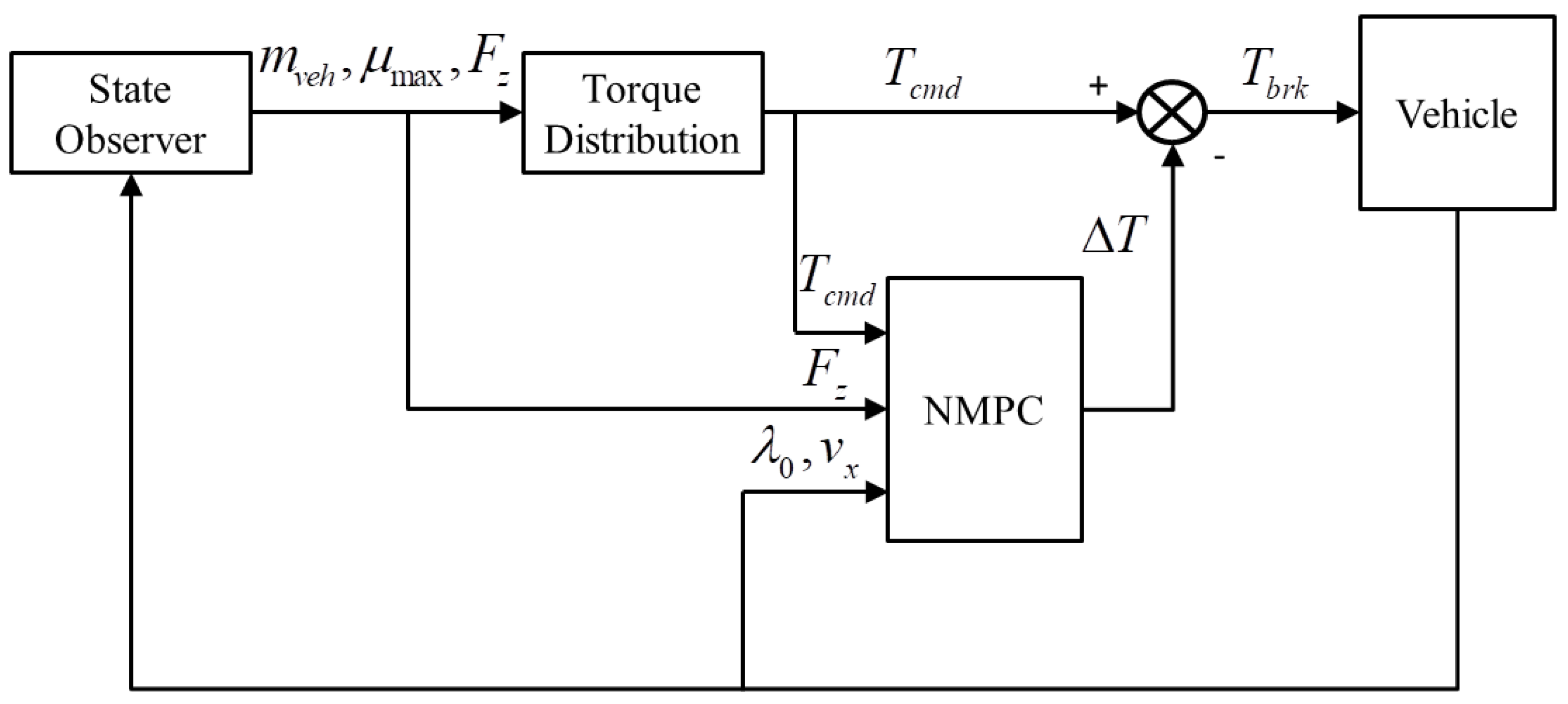
In this section, a discussion of the structural refinement of the braking system is initiated, wherein the energy-consuming braking of the drive motor is deliberated as a supplementary source of braking force. This approach aims to decrease the performance demands on the electro–mechanical brake (EMB) motor and to achieve downsizing. Concerning the control strategy, a vehicle motion state observation system is established. Through the outcomes of state observation, computation of the required braking torque for the vehicle is performed, along with the provision of a reference wheel slip ratio concurrent with the allocation of the required braking torque. The allocation is bifurcated into two steps. Initially, based on the outcomes of state observation, the braking torque is distributed to individual wheels. Subsequently, for the driving wheels, the allocated braking force undergoes mechanical braking (EMB braking), energy recovery braking, and distribution of torque from the power-consuming action of the drive motor. This ultimately enables control of the vehicle’s braking torque and the regression of the actual wheel slip ratio to the targeted slip ratio. The overall architecture of the control strategy is depicted in Figure 5.
3.1. Enhancements to the Configuration of Multi-Source Braking Power System
In order to solve the problem of the large volume of EMB systems, for electric vehicles, using the energy recovery of the driving motor or power-consuming braking to share part of the braking force that should be provided by the EMB has become an effective solution. If the motor provides larger brake torque, the EMB will provide a smaller brake torque.
The recovery motor torque can be increased by increasing the output voltage of the motor, but the battery cannot accept excessive voltage from the motor. A series resistor needs to be added, with the aim of diverting a portion of the motor output voltage so that the battery can accept it.
The motor’s external characteristics curve as installed in the target vehicle is illustrated in Figure 6. The higher the motor speed, the smaller the torque generated. Therefore, when utilizing the braking capability of the drive motor, it is essential to consider the most extreme scenario: whether at maximum motor speed , the required deceleration for the vehicle can be achieved.
During the braking process, if we solely consider the drive motor’s effect on the vehicle within the constant power region of the motor’s external characteristics curve, we have:
where is the required power during vehicle braking, is the motor power for energy recovery when formulating, is the motor power during electric motor power consumption braking, and and are the efficiency of the transmission system.
The calculation of the maximum required braking power at the rear axle is shown as:
where is the maximum design speed of the vehicle, and is the rear axle load.
Based on the vehicle’s drivetrain system structure, Equation (14) represents the maximum design speed of the vehicle.
where represents the max gear ratio of the transmission.
In this scenario, to achieve the desired deceleration , the minimum counter electromotive force that the drive motor needs to generate can be represented as:
where is the rated motor current.
To ensure charging of the battery at the rated power, a series resistor is needed; the resistance value can be represented as:
where is the maximum charging power of the battery, and is the maximum internal resistance of the battery.
To reduce the EMB’s volume, the relationship between the EMB force required and the volume needs to be researched.
The mass and volume of the EMB primarily consist of the motor and rotating components. The volume of the transmission mechanism scales in proportion to the load it carries. For the motor, when maintaining its current and voltage as constant, the maximum output torque is directly proportional to the magnetic flux. Without altering the magnetic characteristics of the permanent magnet, the magnetic flux is directly proportional to the number of coil turns, denoted as “n”. The quantity of coil turns impacts the motor’s volume. This discussion solely considers the number of coil turns as a measure of the motor’s size, thereby establishing a direct correlation between the motor’s volume and the number of coil turns.
Based on the above analysis, we can infer that the maximum output torque of the motor is directly proportional to its volume, and simultaneously, the maximum torque output of the motor is directly proportional to the maximum deceleration it can produce.
The proportion by which the volume of the EMB motor decreases can be expressed as Equation (17) once the performance of the drive motor is established.
where is the maximum designed deceleration of the vehicle.
The required driving motor voltage at this point is shown as:
The resistance values of the fixed resistors to be connected in series are shown as:
3.2. Control Strategies for Multi-Source Braking Power System
3.2.1. Vehicle State Observer
A. Estimation of Vehicle Weight and Road Gradient:
Commercial vehicles serve a primary purpose of transporting passengers and goods. There is a substantial disparity in vehicle weight between empty and fully loaded states. Vehicle mass can differ by as much as 400% based on varying loads. Although the quality of the vehicle will not change during the driving process, the load will change greatly after loading and unloading, and a fixed set of parameters cannot meet the needs of vehicle control. Accurately estimating vehicle mass holds significant importance for enhancing control precision.
This study utilizes a recursive least squares method with a forgetting factor for parameter estimation, transforming Equation (1) into the standard expression of the least squares method, as shown in Equations (20)–(24).
where
After the controller is powered off, in order to ensure safety, the initial value of the mass estimation result is reset to the full load mass to ensure that the braking torque meets the requirements after the vehicle is powered on again.
B. Estimation of Tire–Road Adhesion Coefficient:
To meet the requirements of subsequent control strategies, the tire–road adhesion coefficient needs to be estimated.
The estimation method based on the (adhesion coefficient–slip ratio) model is a typical effect-based estimation approach that has seen extensive application in the field of automotive dynamics.
When the slip ratio is less than 0.07, it can be approximated that there exists a linear relationship between the adhesion coefficient and the slip ratio. Therefore, the road surface adhesion coefficient can be shown by Equations (25) and (26).
In Equations (25) and (26), k represents the slope of the “” curve, where and denote the longitudinal and vertical forces, respectively, acting on the tire at the current slip ratio . The term stands for the maximum tire slip ratio within the linear region and is set as . The variable p signifies the coefficient between the maximum adhesion coefficient in the linear region and the peak adhesion coefficient of the road surface and typically ranges from 1.2 to 1.4.
For the road adhesion coefficient at large wheel slip rates (), the magic tire model is represented as Equation (2); the detailed coefficient is represented as:
, , and have nothing to do with road adhesion, but is related to road adhesion:
where represents the coefficient related to road adhesion; the magic formula is matched under conditions of 0.8 road adhesion:
where represents the road adhesion, so that
The magic tire model can be written in the following nonlinear format:
with
where is the expression of the magic tire model, and is the noise during the measurement.
Define the variable as:
then we have
The form obtained by simplification meets the requirements of least squares parameter estimation, and the tire–road adhesion coefficient can be effectively estimated by the least squares method.
C. Estimation of Vertical Dynamic Load on the Wheels:
Based on the estimated mass and considering the axle load transfer due to longitudinal and lateral accelerations, vertical tire forces are calculated. The longitudinal axle load transfer caused by longitudinal acceleration is shown as Equations (37) and (38).
Similarly, considering the longitudinal axle load transfer caused by lateral acceleration, taking the front axle as an example, it is shown as:
Rearranging Equations (37)–(39), the dynamic vertical load on the vehicle’s left front wheel is shown as:
Similarly, the expressions for the dynamic vertical loads on the other wheels are given as shown in Equations (41)–(43).
where , , , and represent the vertical loads on the four wheels, and denote the longitudinal and lateral accelerations, respectively, a and b represent the longitudinal distances from the center of mass to the front and rear axles, respectively, and represents the height of the center of mass.
3.2.2. Calculation and Allocation of Required Braking Torque
In this section, based on driver and external braking requirements, the total vehicle mass and peak road adhesion coefficient are used to calculate the required braking torque for the entire vehicle. Then, based on the dynamic loads on each wheel, the required braking torque for each wheel is computed.
The aim of this study is to adjust the braking torque to maintain the slip ratio around the target value instead of the traditional ABS control strategy. An ENMPC is proposed to control the brake force, with the aim of keeping the slip ratio stable.
The relationship between braking torque and deceleration on a road surface with a specific adhesion is depicted in Figure 7. Excess braking torque not only fails to enhance deceleration but also increases tire slip, raising the probability of ABS activation and wheel lockup. Therefore, represents the minimum braking torque achievable on the current road surface to attain the maximum achievable deceleration.
As shown in Figure 8, the maximum achievable deceleration of a vehicle and the minimum braking force corresponding to this maximum deceleration vary across different road surface adhesions. On surfaces with lower adhesion coefficients, applying a smaller braking torque is adequate to reach the maximum braking potential the ground can offer. Therefore, if the road surface adhesion coefficient is known, real-time adjustments to the braking torque can be made based on this coefficient. This ensures that the braking torque does not exceed the corresponding value associated with the current road surface adhesion, significantly reducing the probability of ABS activation.
For commercial vehicles, the maximum achievable braking deceleration during braking processes is approximately . Normalizing the driver’s pedal displacement, denoted as , the demanded braking deceleration by the driver can be expressed as:
Considering the potential deceleration demanded from intelligent driver assistance systems, the overall vehicle’s required deceleration can be consolidated as:
At the vehicle level, the sum of the required longitudinal tire forces for the desired deceleration can be expressed as:
The relationship between the total torque acting on each wheel and the angular acceleration is as follows:
where is the longitudinal rotational inertia of the tire, represents the angular velocity of the tire, stands for the effective radius of the tire, denotes the driving torque, and represents the braking torque.
During braking, , ; also, the maximum deceleration the vehicle can achieve at a peak road adhesion coefficient is . Therefore, the vehicle’s overall required braking torque can be expressed as
According to the estimated results of , the braking torque for each wheel is:
where represents the theoretical braking torque required under the current braking intensity demand, while under emergency braking, adjustments should be made to to prevent wheel lockup.
3.2.3. Distributed Braking Torque Control Strategy
Due to vibrations and impacts experienced by vehicles during operation, sensors may suffer from errors and noise that affect the precision of parameter estimation. Therefore, it is necessary to make adjustments to the theoretical braking torque to ensure braking safety.
Hence, a compensatory braking torque is introduced based on the current slip ratio of each wheel:
Applying the adjusted target braking torque to each wheel ensures that the slip ratio remains within the desired range, significantly reducing the probability of ABS activation. Simultaneously, to ensure the motor can fully respond to the electric braking torque, it is crucial to maintain in a state of low-frequency minor fluctuations.
Differentiating the formula for the slip ratio yields:
Based on the previously derived brake force distribution and assuming equal utilization of the coefficient of adhesion by each wheel, we can conclude:
According to Equation (47), it can be deduced that:
Substituting Equations (52) and (53) into Equation (51), we get:
According to Equation (50), modify the required braking torque .
In the equation, represents the compensatory braking torque.
Use the current slip ratio and simulation time step to calculate the next time step slip ratio .
Given the known vehicle driver’s overall demanded deceleration, it is possible to calculate the required longitudinal force.
According to Equation (57), when the driver’s demand is determined, it is possible to calculate the slip ratio corresponding to the linear range, denoted as . The method for calculating the reference slip ratio, denoted as , is as follows:
The relationship between the braking torque and the slip ratio exhibits high nonlinearity. To address this highly nonlinear issue, model predictive control (MPC) is introduced. Based on the current operating conditions, MPC employs the predicted range of braking torque as a control parameter and predicts and observes the slip ratio within this predictive interval. The goal is to approach the desired slip ratio through prediction and then deduce the necessary braking torque to be applied within the predicted interval. This method is applicable across various conditions and demonstrates precise and effective control while possessing robustness. The model predictive control logic utilized in this paper is illustrated in Figure 9.
Consider the following discrete nonlinear system:
where represents the system state at time , denotes the system control at time , and signifies the system state at time .
Taking the slip ratio as the system state and the compensatory braking torque as the system control, applying control within the prediction horizon allows observation of the system state .
Taking the current control input as the compensatory braking torque and the currently observed variable as the slip ratio , then:
According to the magic formula:
The first-order Taylor expansion of Equation (60) at time yields:
Let ,
Incorporating Equations (61)–(63) into Equation (66) gives
Taking the predicted time t, we can obtain:
Iterate on Equation (68).
Equation (69) represents the relationship between the state variables at time t and the control variables at different time points. Similarly, the relationship between the state variables at each time point and the control variables at various time points can be derived, as shown in Equation (70).
Let , ,
,
Then, Equation (70) can be simplified:
During the braking process, it is necessary to control the actual slip ratio to be close to the reference slip ratio . This means that the difference between the actual and reference slip ratios should be as small as possible. Simultaneously, to prevent the system from being overly sensitive and to avoid large fluctuations in the braking torque, the compensatory braking torque should not be too large. Based on the reference slip ratio, let , where is a matrix with t + 1 rows and 1 column.
We introduce a cost function:
where ,
Let . Rearranging Equation (72), we obtain
In Equation (73), a smaller cost function better aligns with expectations. Matrices Q and R act as weight matrices, signifying the impact of each time step within the prediction horizon on control effectiveness and determining the importance between reducing the disparity of state variables from target states and minimizing control effort. It is essential to note that since the cost function is dimensionless, the values in matrices Q and R are influenced by the magnitudes of the state variables and control inputs. Smaller magnitudes should receive relatively larger weighting values.
In the cost function applied in this context, a higher value in matrix Q leads to a quicker convergence of the current slip ratio toward the target slip ratio. However, this can result in significant fluctuations in both braking torque and slip ratio to expedite the convergence of the slip ratio, subsequently increasing the probability of wheel lockup due to highly fluctuating slip ratios. Moreover, substantial fluctuations in braking torque can be disadvantageous for energy recovery in the motor system. Conversely, a higher value in matrix R may cause the compensatory braking torque to be too small. This scenario, especially during emergency braking on low-adhesion surfaces, slows down the convergence of the slip ratio and similarly raises the probability of wheel lockup.
Through the QP solver, the cost function is solved, and according to Equation (73), the value of the matrix U is solved when the cost function is minimized, , and is taken as the current control quantity to be applied, and the same computation is performed in each simulation step to obtain the control quantity at each moment.
3.2.4. Explicit Control Strategy
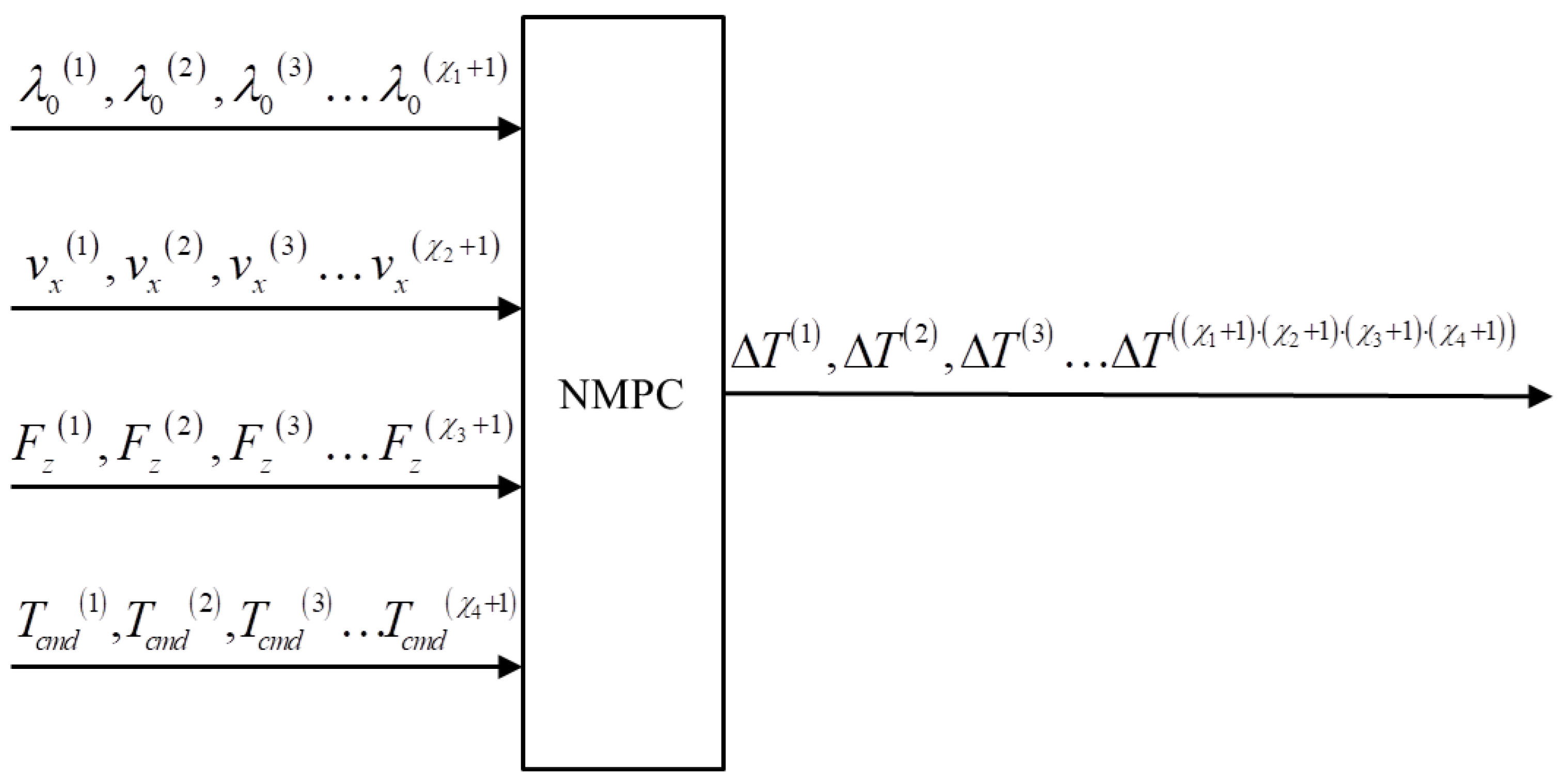
Due to the considerable computational load of model predictive control (MPC), its current focus remains on simulation testing, as the high computational load poses challenges to real vehicle testing. To expedite simulation speed and pave the way for practical vehicle trials, an approach integrating offline simulation with online solving has been proposed. This method replaces the implicit MPC solving process with an explicit one. By feeding the current vehicle state into the solver, output values can be obtained.
Throughout the braking process, parameters such as vehicle speed, wheel speed, and tire vertical load dynamically change over time. If these dynamically changing parameters are segmented and an offline solution is computed using a single value from each segment, an approximate explicit solution can be obtained for any known value.
Specifically, in the state Equation (67) proposed in this paper, the dynamically varying parameters are , , , and , and we need to solve based on the above four parameters, as shown in Equation (74).
The constraints for this function are defined as follows:
Divide the blocks in the definitional domain by dividing the above definitional domain into , , , and blocks, respectively.
Given occurrences of , occurrences of , occurrences of , and occurrences of as inputs, perform calculations based on Equation (74) to obtain occurrences of . Completion of the offline simulation computation is illustrated as Figure 10.
In the process of online simulation, for each set of inputs, we can obtain an approximate explicit solution through linear interpolation, significantly accelerating the simulation speed.
3.3. Allocation of Braking Force Sources
After calculating the required braking torques for each wheel, the distribution of regenerative braking force for the rear wheels, electrical braking force for the drive motor, and mechanical braking force is performed, with the aim of maximizing the recovery and utilization of regenerative braking energy. This paper adopts a braking force allocation strategy that maximizes the utilization rate of regenerative braking energy. The allocation strategy that maximizes the recovery and utilization rate of braking energy calculates the maximum electric braking force that the motor can provide based on the motor battery status. When the electric braking force meets the braking requirements, it is utilized to its fullest extent; otherwise, mechanical braking force is used as compensation. During phases when energy recovery is not feasible, priority is given to the use of electrical braking by the drive motor, resorting to mechanical braking force only if the electrical braking is insufficient. The process is illustrated in four parts, as shown in Figure 11.
As shown in Figure 11, represents the minimum vehicle speed at which the motor can perform energy recovery, while denotes the maximum braking torque that the motor can provide.
Part 1: When and , the driving motor has energy recovery capability, and the required braking torque is within the motor’s recovery capacity. Brake force is provided solely through energy recovery.
Part 2: When and , the driving motor has energy recovery capability, and the required braking torque exceeds the motor’s recovery capacity. The motor utilizes its entire recovery capability, and the remaining braking torque is compensated for using mechanical braking force.
Part 3: When and , the driving motor lacks energy recovery capability, yet the required braking torque falls within the motor’s electrical braking capacity. Braking force is solely provided by the motor’s electrical braking capability.
Part 4: When and , the driving motor lacks energy recovery capability, and the required braking torque exceeds the motor’s electrical braking capacity. The optimal allocation factor is determined using the grey wolf algorithm.
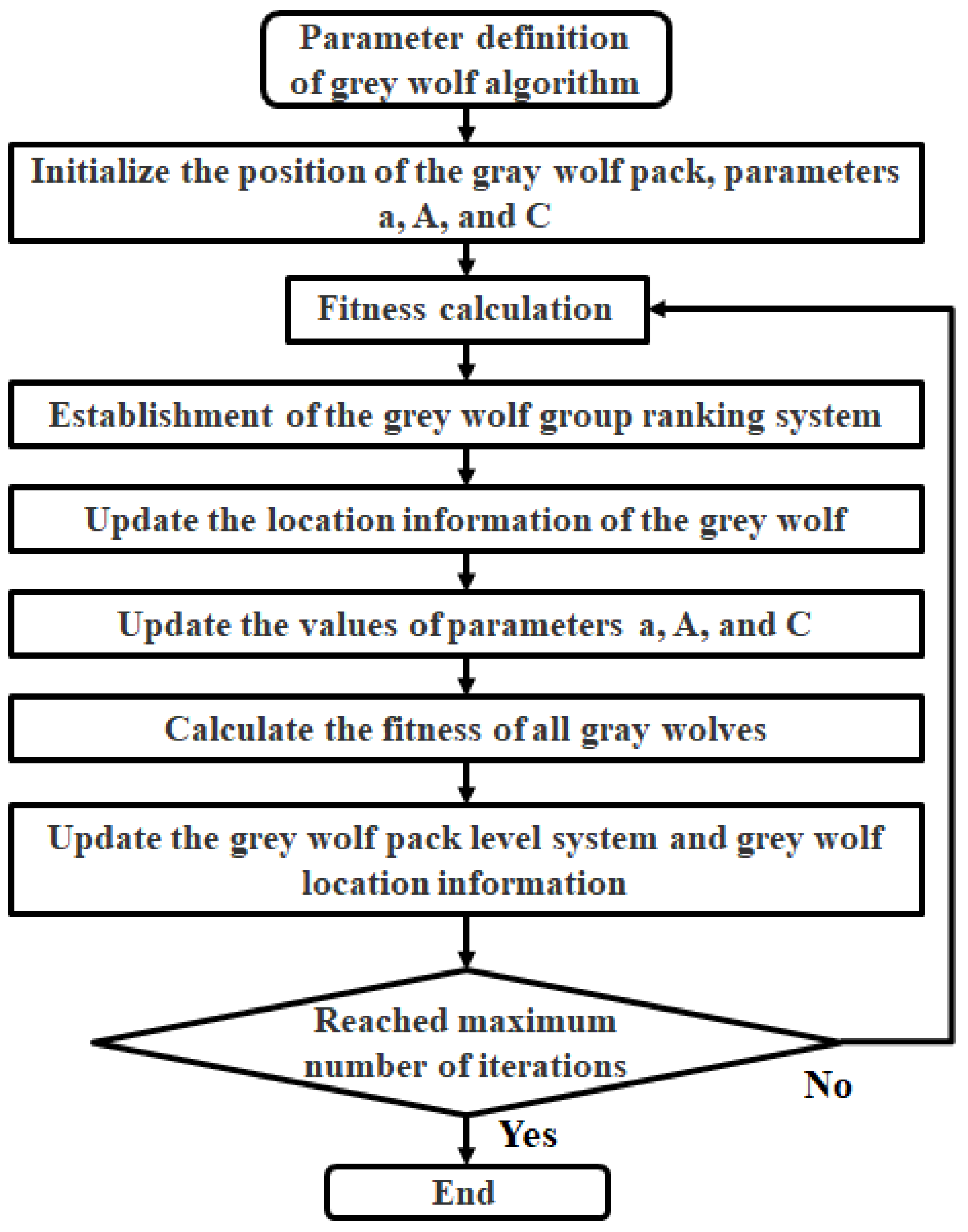
The grey wolf algorithm (GWO) is a method that seeks the optimal solution based on the hunting principle of a pack of grey wolves. It possesses advantages such as strong convergence, fewer parameters, simple structure, and ease of implementation. This paper takes power consumption as fitness, calculating the fitness of each grey wolf to establish a social hierarchy. Subsequently, the three wolves with the best fitness are selected as , , and , while the remaining wolves are labeled as . Its mathematical expression is shown in Equation (80), and the flowchart is illustrated in Figure 12.
In Equation (80): t represents the iteration count, and are cooperative coefficient matrices, denotes the prey’s location information, represents the wolves’ location information, is the convergence factor and gradually decreases from 2 to 0, and and are random variables within the range of [0, 1].
During the process of grey wolf hunting, the wolves can identify the prey’s location and encircle it. When the grey wolves identify the prey’s location, and , under the guidance of , lead the wolf pack to encircle the prey. To enhance the grey wolves’ ability to recognize potential prey, the fitness of the wolves is updated in each iteration calculation. The three wolves with the best fitness, designated as , , and , are chosen. Based on the position information of , , and , the position information of the remaining wolves is updated in the next iteration. The mathematical expressions are shown in Equations (81) and (82).
where X represents the current position of the grey wolf, is the distance between and the wolf, is the distance between and the wolf, is the distance between and the wolf, and , , and are random vectors.
where represents the position information of wolf , represents the position information of wolf , represents the position information of wolf , and denotes the updated positioning of the wolf.
The grey wolf algorithm (GWO) is used for offline optimization of the best braking distribution factor under various constraints. This process involves establishing a database correlating constraint sets with the optimal factors. During the vehicle’s actual operation, based on real-time vehicle speed and required braking force, the optimal factor is selected. This aims to enhance the vehicle’s fuel efficiency while meeting the overall braking demands of the vehicle.
4. Simulation and Evaluation
In this section, the effectiveness of the vehicle–road state observers, ENMPC braking force control strategy, and allocation of braking force sources is verified. To be specific, aiming to evaluate the performance of the vehicle state observer, the vehicle mass, road–tire adhesion coefficient, and vertical tire forces are assessed via comparing them with the data collected from the real-world driving test. Furthermore, to confirm the effectiveness of the ENMPC braking force control strategy, the proposed strategy is assessed via comparing it with a rule-based ABS strategy. Specially, a high-adhesion test and a low-adhesion test contrasted with a rule-based ABS strategy are provided to ensure that the ENMPC strategy can adapt to different road surfaces. Finally, to assess the adaptiveness of the proposed strategy utilizing the grey wolf algorithm, a test contrasting it with a rule-based distribution strategy is provided.
The mentioned rule-based strategies for ABS and distribution are as follows: The rule-based ABS strategy is a strategy that depends on the angular acceleration and the slip ratio threshold to increase or decrease the brake force. The rule-based brake force source distribution strategy is a strategy that uses a fixed distribution ratio to distribute the brake force from different sources.
For those verifications, a vehicle model is established consisting of a vehicle dynamics module, magic formula tire module, drive motor module, and battery pack module. The simulations are conducted on MATLAB R2021b and Python 3.8 and are performed on a personal computer equipped with an Intel i5-6300HQ processor and 8 GB of memory. Further, all simulations are conducted involving a fixed simulation step of 0.01 s.
4.1. Vehicle State Observer
The accuracy of the mass estimation, road adhesion estimation, and tire vertical force estimation results are verified in this section. The test conditions in this section are acceleration and deceleration from 0 to 60 to 0 km/h, with 0–30 s being the driving condition and 30–45 s being the braking condition.
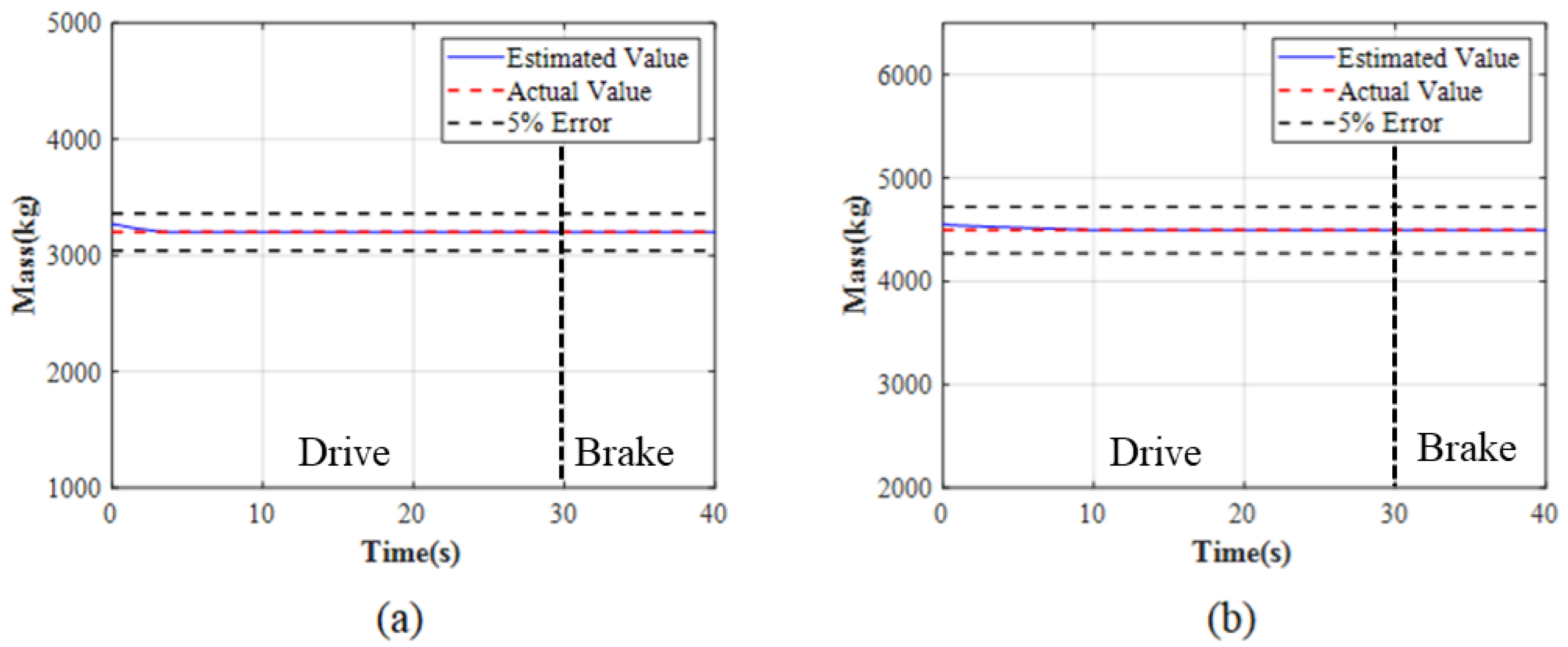
To ensure the effectiveness of the total braking force decision and tire vertical force estimation, the mass estimation results are verified. Figure 13 shows the mass estimation results, including the vehicle’s empty state (a) and full state (b).
To ensure the effectiveness of the total braking force decision-making and ENMPC control strategy, the road adhesion estimation is verified. Figure 14 shows the simulated road adhesion estimation results, including the high-adhesion road (a) and the low-adhesion road (b). The test conditions are high-intensity braking with ABS activation.
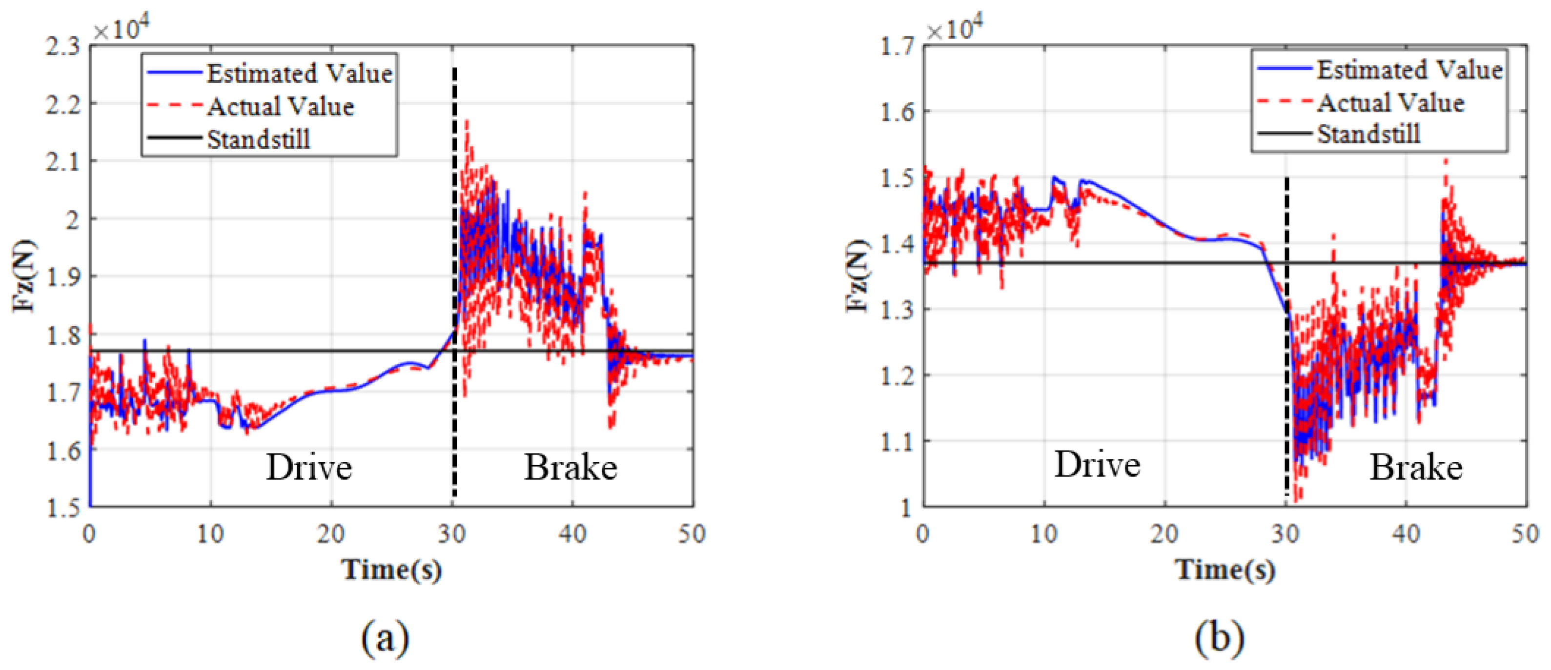
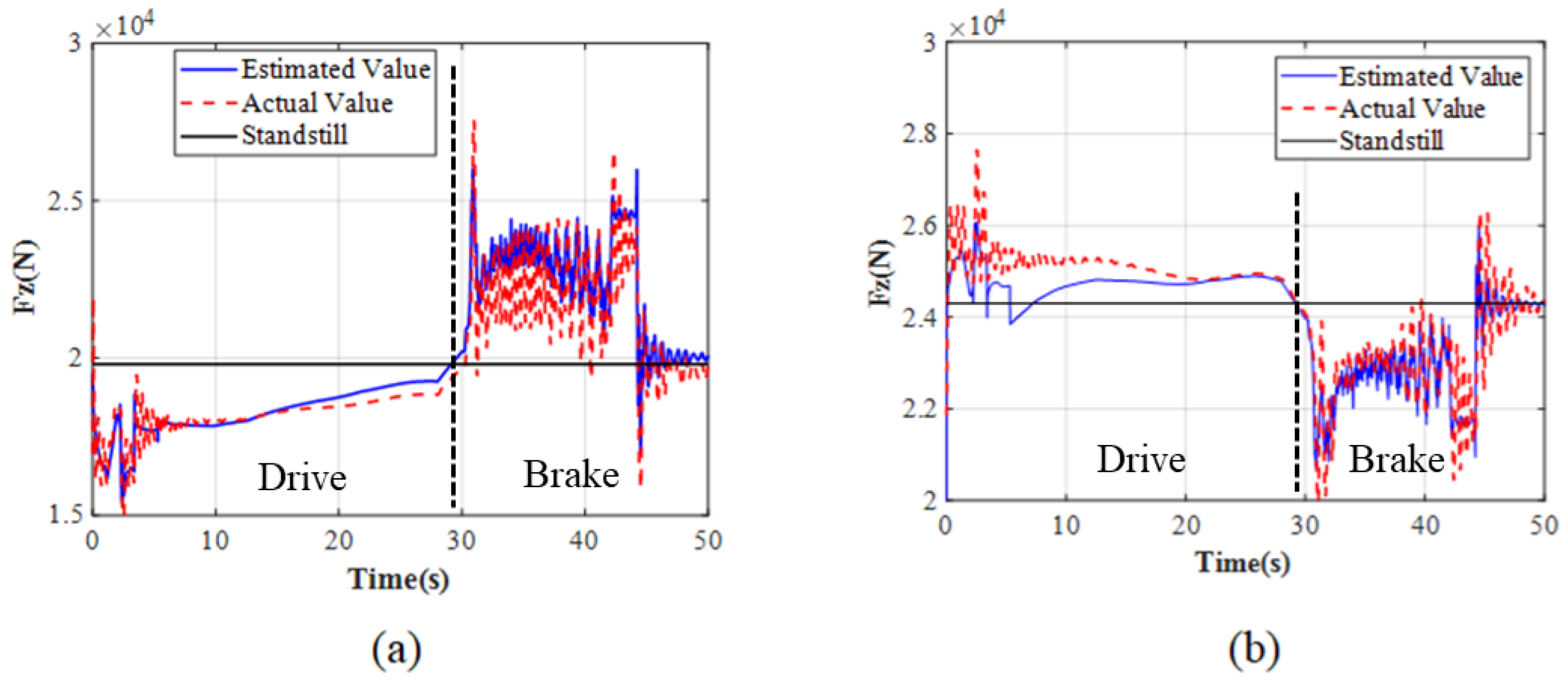
To ensure the effectiveness of inter-wheel braking, the tire vertical force estimation is verified through simulation. Figure 15 and Figure 16 show the simulated tire vertical force estimation results, including front axle with no load (Figure 15a), rear axle with no load (Figure 15b), front axle with full load (Figure 16a), and rear axle with full load (Figure 16b). “Standstill” indicates the tire vertical force when the vehicle is stationary.
As shown in Figure 13, regardless of full load or no load, the quality estimation can converge within 3 s and the error is less than 1%, which can meet the subsequent control requirements.
As shown in Figure 14, the error of road adhesion estimation reaches 5% on the high-adhesion road and 10% on the low-adhesion road. In the first 30 s, the road adhesion estimation cannot be estimated because the vehicle is in a non-braking state. The accuracy of road adhesion estimation affects the precision of total braking force decision-making and the EMPC control strategy.
As shown in Figure 15 and Figure 16, the error between the estimated value and the actual value is extremely small during the time period when ASR and ABS are not activated. During the time period when ASR (0–10 s) and ABS (30–40 s) are activated, there is significant fluctuation in the estimated and actual values due to the fluctuations of driving and braking torque and vehicle acceleration. However, the estimated and actual values have a consistent trend and fluctuate within their respective ranges. The result shows that the accuracy meets the requirements of subsequent control.
In conclusion, the errors in mass estimation, road adhesion estimation, and tire vertical force estimation are all within an acceptable range, laying the foundation for the development of subsequent ENMPC strategies.
4.2. ENMPC Braking Torque Control Strategy
In this section, the ENMPC-based braking torque control strategy is verified through simulation, and high- and low-adhesion road high-intensity braking tests are conducted.
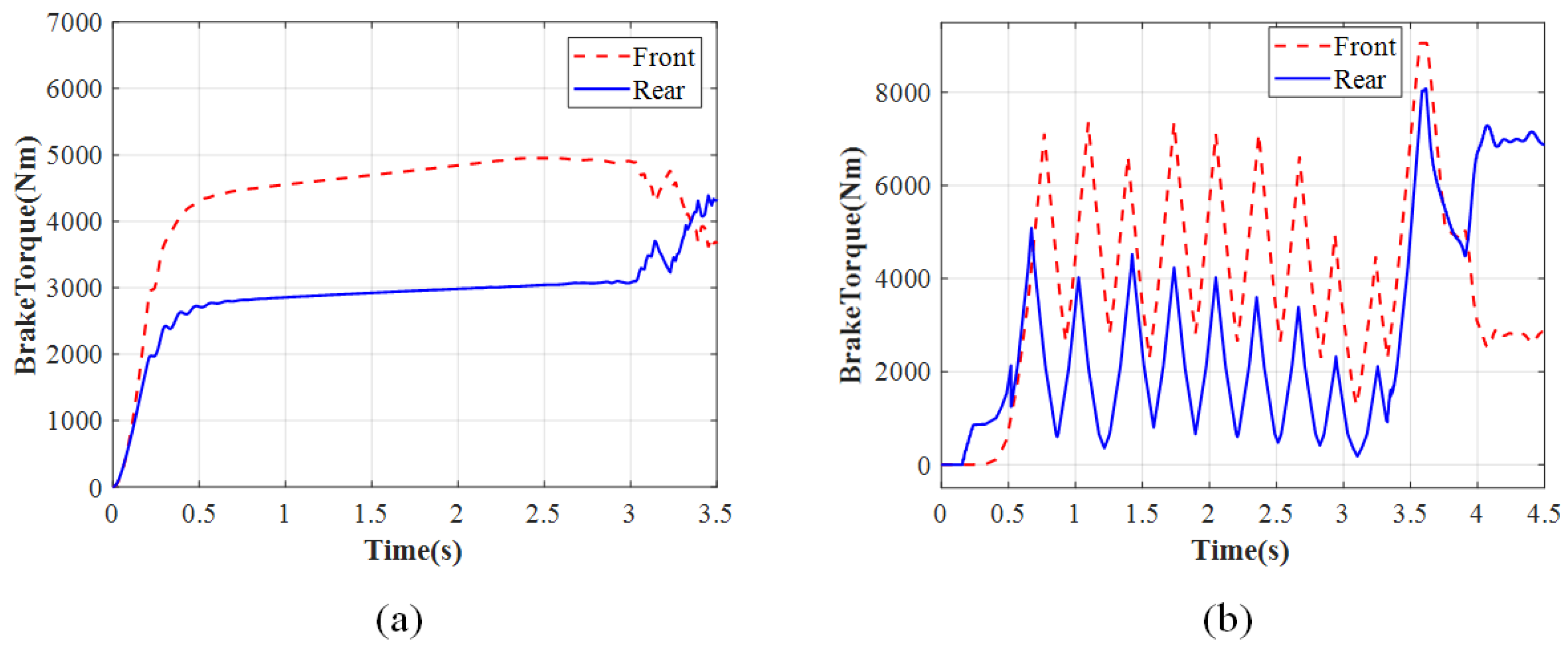
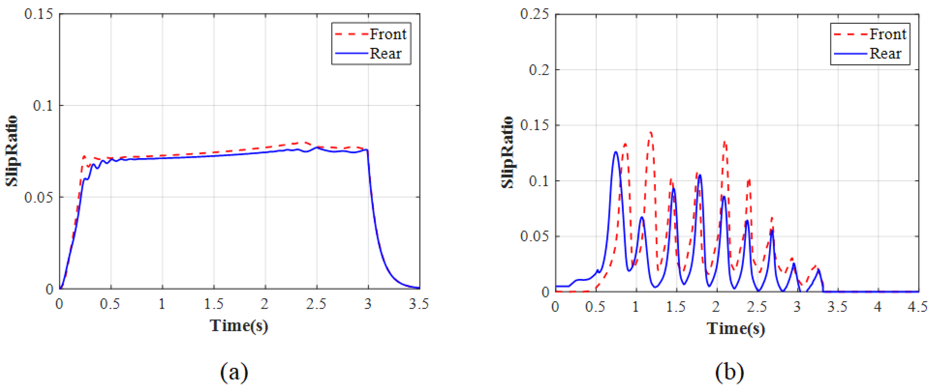
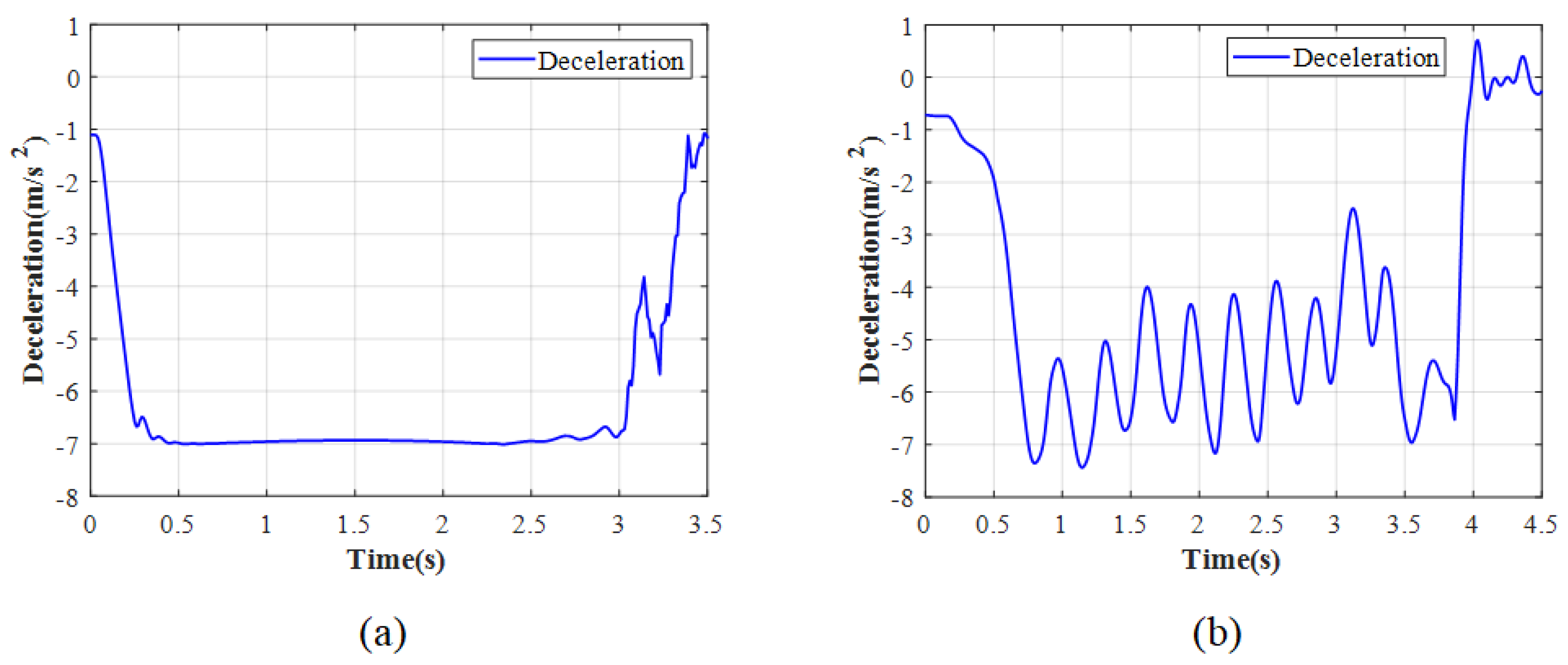
Table 2 shows the argument values of ENMPC in simulation. Figure 17, Figure 18, Figure 19 and Figure 20 show the simulation results of the ENMPC braking torque control strategy on a high-adhesion road. Under these conditions, the road adhesion is 0.8, the initial vehicle speed is 80 km/h, the desired slip ratio is 0.07, and the desired deceleration is approximately 7 m/s2. Figure 17a, Figure 18a, Figure 19a, and Figure 20a show the vehicle speed and wheel speed curves, braking torque curves, slip ratio curves, and deceleration curves, respectively, under the ENMPC strategy. Figure 17b, Figure 18b, Figure 19b, and Figure 20b show the vehicle speed and wheel speed curves, braking torque curves, slip ratio curves, and deceleration curves, respectively, under the rule-based ABS control strategy. Table 3 shows the braking time, average deceleration, and braking distance under both strategies.
As shown in Figure 17, Figure 18, Figure 19 and Figure 20, when comparing the braking torque curves of the ENMPC strategy and the rule-based ABS strategy, the rule-based ABS strategy relies on slip ratio and angular acceleration threshold values to control the boosting and releasing of the braking torque. Therefore, the rule-based strategy results in significant fluctuations in the braking torque, while the ENMPC strategy has a very fast convergence speed and does not experience large increases or decreases in the braking torque, which means this way is more suitable to control the braking torque by the drive motor. In the vehicle speed and wheel speed curves and slip ratio curves under the rule-based control, the large increase in braking torque corresponds to a decrease in wheel speed and an increase in slip ratio, while the large decrease in braking torque corresponds to an increase in wheel speed and a decrease in slip ratio. The slip ratio fluctuates repeatedly between 0 and 0.3. Under the ENMPC strategy, the braking torque is more stable due to the abandonment of traditional boosting and releasing strategies, and the corresponding slip ratio also stabilizes around the desired value of 0.07. Finally, when comparing the deceleration curves of the ENMPC strategy and the rule-based ABS strategy, due to the repeated fluctuations of the slip ratio between 0 and 0.3 under the rule-based ABS control, the utilization coefficient of each wheel also fluctuates repeatedly and only reaches its peak for a short period of time. Therefore, the deceleration fluctuates greatly and cannot reach a high level. However, under the ENMPC strategy, the slip ratio is maintained around 0.07, resulting in a consistent utilization coefficient for each wheel and a high deceleration of 7 m/s2.
In summary, the ENMPC control strategy not only allows for a high level of braking intensity but also ensures the safety of the vehicle during the braking process. Additionally, the stable demand for braking torque allows it to be provided by the drive motor rather than the EMB.
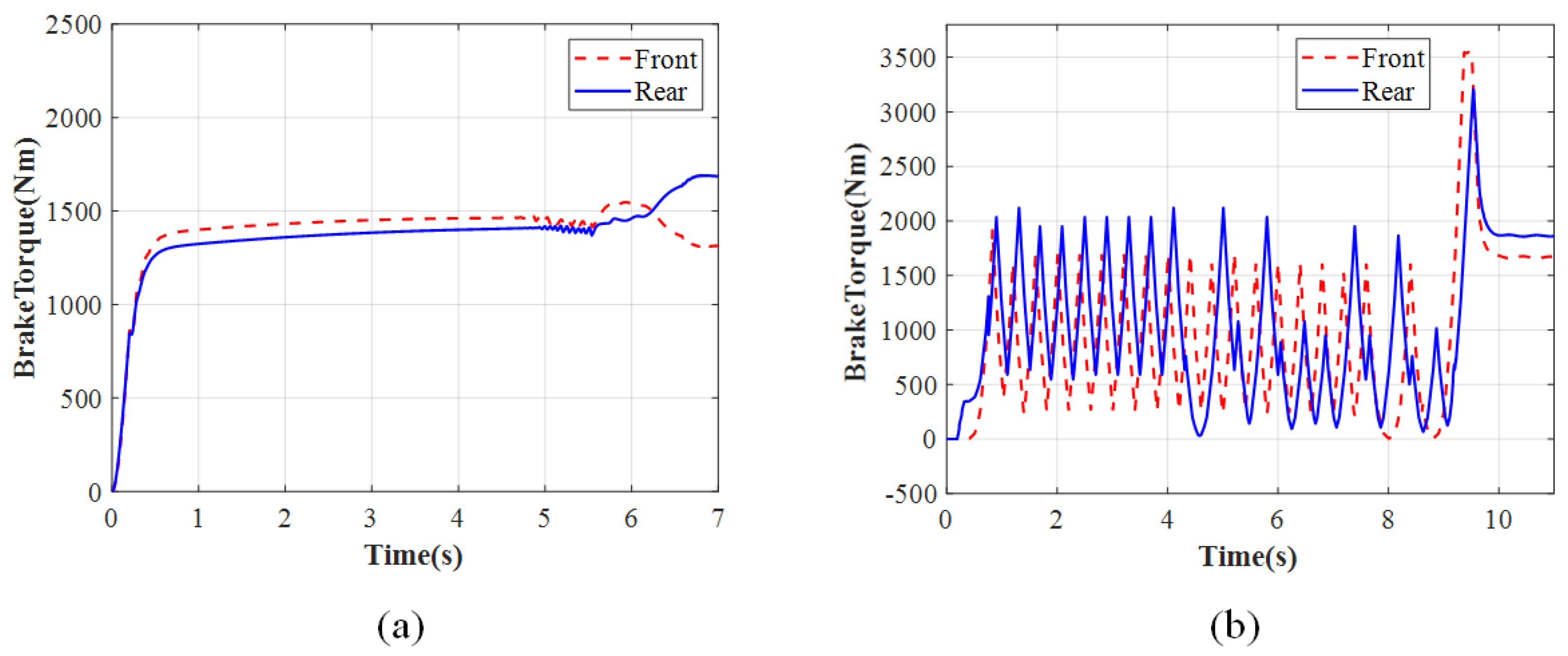
Figure 21, Figure 22, Figure 23 and Figure 24 show the simulation results of the ENMPC braking torque control strategy on a low-adhesion road. Under these conditions, the road adhesion is 0.3, the initial vehicle speed is 60 km/h, the desired slip ratio is 0.07, and the desired deceleration is approximately 3 m/s2. Figure 21a, Figure 22a, Figure 23a, and Figure 24a show the vehicle speed and wheel speed curves, braking torque curves, slip ratio curves, and deceleration curves, respectively, under the ENMPC strategy. Figure 21b, Figure 22b, Figure 23b, and Figure 24b show the vehicle speed and wheel speed curves, braking torque curves, slip ratio curves, and deceleration curves, respectively, under the rule-based ABS control strategy. Table 4 shows the braking time, average deceleration, and braking distance under both strategies.
As shown in Figure 21, Figure 22, Figure 23 and Figure 24, the simulation results on the low-adhesion road are similar to those on the high-adhesion road. Comparing the braking torque curves of the ENMPC strategy and the rule-based ABS strategy, the rule-based strategy results in significant fluctuations in the braking torque, while the ENMPC strategy has a very fast convergence speed and does not experience large increases or decreases in the braking torque even though the test is on the low-adhesion road, which means this way is more suitable to control the braking torque by the drive motor. In the vehicle speed, wheel speed curves, and slip ratio curves under the rule-based control, the slip ratio fluctuates repeatedly between 0 and 0.5. Under the ENMPC strategy, the braking torque is more stable due to the abandonment of traditional boosting and releasing strategies, and the corresponding slip ratio also stabilizes around the desired value of 0.07. Finally, when comparing the deceleration curves of the ENMPC strategy and the rule-based ABS strategy, due to the repeated fluctuations of the slip ratio between 0 and 0.5 under the rule-based ABS control, the deceleration fluctuates greatly and cannot reach a high level. However, under the ENMPC strategy, the slip ratio is maintained around 0.07, resulting in a consistent utilization coefficient for each wheel and a high deceleration of 3 m/s2.
Similar to the results on the high-adhesion road, the EMPC strategy on the low-adhesion road also allows the braking torque to be provided by the drive motor rather than the EMB and provides stable demand for braking torque.
In summary, whether on a high-adhesion road or a low-adhesion road, the ENMPC strategy outperforms the traditional rule-based ABS control strategy in terms of braking intensity, safety, and energy efficiency.
4.3. Allocation of Braking Force Sources
To ensure the energy recovery of the drive motor and the rational allocation between the energy-consuming braking of the drive motor and the mechanical braking of the EMB, this section simulates and verifies the braking source allocation strategy.
In this paper, the number of wolves is 20, and 100 iterations are selected. Figure 25 and Figure 26 show the braking torque of each braking source and the energy obtained by the battery during braking. Figure 25a and Figure 26a show the braking torque curves of each braking source and the battery energy curves under the grey wolf allocation strategy, while Figure 25b and Figure 26b show the braking torque curves of each braking source and the battery energy curves under the rule-based allocation strategy. Under this condition, the vehicle is braking at any intensity and with a simulated deceleration of 2 m/s2. The front axle braking force is provided solely by the EMB, while the rear axle braking force is provided by the energy recovery of the drive motor, energy-consuming braking of the drive motor, and the EMB. Therefore, the analysis of the braking source allocation focuses on the rear axle.
As shown in Figure 25a, under the rule-based allocation strategy, the braking force is provided by a fixed ratio between energy recovery of the drive motor and the EMB. Therefore, during high-speed braking, the braking force is provided by the energy recovery of the drive motor and the EMB, while at low speeds, the drive motor cannot recover energy and instead uses energy-consuming braking to provide the braking force.
As shown in Figure 25b, comparing the energy obtained during braking, the grey wolf allocation strategy results in significantly more energy recovered due to the increased involvement of energy recovery of the drive motor, far surpassing the rule-based strategy. The grey wolf algorithm possesses advantages such as strong convergence, fewer parameters, simple structure, and ease of implementation. The fitness is taken by power consumption, which means the less power consumed, the more energy obtained for the battery. The grey wolf algorithm find a way to consume less energy, which means letting the motor regeneration torque maximize its value.
As shown in Figure 26, due to the grey wolf allocation applying more motor regeneration torque than the rule-based distribution strategy, the grey wolf allocation can obtain more energy for the battery. When the vehicle brakes at a low velocity, the motor cannot provide enough motor regeneration torque for the tires, so neither the grey wolf allocation nor the rule-based distribution strategy can obtain more energy for the battery, instead, the motor consume the energy to obtain a braking torque for the tires in order to stop the vehicle.
In summary, the grey wolf allocation strategy can obtain more energy for the battery, so it surpasses the rule-based distribution strategy in terms of energy efficiency. It should be noted that the ENMPC brake force control strategy provides stable braking force and allows the brake force source distribution to have an opportunity to explore more feasible methods to enhance the energy efficiency.
5. Conclusions
In this paper, a multi-source braking force system and its control strategy is proposed, with the aim of improving the braking intensity, safety, and energy efficiency of the braking process. The vehicle–road state observer makes the parameter accurate enough, resulting in less than a 10 percent error, in order to meet the requirements of subsequent control. An ENMPC-based brake force control strategy is developed and integrated into the proposed strategy, accomplishing the stable braking force required instead of the traditional ABS strategy, which requires a repeated fluctuation force. Additionally, a grey wolf allocation is designed to achieve the distribution of the brake force from different sources, with the aim of enhancing energy efficiency. Furthermore, the simulation results highlight the improvement to the braking intensity, safety, and energy efficiency of the proposed strategy. Compared to the traditional ABS strategy, the strategy in this paper increases the braking intensity 25 percent on high-adhesion surfaces and 54 percent on low-adhesion surfaces and reduces the fluctuation of the slip ratio by about 50 percent during the braking process. Meanwhile, the strategy in this paper increases the amount of energy recovered by the battery by about 60 percent during the braking process compared with the traditional brake source distribution.
In summary, this paper analyzes the feasibility of power-consuming braking of the drive motor, studies braking force control under emergency braking, improves braking efficiency and braking stability, studies the distribution of braking force sources, and improves the energy recovery rate.
However, the control strategy in this paper does not consider uneven-adhesion road, such as docking and splitting road surfaces. Furthermore, this paper only focuses on distributed-brake centralized-drive vehicles and does not analyze vehicles with a distributed-drive configuration. Moreover, this paper has not verified the safety of the motor brake compensation. In future work, these issues will be considered to improve the strategy.
Author Contributions
Conceptualization, Y.W., L.Z., L.C., D.Z., Z.G. and Z.J.; Methodology, Y.W., L.Z., D.Z., Z.G. and Z.J.; Software, Y.W., L.Z., D.Z. and Z.G.; Validation, Y.W., L.Z. and Z.J.; Formal analysis, Y.W. and L.Z.; Investigation, Y.W. and L.Z.; Resources, Y.W., L.Z. and D.Z.; Data curation, Y.W. and L.Z.; Writing—original draft, Y.W. and L.Z.; Writing—review & editing, Y.W. and L.Z.; Visualization, Y.W. and L.Z.; Supervision, Y.W. and L.Z.; Project administration, Y.W. and L.Z.; Funding acquisition, Y.W. and L.Z. All authors have read and agreed to the published version of the manuscript.
Funding
This research received no external funding.
Data Availability Statement
The original contributions presented in the study are included in the article, further inquiries can be directed to the corresponding authors.
Conflicts of Interest
The authors declare no conflict of interest.
References
- Gao, Y.; Ehsani, M. Electronic Braking System of EV and HEV—Integration of Regenerative Braking, Automatic Braking Force Control and ABS; SAE Technical Papers; SAE International: Warrendale, PA, USA, 2001. [Google Scholar]
- Nakamura, E.; Soga, M.; Sakai, A.; Otomo, A.; Kobayashi, T. Development of Electronically Controlled Brake System for Hybrid Vehicle; SAE Technical Papers; SAE International: Warrendale, PA, USA, 2002. [Google Scholar]
- Joon, K.S.; Woochul, L.; Jung, D. Electro-Mechanical Brake. KR Patent 102401769B1, 25 May 2022. [Google Scholar]
- Li, C.; Zhuo, G.; Tang, C.; Xiong, L.; Tian, W.; Qiao, L.; Cheng, Y.; Duan, Y. A review of electro-mechanical brake(EMB) system: Structure, control and application. Sustainability 2023, 15, 4514. [Google Scholar] [CrossRef]
- Maron, C.; Georg, R. Method for Actuating an Electromechanical Parking Brake Device. US Patent 2006131113A1, 22 June 2006. [Google Scholar]
- Michael, H. Bremseinrichtung mit einem Keilmechanismus. DE Patent 102007013421A1, 25 September 2008. [Google Scholar]
- Yang, L.; Sun, S.; Qin, Z.; Shan, G.; Han, Z. Automatic Generation Analysis Method of Automobile Chassis Electronic Control System Based on NLP-intelligent Control Condition. In Proceedings of the 2023 38th Youth Academic Annual Conference of Chinese Association of Automation (YAC), Hefei, China, 27–29 August 2023; pp. 514–519. [Google Scholar]
- Saiteja, P.; Ashok, B.; Wagh, A.S.; Farrag, M.E. Critical review on optimal regenerative braking control system architecture, calibration parameters and development challenges for EVs. Int. J. Energy Res. 2022, 46, 20146–20179. [Google Scholar] [CrossRef]
- Satzger, C.; de Castro, R. Predictive brake control for electric vehicles. IEEE Trans. Veh. Technol. 2017, 67, 977–990. [Google Scholar] [CrossRef]
- Lee, C.F. Brake Force Control and Judder Compensation of an Automotive Electromechanical Brake. Doctoral Dissertation, University of Melbourne, Department of Mechanical Engineering, Melbourne, Australia, 2013. [Google Scholar]
- Li, J.; Wu, T.; Fan, T.; He, Y.; Meng, L.; Han, Z. Clamping force control of electro–mechanical brakes based on driver intentions. PLoS ONE 2020, 15, e0239608. [Google Scholar] [CrossRef] [PubMed]
- Tao, Y.; Xie, X.; Zhao, H.; Xu, W.; Chen, H. A Regenerative Braking System for Electric Vehicle with Four in-Wheel Motors Based on Fuzzy Control. In Proceedings of the Chinese Control Conference, Dalian, China, 26–28 July 2017. [Google Scholar]
- Sun, Y.; Wang, Y.; Zhu, R.; Geng, R.; Zhang, J.; Fan, D.; Wang, H. Study on the Control Strategy of Regenerative Braking for the Hybrid Electric Vehicle under Typical Braking Condition. Iop Conf. Ser. Mater. Sci. Eng. 2018, 452, 032092. [Google Scholar] [CrossRef]
- Xu, Q.; Wang, F.; Zhang, X. Research on the Efficiency Optimization Control of the Regenerative Braking System of Hybrid Electrical Vehicle Based on Electrical Variable Transmission. IEEE Access 2019, 7, 116823–116834. [Google Scholar] [CrossRef]
- Gao, H.; Gao, Y.; Ehsani, M. A Neural Network Based SRM Drive Control Strategy for Regenerative Braking in EV and HEV. In Proceedings of the IEMDC 2001, IEEE International Electric Machines and Drives Conference (Cat. No.01EX485), Cambridge, MA, USA, 17–20 June 2001. [Google Scholar]
- Wang, C.; Zhao, W.; Li, W. Braking Sense Consistency Strategy of Electro-Hydraulic Composite Braking System. Mech. Syst. Signal Process. 2018, 109, 196–219. [Google Scholar] [CrossRef]
- Savaresi, M.S.; Tanelli, M. Active Braking Control System Design for Vehicles; Springer: New York, NY, USA, 2010. [Google Scholar]
- Aly, A.A.; Zeidan, E.-S.; Hamed, A.; Salem, F. An antilock-braking systems (ABS) control: A technical review. Intell. Control Autom. 2011, 2, 186–195. [Google Scholar] [CrossRef]
- Choi, S.B. Antilock brake system with a continuous wheel slip control to maximize the braking performance and the ride quality. IEEE Trans. Control Syst. Technol. 2008, 16, 996–1003. [Google Scholar] [CrossRef]
- Yin, D.; Oh, S.; Hori, Y. A novel traction control for EV based on maximum transmissible torque estimation. IEEE Trans. Ind. Electron. 2009, 56, 2086–2094. [Google Scholar]
- Wang, Y.; Fujimoto, H.; Hara, S. Driving force distribution and control for EV with four in-wheel motors: A case study of acceleration on splitfriction surfaces. IEEE Trans. Ind. Electron. 2017, 64, 3380–3388. [Google Scholar] [CrossRef]
- Yoo, D.; Wang, L. Model based wheel slip control via constrained optimal algorithm. In Proceedings of the 2007 IEEE International Conference on Control Applications, Singapore, 1–3 October 2007; pp. 1239–1246. [Google Scholar]
- Borrelli, F.; Bemporad, A.; Fodor, M.; Hrovat, D. An MPC/hybrid system approach to traction control. IEEE Trans. Control Syst. Technol. 2006, 14, 541–552. [Google Scholar] [CrossRef]
- Tavernini, D.; Metzler, M.; Gruber, P.; Sorniotti, A. Explicit nonlinear model predictive control for electric vehicle traction control. IEEE Trans. Contr. Syst. Technol. 2018; to be published. [Google Scholar] [CrossRef]
- von Albrichsfeld, C.; Karner, J. Brake System for Hybrid and Electric Vehicles; SAE Technical Paper; SAE International: Warrendale, PA, USA, 2009. [Google Scholar]
- Conlon, B.M.; Kidston, K.S. Electric Vehicle with Regenerative and Anti-lock Braking. U.S. Patent 5,615,933, 1 April 1997. [Google Scholar]
- Schneider, M.; Shaffer, A. Regenerative Braking Control System and Method. U.S. Patent Application 11/164,195, 14 November 2005. [Google Scholar]
- Hori, Y. Future Vehicle Driven by Electricity and Control research on Four-wheel-motored “UOT Electric March II”. IEEE Trans. Ind. Electron. 2004, 51, 954–962. [Google Scholar] [CrossRef]
- Hsiao, M.; Lin, C. Antilock Braking Control of Electric Vehicles with Electric Brake; SAE Technical Paper; SAE International: Warrendale, PA, USA, 2005. [Google Scholar]
- Tur, O.; Ustun, O.; Tuncay, R.N. An Introduction to Regenerative Braking of Electric Vehicles as Anti-lock Braking System. In Proceedings of the 2007 Intelligent Vehicles Symposium, Istanbul, Turkey, 13–15 June 2007; pp. 944–948. [Google Scholar]
- Okano, T.; Sakai, S.; Uchida, T.; Hori, Y. Braking Performance Improvement for Hybrid Electric Vehicle Based on Electric Motor’s Quick Torque Response. In Proceedings of the 19th International Electric Vehicle Symposium (EVS19), Busan, Republic of Korea, 19–23 October 1999. [Google Scholar]
- Zhang, J.Z.; Chen, X.; Zhang, P.J. Integrated Control of Braking Energy Regeneration and Pneumatic Anti-lock Braking. J. Automob. Eng. 2010, 224, 587–610. [Google Scholar] [CrossRef]
- Zhang, J.; Kong, D.; Chen, L.; Chen, X. Optimization of Control Strategy for Regenerative Braking of an Electrified Bus Equipped with an Anti-lock Braking System. J. Automob. Eng. 2012, 226, 494–506. [Google Scholar] [CrossRef]
- Bayar, K.; Wang, J.; Rizzoni, G. Development of a Vehicle Stability Control Strategy for a Hybrid Electric Vehicle Equipped with Axle Motors. J. Automob. Eng. 2012, 226, 795–814. [Google Scholar] [CrossRef]
- Liu, Y.; Dou, C. Vehicle State Estimation Based on Unscented Kalman Filtering and a Genetic Algorithm. SAE Int. J. Commer. Veh. 2020, 14, 23–37. [Google Scholar] [CrossRef]
- Wu, D.; Zeng, C.; Luo, J. Research on Joint Estimation Algorithm of Intelligent Vehicle Mass and Road Grade. In Proceedings of the 2023 4th International Conference on Computer Engineering and Application (ICCEA), Hangzhou, China, 7–9 April 2023. [Google Scholar]
- Rodríguez, A.J.; Sanjurjo, E.; Pastorino, R.; Naya, M.Á. State, parameter and input observers based on multibody models and Kalman filters for vehicle dynamics. Mech. Syst. Signal Process. 2021, 155, 107544. [Google Scholar]
- Basrah, M.S.; Siampis, E.; Velenis, E.; Cao, D.; Longo, S. Wheel slip control with torque blending using linear and nonlinear model predictive control. Veh. Syst. Dyn. 2017, 55, 1665–1685. [Google Scholar]
- Yuan, L.; Zhao, H.; Chen, H.; Ren, B. Nonlinear MPC-based slip control for electric vehicles with vehicle safety constraints. Mechatronics 2016, 38, 1–15. [Google Scholar] [CrossRef]
- Satzger, C.; de Castro, R.; Knoblach, A.; Brembeck, J. Design and validation of anMPC-based torque blending and wheel slip control strategy. In Proceedings of the 2016 IEEE Intelligent Vehicles Symposium (IV), Gothenburg, Sweden, 19–22 June 2016; Volume 2016, pp. 514–520. [Google Scholar]
- Pei, X.; Pan, H.; Chen, Z.; Guo, X.; Yang, B. Coordinated control strategy of electro-hydraulic braking for energy regeneration. Control Eng. Pract. 2020, 96, 104324. [Google Scholar] [CrossRef]
- Li, N.; Ning, X.; Wang, Q. Genetic Algorithm Optimization of Hydraulic Regenerative Braking System for Electric Vehicles. Bol. Tec. 2017, 55, 513–523. [Google Scholar]
- Zheng, X.; Gao, X.; Zhao, Z. Simulation Analysis of Tire Dynamic Based on “Magic Formula”. Mach. Electron. 2012, 9, 16–20. [Google Scholar]
Figure 1.
Braking torque from different sources.

Figure 2.
Vehicle electronic control system architecture.

Figure 3.
EMB response characteristics.

Figure 4.
The motor’s external characteristics.

Figure 5.
Braking force control strategy process.

Figure 6.
The relationship between motor torque and speed.

Figure 7.
The relationship between deceleration and brake torque.

Figure 8.
The relationship between deceleration and brake torque for different adhesion coefficients.
Figure 8.
The relationship between deceleration and brake torque for different adhesion coefficients.

Figure 9.
Nonlinear model predictive control process.

Figure 10.
Explicit process.

Figure 11.
Different parts divided by velocity and brake torque.

Figure 12.
The grey wolf algorithm process.

Figure 13.
Mass estimate results: (a) No load. (b) Full load.

Figure 14.
Adhesion coefficient estimates: (a) High adhesion. (b) Low adhesion.

Figure 15.
Vertical tire forces for no load: (a) Front axle. (b) Rear axle.

Figure 16.
Vertical tire forces for full load: (a) Front axle. (b) Rear axle.

Figure 17.
Vehicle and wheel speed for high adhesion: (a) ENMPC strategy. (b) Rule-based ABS strategy.
Figure 17.
Vehicle and wheel speed for high adhesion: (a) ENMPC strategy. (b) Rule-based ABS strategy.

Figure 18.
Brake torque for high adhesion: (a) ENMPC strategy. (b) Rule-based ABS strategy.

Figure 19.
Slip ratio for high adhesion: (a) ENMPC strategy. (b) Rule-based ABS strategy.

Figure 20.
Deceleration for high adhesion: (a) ENMPC strategy. (b) Rule-based ABS strategy.

Figure 21.
Vehicle and wheel speed for low adhesion: (a) ENMPC strategy. (b) Rule-based ABS strategy.
Figure 21.
Vehicle and wheel speed for low adhesion: (a) ENMPC strategy. (b) Rule-based ABS strategy.

Figure 22.
Brake torque for low adhesion: (a) ENMPC strategy. (b) Rule-based ABS strategy.

Figure 23.
Slip ratio for low adhesion: (a) ENMPC strategy. (b) Rule-based ABS strategy.

Figure 24.
Deceleration for low adhesion: (a) ENMPC strategy. (b) Rule-based ABS strategy.

Figure 25.
Brake torque from each sources: (a) Grey wolf strategy. (b) Rule-based distribution strategy.
Figure 25.
Brake torque from each sources: (a) Grey wolf strategy. (b) Rule-based distribution strategy.

Figure 26.
Energy obtained: (a) Grey wolf strategy. (b) Rule-based distribution strategy.


Table 1.
Vehicle Parameter.
| Definition | Unit | Value |
|---|---|---|
| Vehicle mass (full) | kg | 4495 |
| Vehicle mass (no load) | kg | 3200 |
| Front axle load (full) | kg | 2000 |
| Front axle load (no load) | kg | 1800 |
| Rear axle load (full) | kg | 2495 |
| Rear axle load (no load) | kg | 1400 |
| Height of vehicle c.g. (full) | mm | 844 |
| Height of vehicle c.g. (no load) | mm | 630 |
| Distance between two axles | mm | 3300 |
| Wheel type | - | 750R16 |
Table 2.
The argument values of ENMPC.
| Argument | Value |
|---|---|
| t | 3 |
| q1 | |
| q2 | |
| q3 | |
| r1 | 1 |
| r2 | 1 |
| r3 | 1 |
| 200 | |
| 50 | |
| 150 | |
| 200 |
Table 3.
Details of high-adhesion braking.
| Definition | Unit | Value (ENMPC) | Value (Rule-Based) |
|---|---|---|---|
| Braking time | s | 3.4 | 4 |
| Average deceleration | m/s2 | 6.96 | 5.56 |
| Braking distance | m | 37.2 | 44.6 |
Table 4.
Details of low-adhesion braking.
| Definition | Unit | Value (ENMPC) | Value (Rule-Based) |
|---|---|---|---|
| Braking time | s | 6.4 | 10.6 |
| Average deceleration | m/s2 | 2.67 | 1.73 |
| Braking distance | m | 56.4 | 91.2 |
Disclaimer/Publisher’s Note: The statements, opinions and data contained in all publications are solely those of the individual author(s) and contributor(s) and not of MDPI and/or the editor(s). MDPI and/or the editor(s) disclaim responsibility for any injury to people or property resulting from any ideas, methods, instructions or products referred to in the content. |
© 2024 by the authors. Licensee MDPI, Basel, Switzerland. This article is an open access article distributed under the terms and conditions of the Creative Commons Attribution (CC BY) license (https://creativecommons.org/licenses/by/4.0/).
Share and Cite
MDPI and ACS Style
Wang, Y.; Zhou, L.; Chu, L.; Zhao, D.; Guo, Z.; Jiang, Z. A Multi-Source Braking Force Control Method for Electric Vehicles Considering Energy Economy. Energies 2024, 17, 2032. https://0-doi-org.brum.beds.ac.uk/10.3390/en17092032
AMA Style
Wang Y, Zhou L, Chu L, Zhao D, Guo Z, Jiang Z. A Multi-Source Braking Force Control Method for Electric Vehicles Considering Energy Economy. Energies. 2024; 17(9):2032. https://0-doi-org.brum.beds.ac.uk/10.3390/en17092032
Chicago/Turabian StyleWang, Yinhang, Liqing Zhou, Liang Chu, Di Zhao, Zhiqi Guo, and Zewei Jiang. 2024. "A Multi-Source Braking Force Control Method for Electric Vehicles Considering Energy Economy" Energies 17, no. 9: 2032. https://0-doi-org.brum.beds.ac.uk/10.3390/en17092032
Note that from the first issue of 2016, this journal uses article numbers instead of page numbers. See further details here.