
An Efficient Methodology to Identify Relevant Multiple Contingencies and Their Probability for Long-Term Resilience Studies


Ricerca sul Sistema Energetico—RSE S.p.A., 20134 Milano, Italy
*
Author to whom correspondence should be addressed.
Energies 2024, 17(9), 2028; https://0-doi-org.brum.beds.ac.uk/10.3390/en17092028
Submission received: 31 March 2024
/
Revised: 10 April 2024
/
Accepted: 17 April 2024
/
Published: 25 April 2024
(This article belongs to the Section F1: Electrical Power System)
Abstract
:The selection of multiple contingency scenarios is a key task to perform resilience-oriented long-term planning analyses. However, the identification of relevant multiple contingencies may easily lead to combinatorial explosion issues, even for relatively small systems. This paper proposes an effective methodology for the identification of relevant multiple contingencies and their probabilities, suitable for the long-term resilience analysis of large power systems. The methodology is composed of two main pillars: (1) the clustering of lines that are more likely to fail together, to reduce the computational complexity of the analysis exploiting historical weather data and (2) the probability-based identification of multiple contingencies within each cluster, where the contingency probability is computed applying the copula theory. Tests performed on a portion of the Italian EHV transmission system confirm the validity of the clustering results compared against historical failure events. Moreover, the copula-based algorithm for contingency probability estimation passes the tests carried out on relatively large clusters with very low error tolerance. The method successfully pinpoints critical multiple contingency scenarios and their likelihoods, making it valuable for assessing power system resilience over long-term horizons in support of resilience-oriented planning activities.
1. Introduction
Traditionally, power system reliability assessment has focused on identifying potential failure scenarios to quantify the ability of the system to deliver energy to customers within specified standards [1]. However, resilience assessment goes beyond this, as it requires pinpointing in a rapid and robust way the most representative contingency scenarios, i.e., those disruptions that are most likely to occur and have a significant impact [2]. In recent years, resilience has been investigated in many research activities, as shown in [3,4]. This is critical, because resilience assessment requires analyzing a multitude of potential disruptions, from natural disasters to equipment failures. In the literature, most references [2,3,5] adopt a Monte Carlo sampling (MCS) method to generate failure scenarios, i.e., the failures (OFF state) of components are extracted considering specific failure probabilities in the sampling process, also including correlations among component failures such as during severe weather events. Such a method is very time consuming, especially for large power systems, even though variance reduction techniques can be used to reduce the time to convergence, such as the importance sampling [6] or stratified sampling techniques [7]. In [8], a cross-entropy (CE)-based optimization process is combined with nonsequential Monte Carlo simulation (MCS) in order to obtain an auxiliary sampling distribution, which can minimize the variance of the reliability index estimators. Other references suggest the adoption of the subset simulation method, either alone [9] or in combination with CE optimization [10], to speed up the conventional MCS. Alternatively, “analytical” methods exist, such as Markov cutset methods [11], state space methods [12] and enumeration methods [13]. The first methods, based on the application of Markov processes to cutsets, require the elaboration of the Markov transition matrix from normal to adverse weather, and their search space is intrinsically limited by the maximum cardinality (hardly higher than 3) of the considered cutsets. The second category of methods is based on a state-space-pruning-based intelligent search and requires the tuning of the parameters for heuristic algorithms to select the most critical contingencies. Enumeration methods limit the number of contingencies to be analyzed according to specific criteria (e.g., probability of occurrence, severity); they are simpler than state space methods and their search space may be larger than the one of the Markov cutset methods. MCS methods are usually more time consuming than enumeration methods, but they are also more accurate in case of a sufficiently high number of samples to assure its convergence. Moreover, traditional enumeration methods are limited to a set of low-order contingencies due to combinatorial explosion issues; thus, they cannot capture the higher-order contingencies that are usually the focus of resilience analyses. Some techniques have been proposed to identify multiple contingencies, such as minimum cutsets [14], random chemistry [15] and graph theory [16], but they usually rank the contingencies only based on their impacts, thus overlooking their likelihood, which could be derived from a historical series of past extreme events. Recently, semi-analytical Monte Carlo methods for rare event sampling have also been proposed in the literature [17] to join the benefits of these two categories of methods (the speed of analytical methods with the accuracy of Monte Carlo sampling), even if no application to resilience analyses has been reported and only low-order contingencies have been simulated in the case studies.
The added value of the present paper is to propose an innovative method to identify, and estimate the long-term probability of, the most representative multiple contingencies potentially affecting grid components in large power systems during extreme weather events while also exploiting data from past weather events. This represents an important step forward in the application of enumeration methods in resilience assessment.
The paper is organized as follows: Section 2 briefly presents the requirements and the architecture of the proposed methodology. Section 3 and Section 4 describe the two main pillars composing the methodology, namely the clustering of grid components and the probability-based selection of the contingencies, respectively. Section 5 discusses some tests on the methodology on a realistic set of lines from a real-world power system. Section 6 concludes.
2. The Proposed Methodology
This section presents the context and the general approach of the proposed contingency identification method.
2.1. The Context: The RELIEF Risk-Based Resilience Assessment Framework
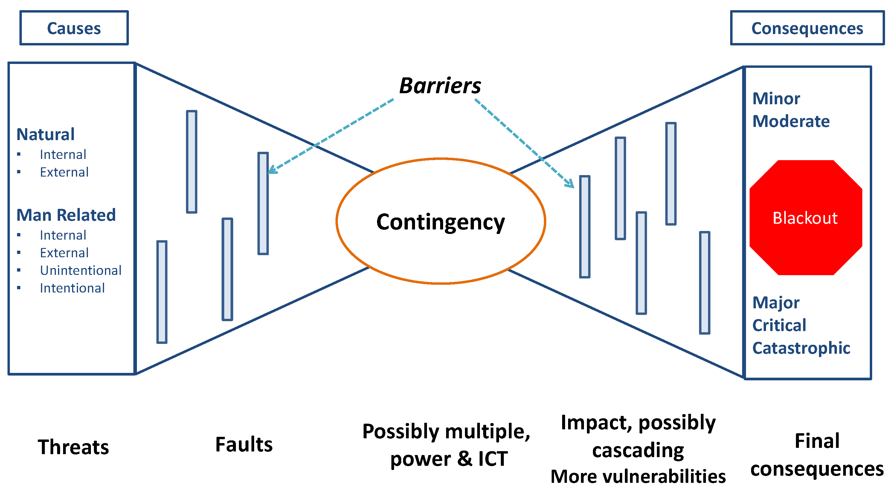
Resilience was defined by CIGRE WG C4.47 [18] as “the ability to limit the extent, severity and duration of system degradation following an extreme event”. Accordingly, analyzing resilience implies the modeling of the complex relationships between the power system and the (natural and human) environment. In fact, a resilience assessment process begins by modeling the root causes (e.g., wet snowstorm) of the failures, i.e., natural or man-made threats. To this goal, Figure 1 shows the conceptual bowtie model used to show the connections between threats, component vulnerabilities and power system contingencies and their impact within the risk-based resilience assessment framework RELIEF (REsiLIEnce measures For the grid) developed by RSE [1,19].
A thorough discussion of this conceptual scheme is presented in [19]. It is worth recalling that the threats (indicated on the left) strike power system components via stress variables (e.g., wind speed for wind threat) and they provoke the faults of components by exploiting their vulnerabilities. These faults can lead to a contingency whose impact also depends on the response of protection, control, defense and automation systems. The impact of the initial contingency on other vulnerabilities of the power system may lead to cascade trippings and, ultimately, to a blackout. The barriers in Figure 1 try to avoid or at least to make less probable the process from threats to load disruptions, e.g., by reducing threat severity or decreasing component vulnerabilities to the threats.
In this approach, the extended concept of risk meant as the quadruple {threat, fault, contingency, impact} [19] is a key enabler to quantitatively assess power system resilience, and vulnerability is seen as the property that provides the causal nexus between any couple of quantities in the bowtie, i.e., threat, fault, contingencies and impacts. The bowtie model can be applied in different contexts, from planning to operation, considering their respective uncertainties.
Besides the innovative concept of extended risk, other aspects that make the RELIEF framework different from the resilience assessment methodologies from the literature are (1) the adoption of an analytical approach to compute the risk indicators for resilience quantifications, (2) the applicability to different time horizons (from long-term planning to operational planning and quasi-real-time operation) and (3) the exhaustive library of models for components’ vulnerabilities and countermeasures with reference to a large variety of threats. Most of the conventional resilience assessment methods rely on the Monte Carlo sampling method and on statistical models for asset vulnerabilities and focus on few threats and on specific time horizons (either for planning or operation). On the contrary, the choice of a suitable probabilistic model for the threat in the analytical RELIEF approach allows for an easy application to different time horizons. Moreover, the availability of analytical models for countermeasures makes RELIEF suitable to quantify the technical benefits of the countermeasures in terms of an increase in the failure return periods of the asset.
Some aspects of the framework have been validated in case of the availability of a sufficient amount of historical data; for example, the component failure return periods for specific threats (e.g., wet snow) have been validated against the statistics from past recorded failures [1].
2.2. Requirements for Application to Large Systems
The methodology aimed at identifying relevant contingencies and calculating their probabilities of occurrence should meet the following requirements for its successful application to large power systems:
- Ensure scalability and computational efficiency for high values of the number of lines to be treated (for example, a whole department of the Italian transmission system contains up to 900 lines);
- Consider the correlation between failures, in fact that the same weather event (e.g., wet snowstorm or strong wind) can affect several lines in the same time frame.
The methodology proposed herein is general and can be applied to any threat and any component. For exemplification purposes, the paper considers the wet snow threat, which is responsible for a significant amount of the annual energy not supplied to customers in Italy [13]. The system components most affected by such a threat are overhead lines (OHLs).
2.3. Overview of the Proposed Methodology
The proposed methodology is divided into four stages within two major pillars, detailed in the following sections.
Pillar 1: Clustering of grid components
- Correlation Matrix Calculation (stage 1): This stage accounts for the possibility of multiple line failures due to a single event (like wet snow events). A correlation matrix is built, based on historical weather events (see Section 3.1), to quantify the likelihood of lines failing together during a specific time frame (e.g., an hour).
- Highly Correlated Line Clustering (stage 2): Based on the correlation matrix, this stage identifies groups of lines such that multiple line failures within each group are more likely than between groups (see Section 3.2). This clustering helps focus the contingency identification process on the most probable combinations of line failures.
Pillar 2: Identification of relevant contingencies and their probability
- Contingency Identification within Clusters (stage 3): Within each identified cluster, this stage pinpoints relevant contingencies, representing specific combinations of line failures that have a significant probability of occurring together (see Section 4.3). To ensure efficiency, negligible probability scenarios are excluded.
- Multiple Contingency Probability Estimation (stage 4): This stage calculates the probability of each identified contingency within the clusters, exploiting the correlation between line failures and the individual failure probabilities of each line (see Section 4.4).
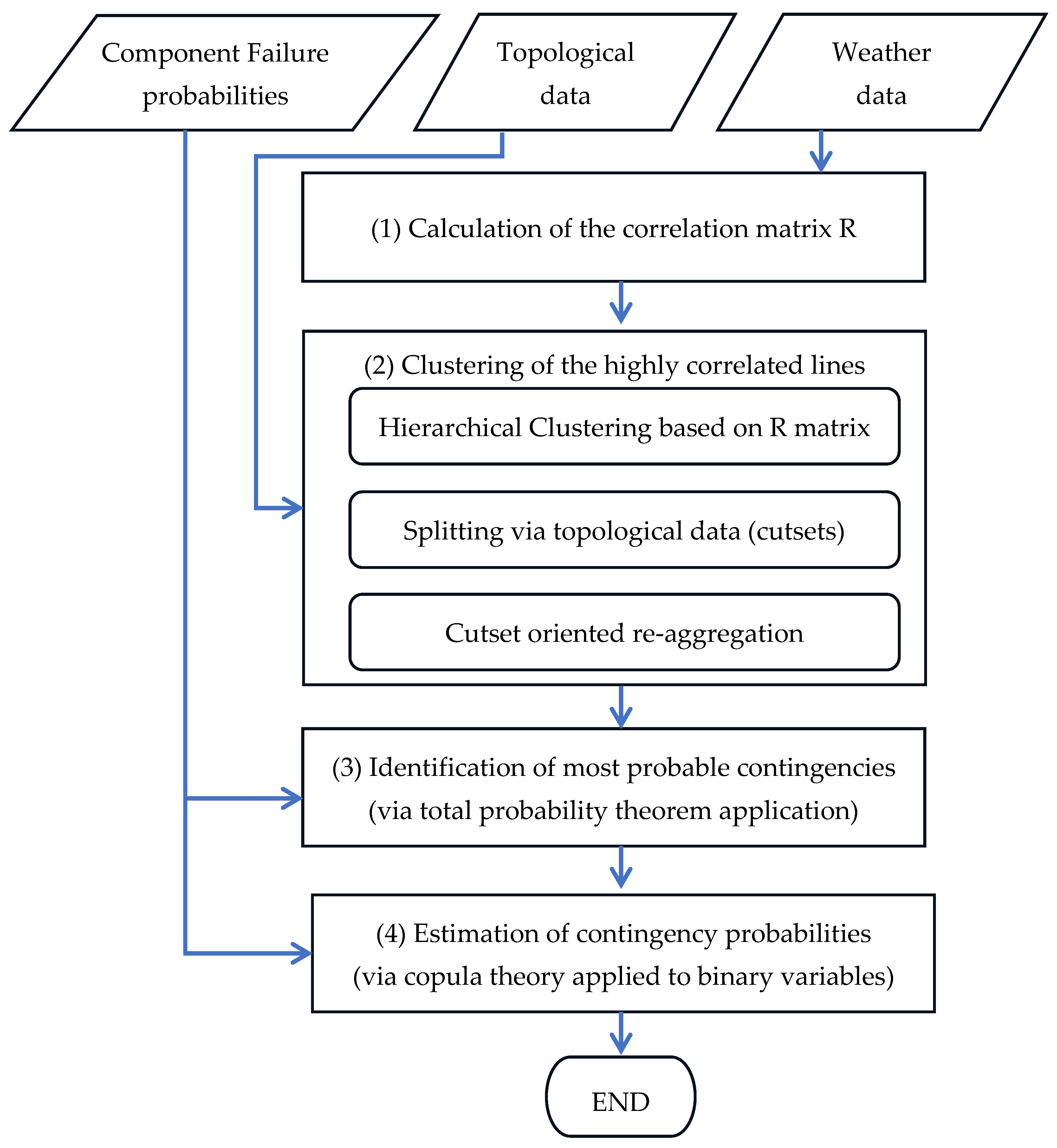
Figure 2 reports the workflow of the proposed methodology for the efficient enumeration of multiple contingencies. It is worth pointing out that the component failure probabilities in input to the process are obtained by combining weather data and infrastructure vulnerability models as recalled in Section 4.1.
3. Clustering of Correlated Lines
This section presents stage 1 (correlation matrix computation) and stage 2 (clustering).
3.1. Calculation of the Correlation Matrix
The starting point for building the correlation matrix is an [Nevents × N] event matrix M evaluated as in (1), where Nevents is the number of relevant weather events and N is the total number of lines considered in the analysis. An event is considered relevant if a specific intensity threshold has been overcome at least for one line.
Matrix M allows to compute the event table, which reports the number of weather events when the intensity threshold has been overcome in the lines, see example referring to lines L1 and L2 in Table 1.
The meaning of the symbols in Table 1 is explained below:
- n11 is the number of severe events for which both lines L1 and L2 are affected by a weather variable exceeding a threshold Th (e.g., in m/s for wind and kg/m for wet snow);
- n10 is the number of severe events for which line L1 is affected while line L2 is not affected by a weather variable exceeding a threshold Th;
- n01 is the number of severe events for which line L2 is affected while line L1 is not affected by a weather variable exceeding a threshold Th;
- n00 is the number of severe events for which neither line is affected by a weather variable exceeding a threshold Th.
The linear correlation coefficient between lines L1 and L2 is computed as in (2).
Repeating the computation in (2) for any pair of lines, the algorithm builds the line correlation matrix R for the whole set of lines, R(i, j) = φij [20].
It is worth noting that the correlation analysis is constrained by the limited availability of data on actual line failures. To address this challenge, the correlation matrix R is constructed by analyzing past weather events. Rather than directly counting component failures, events are identified as critical when the stress placed on the lines by the weather exceeds a predefined threshold based on international and national standards (e.g., 1.5 kg/m for wet snow according to the Italian standard CEI 11.4 [21]). This approach captures potential damage scenarios where lines are more likely to fail together since they are exposed to the same extreme weather conditions.
This approach is general and can also be applied to other natural threats, not necessarily those that are weather-related (e.g., earthquakes), by indicating the lines where a specific intensity threshold of the associated stress variable (e.g., the peak ground acceleration in case of earthquakes) is exceeded for historical events.
3.2. Clustering
The identification of suitable line clusters can significantly improve the efficiency of estimating long-term resilience indicators. As recalled above, clusters are defined as sets of lines such that, within each set, multiple contingencies are likely to occur. Accordingly, the identification of multiple contingencies will be carried out within each cluster, neglecting inter-cluster contingencies.
Clustering leverages dimensionality reduction, which involves a tradeoff between computational speed and accuracy. In fact, as the number of lines within each cluster increases, the required computational time grows exponentially. On the other hand, if the clusters selected are too small, the risk of missing significant multiple contingencies (involving lines from more than one cluster) increases. Therefore, selecting the maximum cluster cardinality, compatible with computational constraints, is essential for achieving both efficiency and accuracy.
Moreover, the correlation matrix R plays a crucial role in this process: it captures the historical impact of weather events on different sets of lines, allowing to choose clusters that optimize this tradeoff. To meet such requirements, the defined clustering algorithm allows to:
- Create clusters with a user-defined threshold of minimum internal correlation between the lines in each cluster;
- Create clusters with a maximum cardinality (NMAX, LI);
- Subdividing clusters that are too large (with cardinality higher than NMAX, LI) into smaller clusters of maximum cardinality NMAX, LI based on topological information.
The steps that compose the algorithm are the following:
- Step 1: identification of the clusters based on the correlation matrix R;
- Step 2: identification of subclusters using topological indications;
- Step 3: aggregation of individual clusters through a mix of topological indications and correlation factors.
3.2.1. Step 1: Clustering of the Lines Based on the Correlation Matrix R
Step 1 applies an agglomerative hierarchical clustering technique [22] to group the lines together based on the correlation matrix R. This technique is chosen because it does not require a predefined number of clusters, which is advantageous in situations where the optimal number of groups is unknown. Additionally, hierarchical clustering allows for easy interpretation of the identified groups.
Two metrics are used in the following steps:
The lines are grouped into clusters using the information of the N × N correlation matrix R:
- The parameters of minimum value of the intra-cluster average correlation () and the distance limit between two distinct clusters () are set;
- The distance matrix between the lines is calculated, defined as D = 1—R’, where R’ is the correlation matrix with all zeros set along the main diagonal and 1 is an N × N matrix entirely filled with ones;
- N groups are defined, each containing one line of the set;
- Lines i and j are identified s.t. D(i, j) = min(min(D));
- Lines i and j are grouped into a new group “N + 1”;
- The cophenetic distance is calculated between the group made up of i and j and the remaining N − 2 groups (excluding the groups related to rows i and j). Ψ is defined as the set of N − 2 groups. This distance is defined as max(max(D([i j], h)));
- The matrix D is updated, in particular D(N + 1, h) and D(h, N + 1) with h ∈ Ψ;
- The rows and columns associated with the original groups i and j are deleted;
- Steps 3 to 7 are repeated until one of the following conditions occurs:
- The minimum value of the intra-cluster mean correlation (calculated as the average value of the linear correlation coefficient between any pair of lines belonging to the same cluster) becomes less than a threshold ;
- The minimum distance between two distinct clusters becomes greater than a threshold .
- Steps 2–9 are repeated on several pairs of parameters , , defined as the Cartesian product of two sets containing reasonable values for both of the aforementioned parameters, in order to select the pair that provides the best performance indicator according to the indications at step 11;
- The pair of parameters that ensures the highest performance index is selected, indicated as the weighted sum of the 5% quantiles of the silhouette coefficient and the internal correlation value of the non-single clusters. This guarantees the best separation between the groups and at the same time a good cohesion within the groups. Values between 0.50 and 0.70 for the silhouette indicate reliable groups, while values between 0.7 and 1 very reliable groups (as they are cohesive and well separated from the others).
3.2.2. Step 2: Splitting of Wide Clusters According to Topological Information (Cutsets)
Step 1 only takes into account the information provided by the correlation matrix: this can lead to clusters with a cardinality (i.e., a number of elements) much greater than the maximum desired value. This problem is addressed in Step 2.
The rationale of this step is to split clusters exceeding a certain size threshold (NMAX, LI) into smaller clusters, making sure that the lines, whose simultaneous tripping causes the disconnection of primary substations, are kept in the same cluster (because such events highly affect resilience indicators such as expected energy not served). This sub-division leverages topological information about the grid to ensure the resulting clusters maintain meaningful relationships between lines.
In particular, the following sub-steps are performed:
- The cutsets of lines that lead to the disconnection of the substations (primary substations, PSs) of the network portion are identified. Then, the connectivity matrix A of dimensions N × NPS is defined where N is the number of lines and NPS is the number of PSs of the considered network, s.t. A(i, j) = 1 if PS j is terminal 1 of line i and A(i, j) = −1 if PS j is terminal 2 of line i, A(i, j) = 0 otherwise;
- For each PS j, a vector Xj of dimensions NPS × 1 is set such that Xj(j) = −1, it is 1 otherwise;
- Yj = A × Xj gives a vector NL × 1 where the non-zero terms represent the minimum subset of lines which cuts PS j;
- For each cluster larger than NMAX, LI:
- The sub-matrix S of matrix A corresponding to the lines belonging to the cluster to be disaggregated is obtained;
- The columns of S are sorted according to the decreasing number of non-zero terms. We obtain the Sord reordered matrix;
- The sub-cluster is identified as the set Lsc of lines associated with the first column of the Sord matrix. The lines of the sub-cluster Lsc are discarded from the lines of the original cluster Lco, redefining the matrix S on the basis of the set Lco’ of the remaining lines to be clustered where card(Lco’) = card(Lco) − card(Lsc), “card” being the “cardinality” operator which indicates the number of elements of the set.
- tems ii and iii are repeated on the new matrix S, updating the set of Lco’ lines to be clustered until the set Lco’ has a cardinality lower than or equal to NMAX, LI;
- The subclusters are reaggregated on the basis of the following criteria:
- The subclusters in pairs form a cutset of the network;
- The sum of the dimensions of the reaggregated subclusters are at most equal to NMAX, LI.
Obviously, at the level of this step it is possible to introduce additional data (e.g., the distance in km between the lines or the proximity of the substations belonging to each sub-cluster), which allows further aggregation of sub-clusters in order to limit the loss of information that this step necessarily entails. Important outcomes of step 2 are the NG clusters and the correlation matrix MR among the NG clusters: this matrix results from the application of steps 1 and 2 to the original correlation matrix R.
3.2.3. Step 3: Cutset-Oriented Re-Aggregation of Clusters
After the first two steps, there are still two aspects to consider:
- There are still some groups composed of a single line that have high correlations with already clustered lines;
- There may be relatively small clusters that can be increased with a small decrease in the intra-cluster correlation.
This step thus has the following two purposes:
- To increase cluster size with little detriment on cluster internal correlation;
- To aggregate unpaired lines with already clustered lines.
Given NG clusters from step 2:
- For each cluster i1 = 1 … NG − 1, the clusters i2 = i1 + 1 …. NG are analyzed and the following are calculated:
- The mean value of the correlation between each pair of clusters i1 and i2 (defined as the arithmetic mean of the absolute values of the linear correlation coefficients, each calculated on a different pair of lines, one belonging to cluster i1 and the other to cluster i2) reported in position (i, j) of matrix MR;
- The maximum value of the correlation between two lines of clusters, i1 and i2;
- The best candidates for aggregation between clusters are identified according to the following criteria:
- Clusters that fully define a cutset (topological clusters) and have an average inter-cluster correlation at least equal to a fixed value ;
- Clusters that have an inter-cluster correlation no less than a fixed value ;
- Topological clusters that have a maximum correlation value at least equal to a fixed value equal to .
- Two matrices, M1 and M2, of dimension NG × NG are defined s.t. in position (i, j) if they contain 1 or 0, respectively, depending on whether the following criteria are verified or not:
- criterion c.i or c.ii for matrix M1;
- criterion c.iii for matrix M2.
- The conditionality matrix MC between clusters i1 and i2 is also defined such that MC(i1, i2) = 0 if the sum of the dimensions of clusters i1 and i2 is greater than a defined value (parameter NMAX, LI); it is 0 otherwise;
- For the candidates selected in point 1.c, the Matrix_total of the performance indicators is calculated as in (3):where α is the weight given to the cutset-based topological clustering;
- The previous steps 1 and 2 are repeated until:
- the residual correlation between the “single” groups and the multi-line groups does not fall below an established threshold (), or;
- the maximum number of iterations is exceeded.
3.3. Management of Greenfield Lines and Partially Buried Lines
The clustering approach so far presented relies on historical data describing the stress of past weather events on grid assets. It may be required to adopt the methodology to the scenario of new lines in the planning stage (green field lines), for which similar historical data are not available, and to the scenario of the partial burying of existing lines, which would prevent the buried portions of lines from being affected by the wet snow weather threat.
To this aim, considering the planning intervention as accomplished, the steps of the re-clusterization with Npi partially buried lines and Ngreen greenfield lines are shown below:
- Consider the clusters Ch h = 1 … NC identified in the pre-intervention analysis;
- Modify matrix M in the columns of the partially buried lines q = 1 … Npi;
- The partially buried lines that are part of singleton clusters in the pre-intervention analysis remain in the singleton cluster;
- Increase the number of matrix M columns by adding the columns of greenfield lines i = 1 … Ngreen (on the basis of the hypothetical layout of the greenfield lines, the events of exceeding the threshold in the greenfield lines are counted considering the same weather events of the pre-intervention analysis);
- Calculate the correlation coefficients Rqj between each partially buried line q = 1 … Npi not belonging to singleton clusters and the other lines j;
- Calculate the correlation coefficients Rij between the greenfield line i = 1 … Ngreen and the other lines j;
- Greenfield line i is attributed to cluster h*, which has the highest median value calculated on the absolute values of the coefficients Ris with s ∈ Ch, i.e., ;
- Steps 6 and 7 are repeated for all greenfield lines.
In order to assure the consistency of the risk indicators before and after the application of the specific resilience enhancement measure (i.e., the addition of a greenfield line or the burying of a line), the new combinations involving greenfield lines and existing lines are not subject to the minimum threshold ε normally applied to contingency probability and described in Section 4.3, while combinations involving partially buried lines are subject to the minimum probability threshold ε.
4. Selection of Contingencies and Probability Computation
While selecting clusters with a limited number of lines (i.e., line cardinality) helps control the combinatorial explosion, analyzing all possible combinations of line failures within even these smaller clusters (typically 10–15 lines) still represents a computationally tough task.
This section presents an effective methodology based on the total probability theorem and copulas of binary variables to efficiently filter out multiple contingencies that is also suitable for large power system applications. With reference to Section 2.3, this section describes stage 3 (cluster-based contingency identification) and stage 4 (contingency probability calculation) of the methodology.
Three steps compose the algorithm for contingency probability calculation and contingency selection:
- Computation of the probability of the “AND” event of multiple line trippings;
- Iterative filtering based on total probability theorem;
- Calculation of the probability of occurrence of retained contingencies.
A preliminary discussion on the probability modeling of multiple contingencies is proposed in the following.
4.1. Probabilistic Modeling of Multiple Contingencies
The evaluation of the probability of multiple contingencies is based on the analysis of historical data series related to past weather events: for recorded past events, the goal of such analysis is to identify the set of affected lines during the time interval (typically a few hours) when grid assets were exposed to the weather event. These data must be processed in a proper way to identify the actual multiple failure events and their probabilities in the chosen time interval (e.g., one hour).
On an hourly basis, it is also possible to assume the mutual exclusivity of the contingencies (due to the reduced time interval considered). Therefore, the following condition holds: the hourly probability of a line failure must be equal to the sum of the hourly probabilities of the contingencies that foresee the failure of that line.
For illustrative purposes, consider Figure 3: in case (a), two single failure events occur involving lines L1 and L2 in different periods of year Y (February and March), while in case (b), a contingency N-2 occurs, involving lines L1 and L2, during the same weather event in February. For the purposes of calculating the resilience indicators, it is of interest to evaluate the probability of the multiple events as in case (b). To do this, it is necessary to assess the probability of failure focusing on a limited time interval (for example, one hour). In fact, if the probabilities of the combinations of events were calculated starting from the annual probabilities of line failure, the combinations would be evaluated on an “annual basis” including situations analogous to case (a), i.e., considering as multiple contingencies all the sets of single trips that occurred in the course of the year under analysis. Conversely, focusing on the average hourly probability of failure allows to evaluate the probability of “real” multiple contingencies, i.e., those that comprise the simultaneous loss (due to the same weather event) of several network components, as in case (b).
The hourly failure probability of a line can be estimated using its annual failure return period, obtained through the extreme value analysis of historical or prospective weather data. This estimation assumes an underlying exponential distribution with a constant, year-averaged failure rate (λ): this is a reasonable assumption for long-term studies. So, the average hourly probability of the failure of a generic line j, Pj,1hr, is given by (4).
where represents the annual probability of failure of generic line j, i.e., the inverse of the return period (RP) of failure of the line. The value of is obtained by combining the line vulnerability model with the probabilistic model of the weather threat variables [1,13,20].
Historical weather data, along with the average hourly failure probabilities (P1hr) for each line, estimated using weather data and vulnerability models, is then used to derive the average hourly probabilities of various contingencies, as described in the following.
In the sequel, a contingency is meant as a combination (AND event) of line trippings and non trippings due to the threat actions, occurring within a defined time interval of analysis (e.g., one hour).
4.2. Copula-Based Computation of Contingency Probability
The mathematical formulation employed for the probability calculation relies on copulas [25]. Copulas are versatile in describing complex dependences among random variables compared to alternative methods such as conditional distributions. This characteristic makes them well suited for this application, where the relationships between the variables might not be straightforward. A specific copula-based formulation is used to calculate probabilities and a specific computational algorithm is employed for evaluation as described in the following.
Let us define two types of events:
Fj = {line Lj tripping due to initiating event};
Tj = {overcoming of a critical weather variable threshold at line Lj}.
Some reasonable assumptions are proposed in (5).
Under these assumptions, it is possible to derive the expression in (6) to compute the probability of the AND event related to the failures of n lines:
Two terms are kept separate in (6), i.e., the failure probabilities of the lines and the correlation of the weather event on the n lines given by ratio . Under the assumption that the correlation of line failures can be assimilated to the correlation of events of weather threshold exceedance on the same lines, Equation (6) can be modeled using the copula theory as follows.
Each line L is associated with a binary variable X such that X = 0 when the line is in service and X = 1 when the line is failed (failure event F).
Therefore, a Bernoulli probability mass function (pmf) can be associated to the variable X so that conditions in (7) are fulfilled:
where P(Fj) is the probability of a failure in the j-th line. In the sequel, for the sake of brevity the following notation is used: P(Fj) = pj.
With a copula-based notation, the probability of the AND event of line failures in (6) can be computed as the copula cumulative distribution function (CDF) evaluated at pi values, considering a suitable copula family. Different family copulas have been tested (e.g., empirical, Clayton and Frank copulas), and we have found that the Gaussian copula is the best tradeoff between accuracy and computational speed for a reliable evaluation of the multiple contingency probabilities.
The numerical computation of the copula CDF represents an important topic in recent research [26,27] because the accuracy of such computation can decrease rapidly when the dimensions of the copula, i.e., the number of involved variables, increases. Specifically, for applications to realistic power systems, one can find line clusters with cardinalities in the range of 10–20, which can jeopardize the accuracy of commonly used algorithms, such the one described in [26]. Thus, making the methodology suitable for applications to real power systems requires the adoption of more recent techniques. Specifically, the proposed methodology exploits Botev’s tilting method [27] to accurate evaluate the copula CDF.
4.3. Filtering of Failure Combinations Based on Total Probability Theorem
The calculation of CDF values via copulas allows to filter out contingencies with negligible probability by exploiting the total probability theorem [25]. In particular, it efficiently evaluates the probabilities of an exhaustive set of failure combinations (logic AND) via the copula formulation (Section 4.2) and discards the combinations for which the probability is lower than a given probability threshold. As the h-th contingency consists of a combination of n_th trippings and n_nth not trippings, its probability is always lower than the probability of the AND of the n_th trippings thanks to the total probability theorem. Thus, the contingencies that include any of the discarded AND combinations are also discarded by the algorithm.
4.4. Calculation of the Probability of Occurrence of Multiple Contingencies
Once the clusters of lines and, within each of the clusters, the sets of line trippings with the most significant probabilities have been identified (stage 3 of the process outlined in Section 2.3), it is possible to evaluate the probability of the combinations of line trippings and not trippings (i.e., contingency probability) by applying the theory of copulas for binary variables [25] in each cluster (stage 4).
Using Sklar’s theorem applied to discrete (particularly binary) variables, the probability of the occurrence of a given set St of trippings and a set Snt of not-trippings, i.e., P(St and Snt), can be written as an algebraic sum of the cumulative distribution of probability of the copula C (copula CDF) evaluated at suitable points according to the general formula indicated in (8).
where and in (9) is a vector with q components s1, …, sq, where sj can be xj or xj − 1.
In case of more clusters, the methodology assumes independence among failures affecting lines belonging to different clusters.
Once the average hourly probabilities of occurrence of the contingencies have been calculated, their annual probabilities are obtained assuming that we are dealing with (independent) Poissonian events with the calculated hourly rate. In particular, the annual probability of the generic h-th contingency Pctg h, 1yr is a function of the hourly probability of the same h-th contingency Pctg h, 1hr by means of (10).
where T = 8760 is the number of hours in a year. The expression in (10) represents the probability that the h-th contingency, modeled as a Poisson event, occurs at least once during the year.
5. Case Study
5.1. Test System and Simulations
To validate its effectiveness in real-world applications, the proposed methodology was applied to a detailed model encompassing a portion of the Italian extra-high-voltage (EHV) transmission system.
The analysis considered the threat of wet snow and encompassed all 647 EHV and high voltage (HV) overhead lines (OHLs) within the selected area. Details of the simulations conducted are provided in Table 2.
5.2. Simulation CLU: Line Clustering for Wet Snow Events
Figure 4a shows the size of the identified clusters (top left) and their level of internal correlation (defined as the average value of the absolute values of the correlation coefficients between distinct elements from the same cluster and reported in the bottom left diagram) after stage 1. Figure 4b shows the analogous results after stage 3.
It is worth noting that after stage 1 the internal correlation among the lines in the clusters is very high (lowest value is 0.7) but the cardinality of many clusters can be larger than 60. After stage 1, the silhouette coefficients for groups with more than one element mostly show values between 0.5 and 1, which demonstrates the correctness of the clustering of the large majority of the lines inside each cluster. To this purpose, Table 3 shows the quantiles for the silhouette index distribution over all the lines subject to clusterization: 75% of all the lines have a silhouette index higher than 68% after stage 1.
After leveraging grid topology and merging smaller clusters, the resulting clusters hold a maximum of NMAX, LI lines each. Importantly, these clusters still exhibit a strong internal connection between lines, with a minimum correlation value of around 0.5.
Many clusters identified by the algorithm correspond to sets of lines that had failed at the same time during past weather events and that are already known by the TSO as “responsible for multiple contingencies” and often for energy not supplied to the utilities.
Table 4 reports the internal correlation for the lines inside the topological cutsets. It is also worth noting that most of the topological cutsets preserve a significant internal correlation (50% of the topological cutsets have an internal correlation value higher than 50%).
Table 5 reports the quantiles of the distribution of the average values of the internal correlation of the clusters.
It is worth noting that the internal correlation exceeds 0.52 in 95% of the clusters and that the median value is very high (0.78).
5.3. Simulation PRO: Tests on the Algorithm for Contingency Probability Computation
This simulation case assesses the performances (in terms of accuracy and speed) of the algorithm to compute the copula CDF values used to assess contingency probabilities.
In particular, a typical necessary condition that must be satisfied on an hourly basis to assess the algorithm accuracy is in (11), i.e., the sum of the hourly probability of contingencies involving line j should be equal to the hourly failure probability of line j.
where PCTG,i is the hourly probability of i-th contingency involving line j and is the number of contingencies involving line j. The metrics used to assess the fulfillment of such a condition is the percentual error in (12) between the line failure probability derived from the failure return periods RPj, i.e., and the reconstructed failure probability .
This metric is computed for each line of one cluster from the set within simulation CLU considering two alternative methods mentioned in Section 4.3:
The same metric is computed for:
- Different numbers of lines in the cluster, with the same correlation matrix R;
- Different values for the return periods, with the same cluster cardinality and matrix R;
- Different correlation matrices R among the lines, with the same line cardinality.
The original cluster has 12 lines, with the failure return periods reported in Table 6 for subcases (a), (b) and (c). The large dispersion of RP values adopted in the simulation reflects a typical condition found during power system resilience analyses.
Subcases (a) and (b) are run considering a very high correlation (>0.9) among all the lines in the cluster: this is a common condition due to the fact that the previous stages of the methodology create clusters with high internal correlations.
5.3.1. Subcase (a): Comparison of the Two Algorithms with Different Line Cardinalities
This subcase is run considering the RP values in the first row of Table 6 and a very high correlation among all the lines of the cluster. Table 7 reports the percentage error for cluster cardinalities {5, 7, 10, 12} for the two algorithms. It is worth noting that algorithm A maintains acceptable errors below 15% only for the lowest cardinalities (5 and 7) but the error becomes unacceptable for higher cardinalities.
Figure 5 reports the percentual errors on the hourly failure probabilities for the 12 lines of the cluster using algorithm A (left) and algorithm B (right).
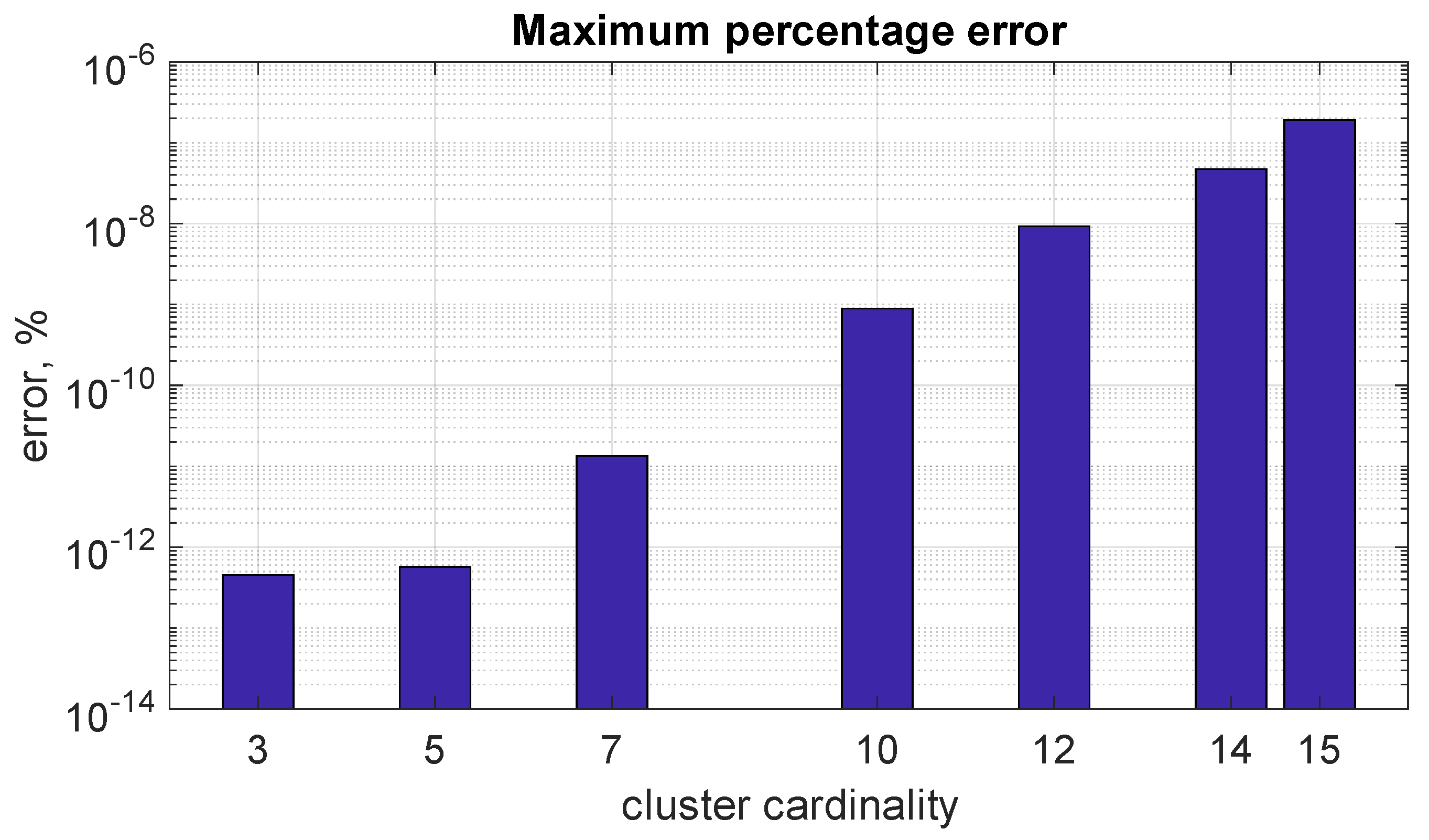
Figure 6 reports the maximum percentual errors over the lines using algorithm B for different cardinalities of the cluster. The percentual errors are also very low for a significant number of lines in the cluster (up to 15). From Table 7, it can be seen that algorithm A attains maximum errors equal to 10.5% and 413.5% for the same 7-line and 10-line clusters, respectively.
5.3.2. Subcase (b): Comparison of the Two Algorithms with Different RP Values
A cluster with the first 12 lines of Table 6 is used in the present subcase, but three RP values are changed in order to quantify the potential changes in the performances (accuracy and computational efficiency) of the two algorithms.
Table 8 also presents the computational times for the two algorithms A and B and for two cardinalities of the cluster (10 and 12, a typical limit value for the cluster cardinality representing a good tradeoff between computational burden and accuracy during the clusterization process).
It is important to note that the error given by algorithm A is much more sensitive to the values of RP (passing from 413% in subcase (a) to 228% for the 10-line cluster), while algorithm B is extremely accurate and its accuracy does not depend on the RP values. Algorithm A errors remain unacceptable for cluster cardinalities higher than 5–7.
Table 9 further compares the computational times of algorithms A and B for clustering line sets of different sizes (10 and 12 lines). Notably, a key advantage of algorithm B emerges: its speedup factor over algorithm A increases for clusters with higher cardinalities. This is crucial for resilience analysis in large power systems, as CLU simulations often identify clusters with high numbers of lines. Furthermore, the computational time for algorithm B is much less sensitive to the RP values; in fact, it takes 175 s and 38 s for the 12-line and 10-line clusters in subcase (a). In contrast, the computational time for algorithm A has a high dependency on the RP values: for the 12-line cluster, it takes 816s against 1067s in subcase (a). If one considers a cluster of 15 lines, algorithm B takes 2040 s, against more than 4 h for algorithm A.
5.3.3. Subcase (c): Comparison of the Two Algorithms with Different Correlation Levels
This test is meant to understand the impact of the level of internal correlation among the lines of the cluster on the accuracy of the probability computation algorithm.
Table 10 shows the maximum percentual errors in absolute value among the lines of a cluster with a cardinality of eight for four correlation levels.
It is worth noting that algorithm A improves its accuracy when the correlation level is reduced but algorithm B is still much more accurate than algorithm A, even for relatively lower correlations, keeping the maximum error below 0.5% for any analyzed correlation level. Moreover, given the same correlation matrix, the computational time for algorithm B is much smaller than algorithm A in the large majority of the simulated cases.
5.3.4. Some Remarks
These results show that algorithm B, based on Botev’s tilting method, emerges as the clear winner with respect to:
- Enhanced speed and accuracy: compared to algorithm A, Botev’s algorithm boasts significantly faster execution times and demonstrably higher accuracy, at least for contingency probability computations in power system resilience assessment. This improved accuracy is particularly crucial, as even small deviations in contingency probabilities can have substantial consequences.
- Robustness across scenarios: algorithm B exhibits remarkable stability to various input characteristics. Its calculation time remains independent of the specific line failure probabilities within a cluster, unlike algorithm A, which can be sensitive to these values. This robustness ensures reliable performance across diverse situations.
- Accuracy maintained for large clusters: even when dealing with very large clusters (tested up to a size of 15, often considered the upper limit) and significant variations in line reliability parameters (RPs), algorithm B delivers exceptional accuracy. This characteristic makes it ideal for real-world power system analysis, where large clusters and diverse RP values are common.
- Adaptability to correlation matrices: Botev’s algorithm maintains its high accuracy regardless of the correlation matrix configuration. It performs equally well with highly correlated, moderately correlated, or weakly correlated line failures, providing a versatile solution for various power system scenarios.
By virtue of these advantages, algorithm B establishes itself as the most robust and accurate choice for calculating multivariate Gaussian CDFs in contingency probability assessments. This superiority has led to its adoption in the proposed methodology, guaranteeing a solid foundation for precise multiple contingency probability evaluation, a crucial aspect of power system resilience analysis.
6. Conclusions
The paper has proposed a methodology for an efficient selection of the most relevant multiple contingencies to be considered in resilience studies. Specifically, this methodology has been conceived to ensure scalability and efficiency in its application to realistic models of large power systems.
To attain these goals, the methodology quantifies the correlation among the weather events affecting the lines of the grid by computing a correlation matrix (R) from historical events. It then utilizes an innovative three-step clustering process to identify groups of lines likely to trip together. This clustering leverages information from both the correlation matrix and the grid’s topology.
This approach allows avoiding the potential combinatorial explosions deriving from the brute enumeration of all the N-k potential contingencies on the whole set of branches in real-world power systems.
The simulations performed on a portion of the Italian EHV grid show the effectiveness of the proposed clustering process in aggregating lines that are more likely to fail together and the ability to fast screen the contingencies inside each cluster. In particular, many identified clusters contain sets of lines that have historically failed together, known by system operators (TSOs) as “responsible for multiple contingencies” and often leading to energy not served to customers.
Additionally, simulations show that the use of Botev’s tilting algorithm to compute Gaussian multivariate in the copula-based calculation of contingency probability is accurate and fast even for relatively large line clusters, providing multiple contingency probabilities that are consistent with the line failure probabilities. This makes the proposed approach a sound solution for resilience analyses in real-world power systems.
Further developments will concern the extension of the methodology to multiple threats, as well as the modeling of the perspective evolution of correlations over the future decades.
Author Contributions
Conceptualization, E.C., D.C.; methodology, E.C., A.P.; software, A.P.; validation, E.C.; writing—original draft preparation, A.P.; writing—review and editing, E.C., D.C.; supervision, E.C. All authors have read and agreed to the published version of the manuscript.
Funding
This work was financed by the Research Fund for the Italian Electrical System under the Three-Year Research Plan 2022–2024 (DM MITE n. 337, 15 September 2022), in compliance with the Decree of 16 April 2018.
Data Availability Statement
Data that support the presented findings are not publicly available due to confidentiality issues concerning National Transmission Grid.
Conflicts of Interest
Authors Emanuele Ciapessoni, Diego Cirio and Andrea Pitto were employed by the company Ricerca sul Sistema Energetico—RSE S.p.A. The authors declare that the research was conducted in the absence of any commercial or financial relationships that could be construed as a potential conflict of interest.
References
- Billinton, R.; Li, W. Reliability Assessment of Electric Power Systems Using Monte Carlo Methods; Plenum Press: New York, NY, USA, 1994. [Google Scholar]
- Panteli, M.; Mancarella, P. Influence of extreme weather and climate change on the resilience of power systems: Impacts and possible mitigation strategies. Electr. Power Syst. Res. 2015, 127, 259–270. [Google Scholar] [CrossRef]
- Zhang, D.; Li, C.; Goh, H.H.; Ahmad, T.; Zhu, H.; Liu, H.; Wu, T. A comprehensive overview of modeling approaches and optimal control strategies for cyber-physical resilience in power systems. Renew. Energy 2022, 189, 1383–1406. [Google Scholar] [CrossRef]
- Paul, S.; Poudyal, A.; Poudel, S.; Dubey, A.; Wang, Z. Resilience assessment and planning in power distribution systems: Past and future considerations. Renew. Sustain. Energy Rev. 2024, 189, 113991. [Google Scholar] [CrossRef]
- Kjølle, G.H.; Gjerde, O. The OPAL Methodology for Reliability Analysis of Power Systems; Technical Report; SINTEF Energy Research: Trondheim, Norway, 2012. [Google Scholar]
- Lieber, D.; Nemirovskii, A.; Rubinstein, R.Y. A fast Monte Carlo method for evaluating reliability indexes. IEEE Trans. Reliab. 1999, 48, 256–261. [Google Scholar] [CrossRef]
- Cervan, D.; Coronado, A.M.; Luyo, J.E. Cluster-based stratified sampling for fast reliability evaluation of composite power systems based on sequential Monte Carlo simulation. Int. J. Electr. Power Energy Syst. 2023, 147, 108813. [Google Scholar] [CrossRef]
- González-Fernández, R.A.; Leite da Silva, A.M.; Resende, L.C.; Schilling, M.T. Composite Systems Reliability Evaluation Based on Monte Carlo Simulation and Cross-Entropy Methods. IEEE Trans. Power Syst. 2013, 28, 4598–4606. [Google Scholar] [CrossRef]
- Hua, B.; Bie, Z.; Au, S.-K.; Li, W.; Wang, X. Extracting Rare Failure Events in Composite System Reliability Evaluation Via Subset Simulation. IEEE Trans. Power Syst. 2015, 30, 753–762. [Google Scholar] [CrossRef]
- Zhao, Y.; Han, Y.; Liu, Y.; Xie, K.; Li, W.; Yu, J. Cross-Entropy-Based Composite System Reliability Evaluation Using Subset Simulation and Minimum Computational Burden Criterion. IEEE Trans. Power Syst. 2021, 36, 5189–5209. [Google Scholar] [CrossRef]
- Liu, Y.; Singh, C. Reliability evaluation of composite power systems using markov cut-set method. IEEE Trans. Power Syst. 2010, 25, 777–785. [Google Scholar] [CrossRef]
- Wang, M.; Xiang, Y.; Wang, L. Identification of critical contingencies using solution space pruning and intelligent search. Electr. Power Syst. Res. 2017, 149, 220–229. [Google Scholar] [CrossRef]
- Ciapessoni, E.; Cirio, D.; Pitto, A.; Pirovano, G.; Faggian, P.; Marzullo, F.; Lazzarini, A.; Falorni, F.; Scavo, F. A methodology for resilience oriented planning in the Italian transmission system. In Proceedings of the 2021 AEIT International Annual Conference (AEIT), Catania, Italy, 4–8 October 2021; pp. 1–6. [Google Scholar]
- Faustino Agreira, C.I.; Machado Ferreira, C.M.; Maciel Barbosa, F.P. Electric Power System Multiple Contingencies Analysis Using the Rough Set Theory. In Proceedings of the UPEC 2003 Conference, Thessalonica, Greece, 1–3 September 2003. [Google Scholar]
- Eppstein, M.J.; Hines, P.D.H. A “Random Chemistry” Algorithm for Identifying Collections of Multiple Contingencies That Initiate Cascading Failure. IEEE Trans. Power Syst. 2012, 27, 1698–1705. [Google Scholar] [CrossRef]
- Lesieutre, B.; Roy, S.; Donde, V.; Pinar, A. Power System Extreme Event Screening using Graph Partitioning. In Proceedings of the North American Power Symposium, Carbondale, IL, USA, 17–19 September 2006. [Google Scholar]
- Kiel, E.S.; Kjølle, G.H. A Monte Carlo sampling procedure for rare events applied to power system reliability analysis. In Proceedings of the 2023 IEEE PES Innovative Smart Grid Technologies Europe (ISGT EUROPE), Grenoble, France, 23–26 October 2023; pp. 1–5. [Google Scholar]
- Ciapessoni, E.; Cirio, D.; Pitto, A.; Van Harte, M.; Panteli, M.; Mak, C. Defining power system resilience. Electra CIGRE J. 2019, 316, 1–3. [Google Scholar]
- Ciapessoni, E.; Cirio, D.; Pitto, A.; Sforna, M. Quantification of the Benefits for Power System of Resilience Boosting Measures. Appl. Sci. 2020, 10, 5402. [Google Scholar] [CrossRef]
- Ciapessoni, E.; Cirio, D.; Ferrario, E.; Lacavalla, M.; Marcacci, P.; Pirovano, G.; Pitto, A.; Marzullo, F.; Falorni, F.; Scavo, F.; et al. Validation and application of the methodology to compute resilience indicators in the Italian EHV transmission system. In Proceedings of the 2022 CIGRE Session, Paris, France, 28 August–2 September 2022; pp. 1–14. [Google Scholar]
- CEI (Italian Electrotechnical Committee). Norme Tecniche per la Costruzione di Linee Elettriche Aeree Esterne; CEI 11-4; CEI Press: Milan, Italy, 1998. (In Italian) [Google Scholar]
- Maimon, O.; Rokach, L. Clustering methods. In Data Mining and Knowledge Discovery Handbook; Springer: Berlin/Heidelberg, Germany, 2006; pp. 321–352. [Google Scholar]
- Saraçli, S.; Dogan, N.; Dogan, I. Comparison of hierarchical cluster analysis methods by cophenetic correlation. J. Inequalities Appl. 2013, 2013, 203. [Google Scholar] [CrossRef]
- Kaufman, L.; Rousseeuw, P. Finding Groups. In Data: An Introduction to Cluster Analysis; John Wiley & Sons: Hoboken, NJ, USA, 1990. [Google Scholar]
- Nelsen, R.B. An Introduction to Copulas; Springer: New York, NY, USA, 2006. [Google Scholar]
- Genz, A. Numerical Computation of Rectangular Bivariate and Trivariate Normal and t Probabilities. Stat. Comput. 2004, 14, 251–260. [Google Scholar] [CrossRef]
- Botev, Z.I. The Normal Law Under Linear Restrictions: Simulation and Estimation via Minimax Tilting. J. R. Stat. Soc. 2017, 79, 125–148. [Google Scholar] [CrossRef]
Figure 1.
Bowtie conceptual scheme of the RELIEF risk-based resilience assessment framework [19].
Figure 1.
Bowtie conceptual scheme of the RELIEF risk-based resilience assessment framework [19].

Figure 2.
Workflow of the proposed methodology for the efficient enumeration of multiple contingencies for resilience analyses.
Figure 2.
Workflow of the proposed methodology for the efficient enumeration of multiple contingencies for resilience analyses.

Figure 3.
Difference between (a) two failures occurring at different time instants over the year and (b) a N-2 contingency.
Figure 3.
Difference between (a) two failures occurring at different time instants over the year and (b) a N-2 contingency.

Figure 4.
Main results after stage 1 (a) and after stage 3 (b): size of the clusters (top left) and level of intra-c luster correlation (bottom left).
Figure 4.
Main results after stage 1 (a) and after stage 3 (b): size of the clusters (top left) and level of intra-c luster correlation (bottom left).

Figure 5.
Percentual errors on the line failure probabilities for a cluster with cardinality equal to 12 using algorithm A (a) and algorithm B (b).
Figure 5.
Percentual errors on the line failure probabilities for a cluster with cardinality equal to 12 using algorithm A (a) and algorithm B (b).

Figure 6.
Percentual errors versus number of clustered lines—algorithm B.


Table 1.
Event table for lines L1 and L2.
| L2 | Not L2 | Totals | |
|---|---|---|---|
| L1 | n11 | n10 | n1* |
| not L1 | n01 | n00 | n0* |
| Totals | n*1 | n*0 |
Table 2.
Summary of the simulation cases.
| Sim ID | Description | Goal |
|---|---|---|
| CLU | Three-step clustering algorithm application to the set of 647 lines, assuming a maximum cardinality NMAX, LI = 12. | To verify the representativeness of the identified clusters with respect to historical weather events. |
| PRO | Copula-based algorithm application via two alternative algorithms to one specific cluster of the line set analyzed in sim CLU. | To verify the accuracy and the robustness in the copula CDF computation method adopted in the methodology. |
Table 3.
Quantiles of the silhouette index distribution for the lines subject to clusterization.
| Probability | 0.05 | 0.25 | 0.5 | 0.75 | 0.95 |
| Quantile | 0.2176 | 0.6806 | 0.9671 | 1.0000 | 1.0000 |
Table 4.
Quantiles of the distribution of mean values of the internal correlation of the topological cutsets.
Table 4.
Quantiles of the distribution of mean values of the internal correlation of the topological cutsets.
| Probability | 0.05 | 0.25 | 0.5 | 0.75 | 0.95 |
| Quantile | 0.3162 | 0.4709 | 0.6005 | 0.7857 | 0.9901 |
Table 5.
Quantiles of the distribution of mean values of the internal correlation of the clusters.
| Probability | 0.05 | 0.25 | 0.5 | 0.75 | 0.95 |
| Quantile | 0.5272 | 0.6583 | 0.7826 | 0.9901 | 0.9901 |
Table 6.
Parameters used for the simulations in the subcases (a)–(c).
| Subcase | Set of RPs (Year) | Cluster Cardinality | Minimum Correlation in the Cluster |
|---|---|---|---|
| (a) | 22, 2743, 32, 33, 38, 46, 959, 1374, 150, 150, 10, 72, 400, 90, 120 | 5, 7, 10, 12, 14, 15 | >0.9 |
| (b) | 22, 100(*), 32, 33, 38, 46,959, 1374, 50(*), 50(*), 10, 72, 400, 90, 120 | 10, 12 | >0.9 |
| (c) | Same as subcase (a) | 12 | >0.9, 0.8, 0.5, 0.3 |
(*) different values between subcases (a)–(c) and subcase (b).
Table 7.
Comparison of maximum percentage error—algorithms A and B, subcase (a).
| Maximum Percentage Error (%) | Computational Time (s) | |||
|---|---|---|---|---|
| Cluster Cardinality | Algorithm A | Algorithm B | Algorithm A | Algorithm B |
| 3 | 4.43 × 10⁻¹³ | 4.51 × 10⁻¹³ | 0.9 | 1.5 |
| 5 | 3.2 | 5.72 × 10⁻¹³ | 3.6 | 2.7 |
| 7 | 10.5 | 1.35 × 10⁻¹¹ | 16 | 5.8 |
| 10 | 413.5 | 8.93 × 10⁻¹⁰ | 217.9 | 38 |
| 12 | 1945 | 9.30 × 10⁻⁹ | 1067 | 175 |
Table 8.
Comparison of maximum percentage error—algorithms A and B, subcase (b).
| Maximum Percentage Error (%) | ||
|---|---|---|
| Cluster Cardinality | Algorithm A | Algorithm B |
| 10 | 228 | 2.41 × 10⁻¹⁰ |
| 12 | 1430 | 2.75 × 10⁻⁸ |
Table 9.
Comparison of computational performance—algorithms A and B, subcase (b).
| Computational Time (s) | Speed up Ratio | ||
|---|---|---|---|
| Cluster Cardinality | Algorithm A | Algorithm B | |
| 10 | 164 | 38 | 4.3 |
| 12 | 816 | 175 | 4.7 |
Table 10.
Maximum percentual errors with different correlation levels—algorithms A and B, subcase (c).
Table 10.
Maximum percentual errors with different correlation levels—algorithms A and B, subcase (c).
| Correlation Level | Algorithm A, % | Algorithm B, % | ||
|---|---|---|---|---|
| Maximum Percentual Error, % | Computational Time, s | Maximum Percentual Error, % | Computational Time, s | |
| Very high (min corr > 0.9) | 41.7 | 40.0 | 6.91 × 10⁻¹¹ | 9.9 |
| High (min 0.8) | 59.5 | 35.0 | 0.21 | 10.0 |
| Medium (min 0.5) | 22.2 | 12.3 | 0.03 | 10.1 |
| Low (min 0.3) | 4.0 | 8.2 | 2.86 × 10⁻³ | 10.1 |
Disclaimer/Publisher’s Note: The statements, opinions and data contained in all publications are solely those of the individual author(s) and contributor(s) and not of MDPI and/or the editor(s). MDPI and/or the editor(s) disclaim responsibility for any injury to people or property resulting from any ideas, methods, instructions or products referred to in the content. |
© 2024 by the authors. Licensee MDPI, Basel, Switzerland. This article is an open access article distributed under the terms and conditions of the Creative Commons Attribution (CC BY) license (https://creativecommons.org/licenses/by/4.0/).
Share and Cite
MDPI and ACS Style
Ciapessoni, E.; Cirio, D.; Pitto, A. An Efficient Methodology to Identify Relevant Multiple Contingencies and Their Probability for Long-Term Resilience Studies. Energies 2024, 17, 2028. https://0-doi-org.brum.beds.ac.uk/10.3390/en17092028
AMA Style
Ciapessoni E, Cirio D, Pitto A. An Efficient Methodology to Identify Relevant Multiple Contingencies and Their Probability for Long-Term Resilience Studies. Energies. 2024; 17(9):2028. https://0-doi-org.brum.beds.ac.uk/10.3390/en17092028
Chicago/Turabian StyleCiapessoni, Emanuele, Diego Cirio, and Andrea Pitto. 2024. "An Efficient Methodology to Identify Relevant Multiple Contingencies and Their Probability for Long-Term Resilience Studies" Energies 17, no. 9: 2028. https://0-doi-org.brum.beds.ac.uk/10.3390/en17092028
Note that from the first issue of 2016, this journal uses article numbers instead of page numbers. See further details here.