The Impact of System Sizing and Water Temperature on the Thermal Characteristics of Floating Photovoltaic Systems

Abstract

Accurately calculating the annual yield of floating PV (FPV) systems necessitates incorporating appropriate FPV-specific heat loss coefficients into the calculation, including both wind-dependent and wind-independent factors. The thermal behavior of several FPV systems has been investigated within this study, through the analysis of heat loss coefficients across various system sizes and configurations. Over a one-year period, data were collected from two measurement sites with three distinct systems: two ~50 kWp demonstrator-scale setups of Solarisfloat (azimuthal tracking) and Solar Float (East-West orientation) and a 2 MWp commercial-scale East–West system by Groenleven. The Solarisfloat demonstrator revealed a wind-dependent heat loss coefficient of 3.2 W/m³Ks. In comparison, the Solar Float demonstrator system displayed elevated wind-dependent heat loss coefficients, measuring 4.0 W/m³Ks for the east-facing module and 5.1 W/m³Ks for the west-facing module. The Groenleven system, which shares design similarities with Solar Float, showed lower wind-dependent heat loss coefficients of 2.7 W/m³Ks for the east-facing module and 2.8 W/m³Ks for the west-facing module. A notable discrepancy in the wind-dependent coefficients, particularly evident under a north wind direction, indicates a more efficient convective cooling effect by the wind on the demonstrator scale system of Solar Float. This could possibly be attributed to improved wind flow beneath its PV modules, setting it apart from the Groenleven system. Additionally, a thermal model founded on a ‘balance-of-energy’ methodology, integrating water temperature as a variable was introduced. The heat loss coefficient, dependent on the surface water temperature, fluctuated around zero, depending on whether the water temperature surpassed or fell below the ambient air temperature. It can be concluded that it is not of added value to introduce this floating specific heat loss coefficient parameter, as this parameter can be integrated in the wind speed independent U_c parameter.

1. Introduction

1.1. Floating PV and Heat Loss Coefficients

Floating photovoltaics (FPV) is a promising young solar application. It began as a niche market but has evolved into a rapidly growing field, witnessing exponential growth. By 2022, the cumulative installed capacity had risen to 5.7 GWp, marking a 68% increase compared to the previous year [1]. An often-described benefit of FPV is the lower operating temperature of the PV modules compared to its land-based counterpart [2].

The operating temperature of a PV module affects the power conversion efficiency. The cell efficiency can be derived using the following equation [3]:

$${\eta }_c={\eta }_{ref}[1-\beta \left(T_C-T_{ref}\right)]$$

(1)

η_c is the cell efficiency, η_ref is the cell efficiency at a reference temperature, β is a temperature coefficient depending on the specific cell technology, T_c (°C) is the cell temperature, and T_ref (°C) is the reference temperature (typically 25 °C, as this is the temperature of standard test conditions).

As the cell efficiency is directly related to the power output of a PV module, IEC61215-2 [4] describes how a PV manufacturer should test their PV module to determine a temperature coefficient, which can be used to calculate the temperature dependent power output of the PV module:

$$P_{mod}=P_{STC}(1-\gamma \left(T_{mod-}{T}_{STC}\right)]$$

(2)

where P_mod (W) is the power output of the module, P_stc (W) is the power output of the module at standard test conditions (STC), γ (fraction per °C) is the temperature coefficient of the module (provided by the module manufacturer based on the IEC61215-2 standard), T_mod (°C) is the module temperature, and T_stc (°C) is the temperature of the module at STC, which is 25 °C.

Many models have been proposed for estimating module temperatures. Skoplaki et al. provide a comprehensive overview of these models [5]. Two main models are currently used in the field for estimating the operating temperature of a PV module. The first one is the so-called Sandia model, developed by King et al. [6]. This is a heat transfer model with empirically determined parameters.

$$T_{mod}=G{e}^{(a+b\nu )}+T_{amb}$$

(3)

where a is an empirically determined coefficient establishing the upper limit for module temperature at low wind speed and high solar irradiance, b is an empirically determined coefficient establishing the rate at which the module temperature drops as the wind speed increases, v (m/s) is the wind speed measured, and T_amb (°C) is the ambient air temperature.

The operational temperature of a PV module can also be explained through an energy balance. Solar irradiance, adjusted for module efficiency and optical losses, initiates a temperature variance between the module and the surrounding air. This variance depends on the module’s ability to dissipate thermal energy efficiently, indicated by the heat loss coefficient [7,8]. There are numerous iterations of the energy balance model, but the PVsyst model has widespread adoption. This is primarily because it is a component in calculating the annual yield of a PV system at a designated site, making it extensively used within the industry.

$$T_{cell}=T_{amb} \frac{\alpha \left(G\right)·(1-\eta )}{U_c+U_{\nu }\nu }$$

(4)

where T_cell (°C) is the cell temperature, α denotes the fraction of the solar spectrum absorbed, G (W/m²) is the incoming solar irradiation, U_c is the radiative heat loss coefficient (W/m²K), U_v is the convective heat loss coefficient (W/m³Ks), and v is the wind speed at a height of 10 m (m/s).

It is important to recognize that while the temperature model used in PVsyst typically estimates the cell temperature, the Sandia model focuses on predicting the module temperature. However, these two temperature values can be correlated using the methodology described by King et al. [6].

$$T_{cell}=T_{mod}+\frac{G}{G_0}\mathsf{\Delta }T$$

(5)

G₀ represents the reference irradiance of 1000 W/m², while ΔT denotes the temperature difference between the cell and the back-of-module temperature at an irradiance of 1000 W/m².

Several studies have investigated the thermal behavior and heat loss coefficients of (floating) PV systems. To calculate the annual yield of PV systems, the commercial software package PVsyst uses different heat loss coefficients for different types of system (open-rack systems, fully insulated backside). These values are based on the measured data of seven different PV systems in Switzerland [9]. Predominantly, single heat-loss coefficients, which are unaffected by wind, are documented. These are very suitable for a first-order approach. However, the wind conditions at the validation sites remain unclear, leaving uncertainty about the appropriate wind conditions for applying these heat loss coefficients. Liu et al. [10] highlighted variations in heat loss coefficients among FPV systems attributed to different floating structures, utilizing an FPV testbed in Singapore. The difference in wind speed between onshore and offshore locations was documented; however, this difference was not translated into a wind-dependent heat loss coefficient for FPV systems. Dörenkämper et al. [11] identified both wind-dependent and wind-independent heat loss coefficients for multiple demonstrator-scale FPV systems in the Netherlands and Singapore. No direct comparison of systems with different sizes has been reported. Lindholm et al. [12] and Kjeldstad et al. [13] explored the thermal dynamics of an FPV system where a membrane separates the module from the water surface, eliminating any air gap. This resulted in very high heat loss coefficients, but this system design is very specific and not mainstream. Tina et al. [14] investigated the difference in thermal behavior between monofacial and bifacial floating PV panels. This system had an installed power of around 8 kW, which is relatively small. An overview of different heat loss coefficient values is provided in

Table 1. Overview of different heat loss coefficients for land-based and floating PV systems.

System	Uc [W/m2K]	Uv [W/m3Ks]	Reference
LPV (Open rack, wind independent)	29	0	PVsyst, 1996 [9]
LPV (Fully insulated backside, wind independent)	15	0	PVsyst, 1996 [9]
LPV (Open rack, with wind dependency)	25	1.2	PVsyst, 1996 [9]
FPV (Open structure, The Netherlands)	24.4	6.5	Dörenkämper et al., 2021 [11]
FPV (Closed structure, The Netherlands)	25.2	3.7	Dörenkämper et al., 2021 [11]
LPV (Open structure, The Netherlands)	18.6	4.4	Dörenkämper et al., 2021 [11]
FPV (Membrane in contact with water)	86.5	0	Lindholm et al., 2021 [12]
FPV (Monofacial module, open structure)	31.9	1.5	Tina et al., 2021 [14]
FPV (Bifacial module, open structure)	35.2	1.5	Tina et al., 2021 [14]

.

1.2. Objectives

Accurately calculating the annual yield of FPV systems necessitates incorporating appropriate FPV-specific heat loss coefficients into the model, as demonstrated by Dörenkämper et al. in 2023 [15]. Thus, this paper contributes to the field’s knowledge base by presenting FPV-specific heat loss coefficients for different system types. Additionally, this work aims to fill an existing gap in the literature, particularly in evaluating the impact of FPV system sizing on the thermal dynamics of FPV systems. These objectives will be achieved through a comparative analysis of two demonstrator-scale FPV systems, each with a capacity of approximately 50 kWp, alongside a utility-scale FPV system with a capacity of around 2 MWp. Through an analysis of thermal performance at these different scales, insights into their respective thermal characteristics will be gained. The two demonstrator-scale FPV systems under investigation have been designed with variations in panel orientation: one equipped with a single-axis azimuthal tracking system and the other featuring an East–West orientation of its modules. The commercial-scale FPV system closely resembles the East–West panel orientation design, providing an opportunity for a direct assessment of the thermal behavior between these two distinct scales.

Furthermore, this manuscript seeks to explore the incorporation of waterbody temperature into a balance-of-energy FPV module temperature model. Given the relative novelty of the FPV field, the influence of water temperature on the operating temperature of an FPV module has not been expressed in a heat loss coefficient. This paper aims to design such a model and discuss the possibilities and added value it brings to the understanding of FPV system thermal behavior.

2. FPV Systems and Measurement Setup

2.1. Demonstrator-Scale FPV Systems

The two demonstrator-scale FPV systems are part of the “Fieldlab Green Economy” [16], situated at Lake Oostvoorne in the Netherlands. This lake is in close proximity to the North Sea and spans an area of approximately 270 hectares. The two systems distinguish themselves in terms of their floating structure and module orientation. A depiction of both installations is featured in Figure 1. The system shown on the left, engineered and built by the Portuguese company SolarisFloat, employs an azimuthal tracking mechanism. On the right side of this figure, the East–West-oriented FPV system, developed by the Dutch company Solar Float, is shown. Directly next to the lake (on the land side), a weather station (Lufft WS500) has been installed, positioned approximately 80 m away from both FPV systems. This weather station facilitates the measurement of ambient temperature alongside wind speed and wind direction.

2.1.1. Solarisfloat FPV System: Open Structure

The Solarisfloat system is an azimuthal tracking FPV system with a capacity of approximately 50 kWp. Each (monocrystalline PERC) PV module has a rated power of 390 Wp. The system comprises 128 PV modules with a tilt angle of 25°, organized into eight different strings. These strings are connected to a land-based inverter, the SMA Sunny Tripower STP 50-40 model. To provide buoyancy, each module is mounted on an aluminum frame, which, in turn, is attached to several interconnected floaters. The orientation of the PV modules toward a single side creates an open structure, enabling wind to cool the rear side of the modules and aid in heat dissipation. In order to track the sun throughout the day, the system is capable of rotating around its center. This rotation is achieved using multiple propellers in the water. To monitor the thermal behavior of the PV system, several Pt100 temperature sensors are installed on the rear side of selected modules. Additionally, the plane-of-array (POA) irradiance is measured using a class A EKO MS-802 pyranometer. All the gathered data from the various sensors are recorded using a Yokogawa GM10 data logger, with a time resolution of 1 min. The data are stored locally and then uploaded to a central server every 24 h. Within this study, measured data between January and October 2021 were used for analysis.

2.1.2. Solar Float: Closed Structure

The Solar Float system is a ~50 kWp East–West facing PV system, with a tilt angle of 15°. Every two modules are connected to a single power optimizer. The power optimizers are connected to two land-based inverters (SolarEdge 16K). Multiple types of PV modules have been used within this single system. However, the PV modules for which the thermal behavior was studied were all of the monocrystalline PERC type, with a power rating of 315 Wp. The buoyancy of the system is provided by cylindrical-shaped high-density polyethylene (HDPE) floaters. As the PV modules are orientated East–West, the structure is relatively “closed”. Temperature sensors of the type PT100 are installed on the rear side of a number of selected PV modules, which are located in the northwest corner of the system. The plane-of-array (POA) irradiance on the east side is measured by a EKO MS-802 class A pyranometer, and the POA irradiance on the west side is measured by a EKO ML01 photodiode. The pyranometers and thermocouples are connected to a Yokogawa GM10 data logger. Data are locally stored with a time resolution of 1 min and uploaded to a central server every 24 h. Within this study, measured data between January and December 2021 were used for analysis.

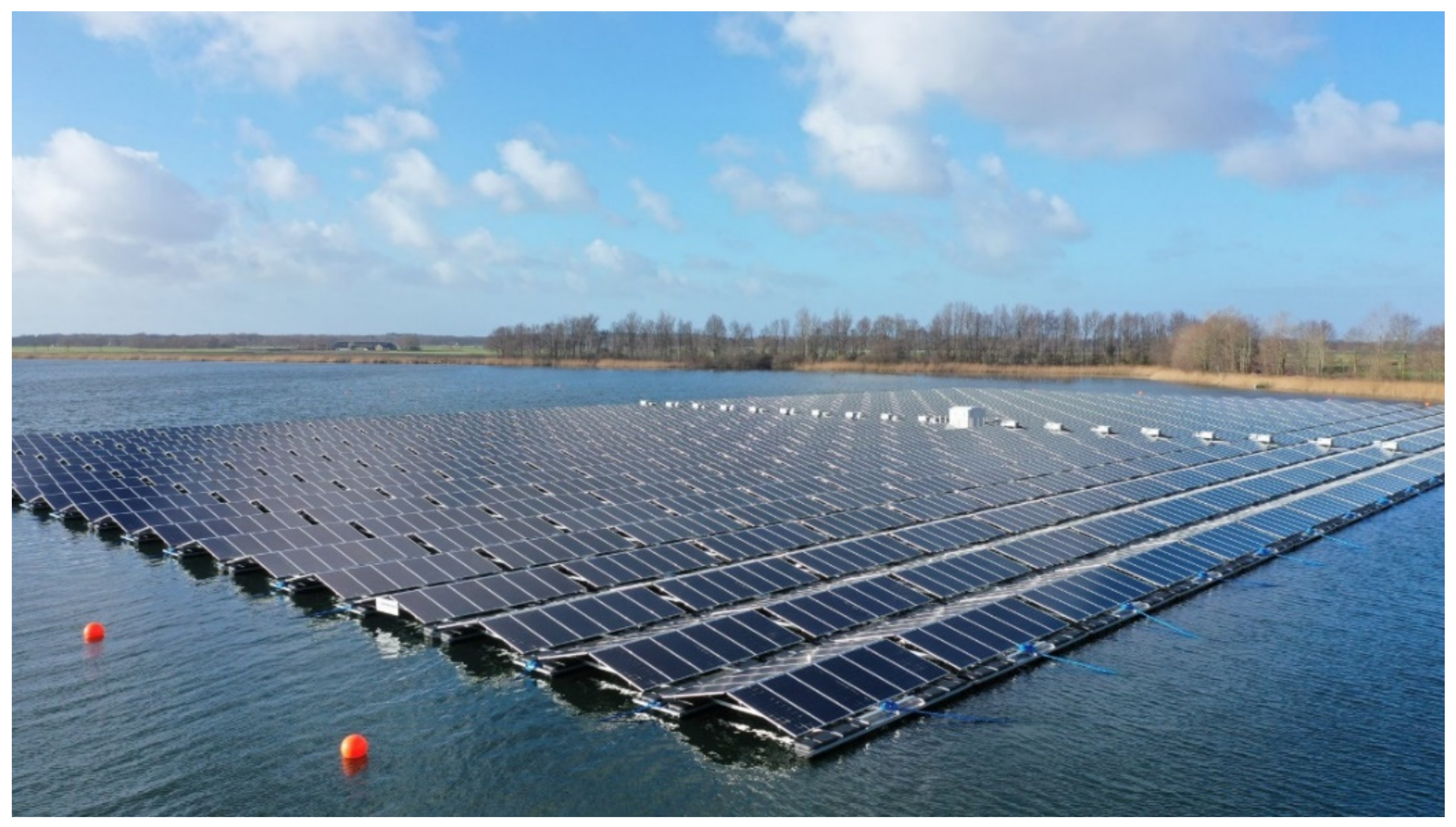
2.2. Groenleven Commercial Scale FPV System: Closed Structure

The commercial-scale FPV system by Groenleven is situated near the village of Oosterwolde in the Netherlands, on a sand extraction lake covering an area of approximately 23 hectares. This system consists of 5748 dual glass monocrystalline bifacial modules, each with a rated power of 365 Wp, resulting in a total installed power of 2.1 MWp. In Figure 2, a visual representation of the FPV system is presented. The modules are mounted in an East–West configuration, inclined at a tilt angle of 12°. The strings of modules are connected to a set of inverters (Huawei 36KTL), which are located on the FPV system itself. The FPV system is composed of interconnected “boats”, each housing 12 modules. To ensure buoyancy, HDPE floaters are used, encased by a metal structure to provide the necessary support. The measurement setup consists of several components. A Lufft WS600 UMB weather station is used to measure the ambient temperature, wind speed, and wind direction, providing comprehensive environmental data. Additionally, two class A EKO MS-80 pyranometers are used to record the POA irradiance. To monitor module temperature, PT100 sensors are installed on several representative locations (on the west side of the system). Water temperature is also measured using PT100 sensor. All gathered data are transmitted to a central measurement cabinet, which communicates with the central data server. The data are locally stored with a time resolution of 2 min and subsequently uploaded to the central server every 24 h. Within this study, measured data between April 2021 and March 2022 were recorded and used for analysis.

3. Analytical Methods

3.1. Datasets and Filtering

The measured data were aggregated to timesteps of 10 min. For the heat loss coefficient calculations, only data points during which the POA irradiance was greater than 250 W/m² were included. Furthermore, only the operational time of the PV systems was taken into consideration.

3.2. Wind Speed Height

The wind speed can fluctuate significantly depending on the elevation from the ground and the terrain’s roughness. In Oostvoorne, the wind speed was recorded at an approximate height of 3 m, whereas in Oosterwolde, it was measured at approximately 1.5 m above ground level. As a standard measurement height of 10 m is often used in meteorological databases, all recorded wind speeds were adjusted to correspond to a height of 10 m, using the following equation [19]:

$${\mathrm{V}}_{10}={\mathrm{V}}_{\mathrm{m}\mathrm{e}\mathrm{a}\mathrm{s}}\left(\frac{\mathrm{l}\mathrm{n}\left(\frac{10}{{\mathrm{z}}_0}\right)}{\mathrm{l}\mathrm{n}\left(\frac{{\mathrm{z}}_{\mathrm{m}\mathrm{e}\mathrm{a}\mathrm{s}}}{{\mathrm{z}}_0}\right)}\right)$$

(6)

The variable V₁₀ is the modeled wind speed at a height of 10 m (m/s), while V_meas represents the measured wind speed (m/s). The parameter z₀ refers to the roughness length of the surface (m), and z_meas indicates the height at which the wind speed is measured (m). The roughness length depends upon the type of surface and the landscape under investigation. The measurements were conducted in proximity to open water bodies. Thus, a standard roughness length value of 0.03 m was adopted, which is typically associated with grassland or open fields without obstacles.

3.3. Temperature Model including Water Temperature as a Variable

To investigate the impact of the surface water temperature on the PV module temperature, we used a regression correlation method. This method is founded on the steady-state energy balance approach, factoring in the water temperature. This steady-state heat transfer equation for FPV modules can be formulated as

$$G_{poa}\left(1-\eta \right)=U_c·\left(T_{mod}-T_{amb}\right)+U_v·v·\left(T_{mod}-T_{amb}\right)+U_w·(T_{mod}-T_{wat})$$

(7)

where G_poa is the incoming irradiance in W/m², $\eta$ is the module efficiency, U_c is the independent heat loss coefficient in W/m²K, v is the wind speed in m/s, U_v is the wind-dependent heat loss coefficient in W/m³Ks, and U_w is the surface water temperature-dependent heat loss coefficient in W/m²K.

As the module electric conversion efficiency η is temperature dependent, see Equation (1), this heat balance equation can be rewritten to calculate the modeled module temperature, as:

$$T_{mod}=\frac{T_{amb}\left(U_c+U_v·v\right)+U_w·T_{wat}+G_{poa}(1-{\eta }_{STC}\left(1-\gamma T_{STC}\right))}{U_c+U_{v}v+U_w+G_{poa}{\eta }_{STC}\gamma }$$

(8)

Temperature data exclusively from the commercial-scale Groenleven system were used to examine this model, considering surface water temperature as a variable.

4. Results and Discussion

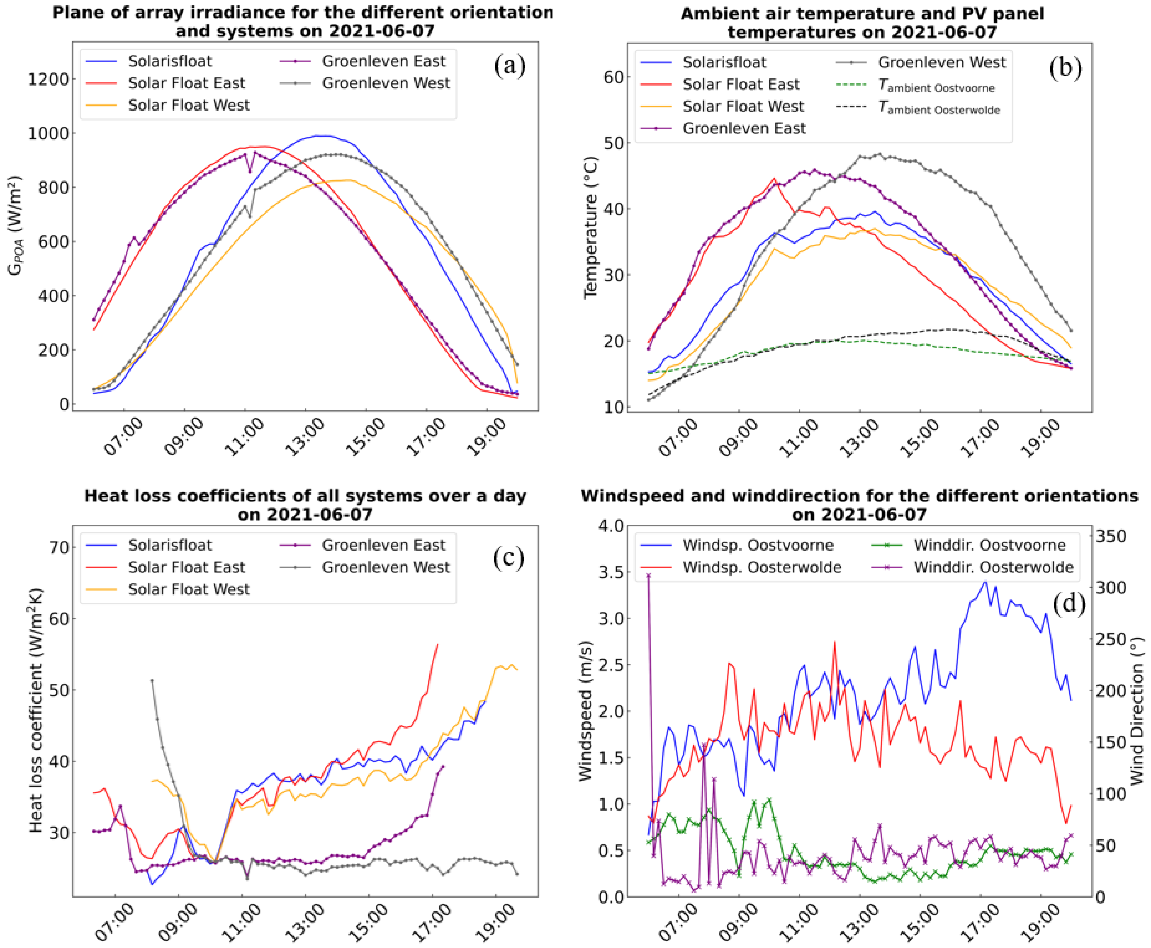
4.1. Thermal Behavior of the Different Systems on a Clear Sky Day

Figure 3 illustrates the thermal dynamics of the various FPV systems during a clear sky day at both different research sites. The different meteorological parameters, integral to calculating the heat loss coefficients, are also depicted in Figure 3a,b. In the periods just after sunrise and just before sunset, the operating temperature of PV modules not oriented towards the sun was observed to be lower than the ambient air temperature (Figure 3b). This discrepancy arises from the thermal radiation of the modules, a factor currently omitted from the heat loss coefficient equation, leading to an elevated heat loss coefficient during the periods when there is low irradiance, and the thermal radiation component is dominating the thermal behavior of the PV module.

On this specific day, the Solarisfloat system was orientated towards the West, and there was no sun tracking, as can be seen in the G_POA-irradiance data (Figure 3a), when the irradiance data from Solarisfloat and Solar Float west are compared. Examining the trend of heat loss coefficients (Figure 3c) throughout the day reveals that both the Solarisfloat and Solar Float systems exhibit coefficients roughly 10 W/m² to 15 W/m² higher than the Groenleven system between 10 a.m. and 4 p.m. Between 9 and 10 a.m., these coefficients are comparable. A notable shift in wind direction from East to Northeast at 10 a.m. in Oostvoorne (Figure 3d) enhances the wind exposure along the PV modules, likely contributing to more effective cooling. Between 10 a.m. and 12 p.m., meteorological conditions at Oostvoorne and Oosterwolde are highly similar, including the wind direction, wind speed, and ambient temperature. Despite comparable G_POA irradiance on the East modules of Groenleven and Solar Float, a lower measured panel temperature was observed in the Solar Float East modules at 10 a.m. This difference underscores a substantial reliance on the wind direction for the Solar Float system and to a lesser extent for the Groenleven system.

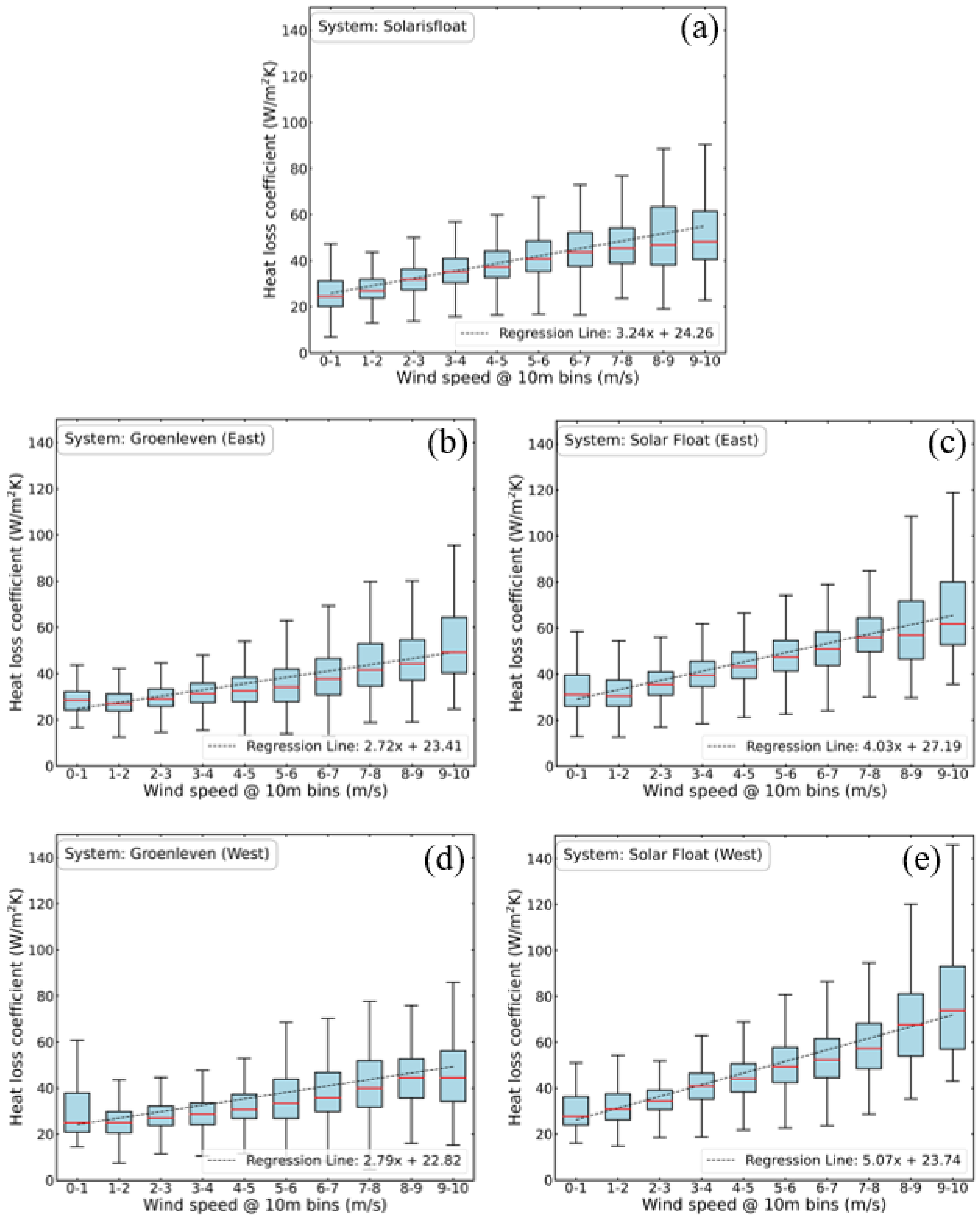
4.2. Heat Loss Coefficient

4.2.1. Wind Direction Independent

The boxplots displayed in Figure 4 show the heat loss coefficients categorized into various wind speed bins ranging from 0 to 10 m/s, each bin spanning a size of 1 m/s. Visualizing the influence of the wind speed on the heat loss coefficients. Additionally, a linear regression over the entire dataset is depicted, accompanied by the equation representing this linear regression. The results of the linear regression are also numerically displayed in

Table 2. Overview of the heat loss coefficients of the different PV systems as determined using linear regression.

System	Uc-Value [W/m2K]	Uv-Value [W/m3Ks]
Solarisfloat	24.3	3.2
Groenleven (East)	23.4	2.7
Solar Float (East)	27.2	4.0
Groenleven (West)	22.8	2.8
Solar Float (West)	23.7	5.1

, showcasing both the wind-independent U_c component and the wind-dependent U_v component for the various FPV systems and different panel orientations of the Groenleven and Solar Float system. Directing attention to the U_c component of these fittings reveals a relatively minor variation between different systems, ranging from 22.8 to 24.3 W/m²K, except for the Solar Float system with an East orientation, which records a value of 27.2 W/m²K. Distinctions among systems become more pronounced when considering the wind-dependent U_v heat loss coefficients. The Groenleven system demonstrates the lowest values in this respect, while the Solar Float exhibits the highest values. The U_v values of the Solarisfloat system are in between.

The observed discrepancy between the Solar Float and Groenleven systems is noteworthy as their panel orientation and system design is quite comparable. It suggests that the distinct sizing of these systems might play a significant role. Notably, the smaller Solar Float system appears to be more susceptible to the cooling effect of wind, resulting in a divergence in their respective wind-dependent heat loss coefficients. Furthermore, when comparing the Solarisfloat and Solar Float systems, the enclosed structure inherent in the Solar Float system design implies a potential challenge for wind to effectively cool the rear side of its modules. Despite this characteristic, the wind-dependent U_v value of the Solar Float system surpasses that of the Solarisfloat system.

4.2.2. Wind Direction Dependency

Figure 5 illustrates the wind roses for the two measurement sites, Oosterwolde and the Oostvoornse lake, during the measurement campaigns. Notably, the prevailing strong winds predominantly originate from the West, while there is a noticeable absence of wind from the Southwest direction. To explore the impact of wind direction on wind-dependent heat loss coefficients, an additional filtering mechanism based on wind direction (“North” encompassing Northwest to Northeast, “East” ranging from Northeast to Southeast, etc.) was applied to the datasets before conducting the linear regression fit. The wind-independent U_c value remained constant throughout the fit process, and the U_c value as determined in the original fit (as displayed in Section 4.2.1) was used.

The results of these fits can be seen in

Table 3. Wind direction-dependent U_v values of the different systems and panel orientations.

Wind Direction	Solarisfloat [W/m3Ks]	Groenleven (East) [W/m3Ks]	Solar Float (East) [W/m3Ks]	Groenleven (West) [W/m3Ks]	Solar Float (West) [W/m3Ks]
North	4.1	1.7	5.0	1.6	6.0
East	2.6	2.4	3.3	1.8	4.1
South	3.5	2.6	3.6	3.9	4.1
West	3.0	3.0	4.2	3.2	4.9

. Although the general trends as observed in the previous section are still present, it is noteworthy to point out that the wind-dependent heat loss coefficient of the Solar Float system is much higher (5.0 and 6.0 W/m³Ks) compared to the Groenleven system (1.6 and 1.7 W/m³Ks) during conditions when the wind has a directional component from the North. This advantage is likely facilitated by the system’s smaller scale, and the position of the measured modules (Northwest for the Solar Float system and West for the Groenleven system), allowing the wind to pass underneath more effectively, thereby facilitating the rear-side’s convective cooling. The outcomes of the Solarisfloat system are presented for completeness. However, it is challenging to draw any conclusions from these results, due to intermittent operational issues related to the system’s rotation, leading to an undefined orientation of the system with regard to the wind direction.

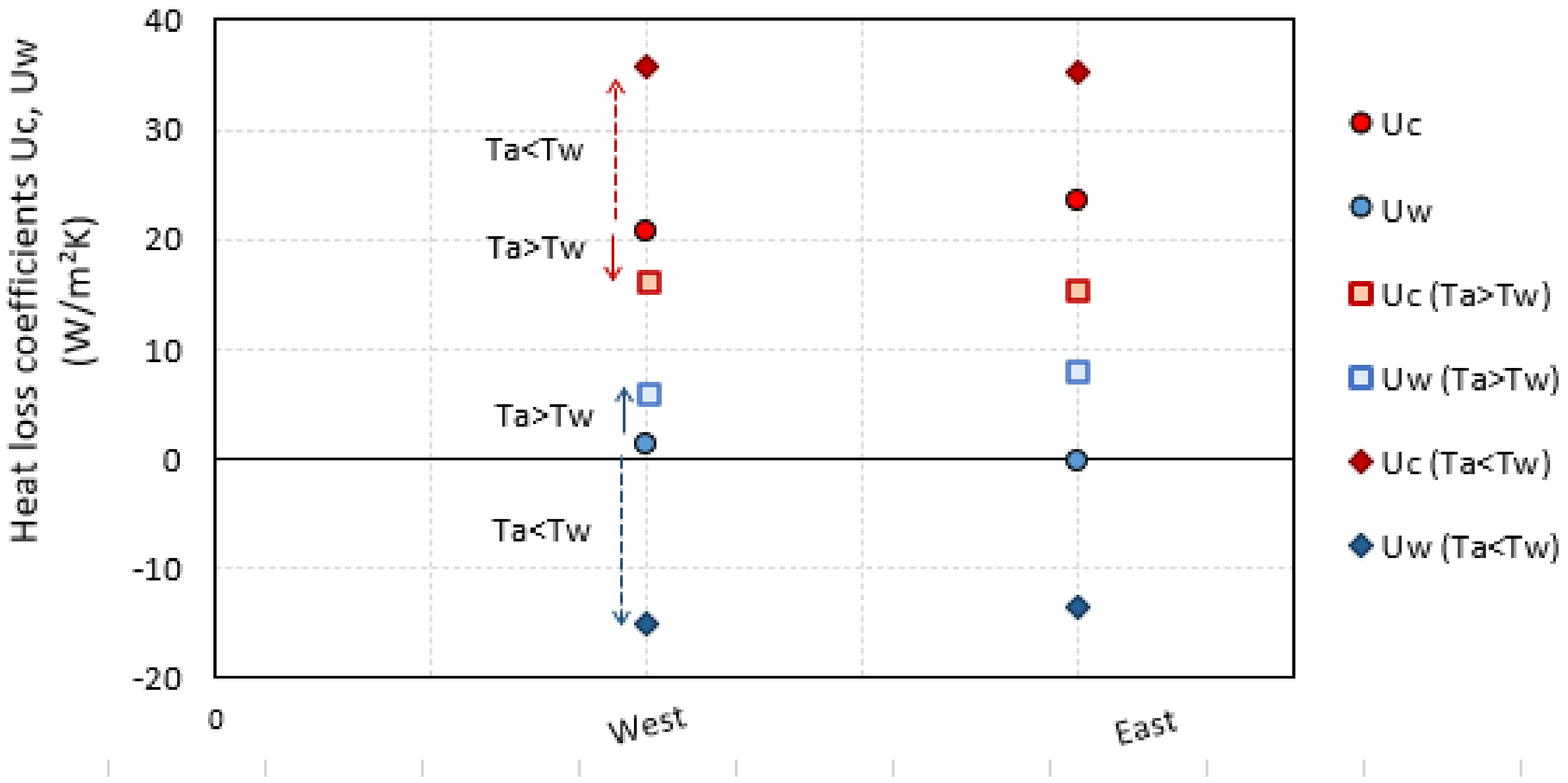
4.3. Thermal Model with Water Temperature

The Groenleven system served as the basis for the modeling, investigating the influence of the water temperature on the module temperature (Equation (8)). The analysis encompassed POA irradiances ranging from 100 to 1300 W/m², incorporating measured data from April 2021 to March 2022. Furthermore, it needs to be stated that the wind speeds as measured were used in this analysis, contrary to the previous section, where wind speeds were modeled to a height of 10 m. The resulting regression model provided the coefficients depicted in

Table 4. Results of the regression model for five modules, in terms of the different heat loss coefficients.

Orientation	Uc [W/m2K]	Uv [W/m3Ks]	Uw [W/m2K]
East	23.4	4.7	−0.3
West	20.6	5.1	1.4

.

The observed variability in the coefficient U_w, representing the heat loss coefficient dependent on surface water temperature, fluctuates between slightly positive and slightly negative values. This suggests a limited cooling impact, dependent on the surface temperature of the water, on the FPV modules, particularly within the context of this specific test site, and the ambient conditions. It is worth noting that, in this setup, the water is not directly in contact with the module surface. Additionally, an observation emerges: over the monitored period, the recorded water temperature hovered around the ambient temperature, with approximately equal durations of being higher and lower than the ambient temperature. This is shown in Figure 6, where the daily average temperature difference (weighted over irradiance) over the full measurement campaign is displayed (Figure 6a) together with the histogram (Figure 6b). This suggests both a heating and cooling effect due on the FPV module to the water surface temperature being both higher and lower compared to the ambient air temperature.

In the regression model, we focused solely on datapoints where T_amb > T_w would likely result in an increase in U_w accompanied by a proportional decrease in U_c. Conversely, we considered only datapoints where T_amb < T_w would lead to a significant decrease in U_w and a substantial increase in U_c, as depicted in Figure 7. However, conducting the model without accounting for U_w (thus excluding water temperature influence) would primarily cause a readjustment of the U_c coefficient. This adjustment ensures that the combined sum of both coefficients (U_c + U_w) remains approximately constant. This indicates that the heat loss coefficients U_c and U_w are strongly linked.

Scatter plots of measured and simulated module temperature values, using the model described in Equation (6), and the heat loss coefficients, as depicted in Table 4, are shown in Figure 8. The dashed black line acts as a guide for the eyes, where the modeled module temperatures are equal to the measured module temperatures. The color bar represents the wind speed. Overall, the scatter plots show that the model provides a good fit between the predicted and measured values. The R² value is around 0.96–0.97.

5. Concluding Remarks

This study contributes to the broader understanding of the thermal behavior of floating PV (FPV) systems by determining the heat loss coefficients of various systems. The Solar Float demonstrator system exhibits a notably higher heat loss coefficient, particularly evident in its considerably elevated wind-dependent heat loss coefficients of 4.0 and 5.1 W/m³Ks. In contrast, the Groenleven system, comparable in terms of system design, demonstrates lower wind-dependent heat loss coefficients of 2.7 and 2.8 W/m³Ks. Further investigation into this behavior reveals a disparity in wind-dependent heat loss coefficients, particularly pronounced with a North wind direction, indicating a more efficient convective cooling effect by the wind on the measured modules of the Solar Float demonstrator system. This could potentially be attributed to the wind’s enhanced ability to flow underneath the PV modules of the Solar Float system compared to the measured modules of the Groenleven system. The heat loss coefficients of the Solarisfloat system were moderately lower than those of the Solar Float system but higher than those of the Groenleven system. The results of this study indicate that in addition to considering the system’s design, the size of the FPV system also needs to be taken into consideration, when the wind-dependent heat loss coefficients are selected for determining the estimated annual yield.

The investigation into the influence of surface water temperature on the thermal behavior of the Groenleven FPV system involved incorporating a water temperature-dependent variable into an energy balance equation. Through linear regression, three heat loss coefficients were varied—U_c, U_v, and the water temperature-dependent U_w value. The findings suggest that while the water temperature can impact the PV panel temperature, the surface water temperature often exceeds the ambient air temperature, particularly during fall. This situation limits the water’s cooling effect on the FPV panel. In instances where the ambient air temperature is lower than the water temperature, the water’s presence results in the PV panel operating at a higher temperature. It is important to note the challenge of conducting multiple linear regressions with these three values. The interchangeability observed between the U_c and U_w values adds complexity to this analysis.

References

1. SolarPower Europe. Floating PV Best Practice Guidelines V1.0; SolarPower Europe: Brussels, Belgium, 2023; ISBN 978-9-464-66914-5. [Google Scholar]
2. Chowdhury, G.; Haggag, M.; Poortmans, J. How cool is floating PV? A state-of-the-art review of floating PV’s potential gain and computational fluid dynamics modeling to find its root cause. EPJ Photovolt. 2023, 14, 24. [Google Scholar] [CrossRef]
3. Woyte, A.; Richter, M.; Moser, D.; Reich, N.; Green, M.; Mau, S.; Beyer, H.G. Analytical Monitoring of Grid-Connected Photovoltaic Systems; IEA PVPS T13-03; IEA: Paris, France, 2014. [Google Scholar]
4. IEC61215-2; Terrestrial Photovoltaic (PV) Modules—Design Qualification and Type Approval—Part 2: Test Procedures. IEC: Geneva, Switzerland, 2021.
5. Skoplaki, E.; Palyvos, J.A. On the temperature dependence of photovoltaic module electrical performance: A review of efficiency/power correlations. Sol. Energy 2008, 83, 614–624. [Google Scholar] [CrossRef]
6. King, D.L.; Boyson, W.E.; Kratochvill, J.A. Photovoltaic Array Performance Model; Sandia National Laboratories (SNL): Albuquerque, NM, USA, 2004. [Google Scholar] [CrossRef]
7. Faiman, D. Assessing the outdoor operating temperature of photovoltaic modules. Prog. Photovolt. Res. Appl. 2008, 16, 307–315. [Google Scholar] [CrossRef]
8. Duffie, J.A.; Beckman, W.A. Solar Engineering of Thermal Processes, 4th ed.; Wiley: Hoboken, NJ, USA, 2014; pp. 757–759. ISBN 978-0-470-87366-3. [Google Scholar]
9. PVsyst: Array Thermal Losses. 1996. Available online: https://www.pvsyst.com/help/thermal_loss.htm (accessed on 21 February 2024).
10. Liu, H.; Krishna, V.; Lun Leung, J.; Reindl, T.; Zhao, L. Field experience and performance analysis of floating PV technologies in the tropics. Prog. Photovolta. Res. Appl. 2018, 26, 957–967. [Google Scholar] [CrossRef]
11. Dörenkämper, M.; Wahed, A.; Kumar, A.; De Jong, M.M.; Kroon, J.; Reindl, T. The cooling effect of floating PV in two different climate zones: A comparison of field test data from the Netherlands and Singapore. Sol. Energy 2021, 214, 229–247. [Google Scholar] [CrossRef]
12. Lindholm, D.; Kjeldstad, T.; Selj, J.; Marstein, E.S.; Fjær, H.G. Heat loss coefficients computed for floating PV modules. Prog. Photovolt. Res. Appl. 2021, 29, 1262–1273. [Google Scholar] [CrossRef]
13. Kjeldstad, T.; Lindholm, D.; Marstein, E.; Selj, J. Cooling of floating photovoltaics and the importance of water temperature. Sol. Energy 2021, 218, 544–551. [Google Scholar] [CrossRef]
14. Tina, G.M.; Bontempo Scavo, F.; Merlo, L.; Bizzarri, F. Comparative analysis of monofacial and bifacial photovoltaic modules for floating power plants. Appl. Energy 2021, 28, 116084. [Google Scholar] [CrossRef]
15. Dörenkämper, M.; de Jong, M.M.; Kroon, J.; Nysted, V.S.; Selj, J.; Kjeldstad, T. Modeled and Measured Operating Temperatures of Floating PV Modules: A Comparison. Energies 2023, 16, 7153. [Google Scholar] [CrossRef]
16. Fieldlab Westvoorne. Available online: https://www.fieldlabwestvoorne.nl/ (accessed on 21 February 2024).
17. TNO. Project Oostvoornse Meer; TNO: Delft, The Netherlands, 2022. [Google Scholar]
18. Groenleven. 2024. Available online: https://groenleven.nl/projecten/drijvend-zonnepark-oosterwolde/ (accessed on 21 March 2024).
19. Holton, J.R.; Hakim, G.J. Wind and Wind Systems. In Introduction to Dynamic Meteorology; Elsevier Academic Press: Amsterdam, The Netherlands, 2013; ISBN 9780123848666. [Google Scholar]
Figure 1. Pictures of both demonstrator-scale FPV systems, with the azimuthal tracking FPV system of Solarisfloat system on the left and the East–West facing FPV system of Solar Float on the right [17].
Energies 17 02027 g001
Figure 2. The commercial scale FPV system of Groenleven in Oosterwolde [18].
Energies 17 02027 g002
Figure 3. Ambient meteorological conditions and thermal behavior of the different systems on a single day. Indicated are the POA irradiances (a), ambient air and panel temperatures (b), wind speed and wind direction (c), and the calculated heat loss coefficients (d).
Energies 17 02027 g003
Figure 4. Boxplots with the heat loss coefficient as a function of the wind speed combined with the result of the linear regression of the different investigated PV systems ((a) Solarisfloat, (b) Groenleven (East), (c) Solar Float (East), (d) Groenleven (West), (e) Solar Float (West)).
Energies 17 02027 g004
Figure 5. Wind roses indicating the wind direction and wind speed (as a percentage of the total dataset) of the different sites: Oosterwolde (a) and Oostvoorne (b).
Energies 17 02027 g005
Figure 6. The ambient air temperature minus the surface water temperature (weighted over irradiance) during the full measurement campaign (a) and a histogram showing these temperature differences (b).
Energies 17 02027 g006
Figure 7. Variation of coefficients Uc and Uw at varying datasets (no filter, Tamb > Tw, Tamb < Tw).
Energies 17 02027 g007
Figure 8. Scatter plots showing the comparison between the measured and simulated Tmodule for all the considered modules, as a function of the wind speed (color bar).
Energies 17 02027 g008