Optimizing the Building Refurbishment Process Using Improved Evolutionary Algorithms

Abstract

An optimization model that may be applied to analyze building retrofit strategies is presented in this research. The aim of this research paper is to identify the optimal thermal envelope configuration that will assure the minimum energy requirement for heating in the case of a residential building, while also considering price restrictions obtained through a specific market survey. To achieve this, several values for the following parameters are considered: thermal insulation materials’ conductivities and thicknesses, windows’ overall heat transfer coefficients and total solar energy transmittance and doors’ thermal proprieties. Additionally, this paper presents a method used to find the best option from among the available heat pumps that could cover most of the energy requirements for heating and domestic hot water systems, also considering the products’ prices. The proposed method is based on a Non-dominated Sorting Genetic Algorithm II (NSGA-II) model developed in the Pymoo (Multi-Objective Optimization in Python) library. The result shows that the energy requirement for heating can be reduced by up to approximately 75% compared to that obtained in the case of a non-insulated building by using suitable insulation materials and doors and windows with superior thermal proprieties chosen by the NSGA-II.

1. Introduction

Buildings, as significant energy consumers that are steadily growing, are a crucial actor in the European Union’s (EU’s) energy plan. Buildings account for over 40% of the total energy consumed in the EU sectors [1]. Approximately 45% of the total primary energy consumption in Romania is attributed to the country’s building stock, which mainly consists of old and energy-inefficient buildings [2]. Approximately 75% of all building structures in the EU are residential, and the large majority (80%) were built before 1991, when no energy-efficiency guidelines were available, suggesting inadequate or nonexistent thermal insulation [3]. These facts highlight the necessity of appropriate and prompt action aimed at mitigating the energy impact of buildings across the EU. For these reasons, new methods for improving the energy efficiency of existing buildings are continuously studied.

A comprehensive literature survey showed that different optimization methods have been successfully applied for analyzing buildings’ energy infrastructure, but few publications have taken price constraints into consideration. For example, in ref. [4], a comprehensive study regarding combining EnergyPlus V8.4.0 (building energy simulation tool) simulation results with the NSGA-II was presented, thus obtaining the optimal solutions to improve the building’s energy performance. Additionally, the effects of the building orientation, window sizes and the overhang specifications on the annual cooling and lighting building energy demands were studied in Iran’s four climate zones. The objective functions were minimizing the annual cooling and lighting energy consumptions. The results showed that the optimum configuration reduced the total annual building energy consumption by up to 23.8%.

The refurbishment process optimization was analyzed in a region of Finland, where a building constructed in 1960s was considered [5]. Here, an NSGA-II was developed to identify the best refurbishment strategies for the energy performance of the building, while also considering the minimization of the implicit life-cycle costs. The following renovation solutions were analyzed: the thermal insulation of the external walls, the use of PV production systems and several heat pump systems. The results underlined that the ground source heat pump has the greatest economic feasibility and causes the biggest improvement in the energy performance of the building.

A Non-dominated Sorting Genetic Algorithm II was also developed in the case of a residential building located in the Bahamas to optimize the carbon emissions and life-cycle costs [6]. The variables used in this algorithm were the type of thermal insulation used for the walls and the type of roof construction (standard, insulated, reflective and reflective–insulated), both the type of window glazing and the lighting systems, the surface, the tilt, and azimuth angles of the photovoltaic panels, and finally, the storage battery capacity. The results showed that the optimal solutions are obtained when using insulation with thermal resistance between 6 and 7 (m²·K)/W for the interior walls and between 6 and 10 (m²·K)/W for the roof, and double-glazed windows with a low emissivity coating.

A comprehensive thermal envelope optimization strategy was analyzed for a residential building located in Turkey, also using the NSGA-II developed in MATLAB [7]. The objective functions were minimizing the energy required for heating and cooling under investment cost constraints. The optimization algorithm was developed considering the fallowing variables: the building’s orientation, thermal envelope’s material types and thickness, and windows’ type and dimensions. The results underlined that non-dominated solutions were in the range of $135,000 to $205,000 in terms of the initial investment cost in the case of this heating climate zone. The optimal energy required for heating and cooling varied between 211,000 and 272,000 kWh.

A similar approach was considered for a building located in France [8]. Here, the objective functions were minimizing the building’s primary energy consumption for heating and lighting and the degree–hours of summer thermal discomfort. The results showed that the optimal solution for the northern regions of France was obtained when using a well-insulated envelope, small skylight area, and standard roof. In the case of the southern region, the optimal solutions had a non-insulated ground slab, reflective cool roof, and large skylight area. The optimal building energy consumption varied between 18.9 kWh/m²/year in case of the southeastern area and 65.7 kWh/m²/year in case of the northeastern area.

An NSGA-II algorithm written in the Java programming language was used to optimize the heating and cooling energy consumption in the study from ref. [9]. The variables used in this algorithm were the windows’ properties and configuration and the rooms’ position, floor height and wall orientation. The selection of an appropriate window size and orientation was made considering the facts that it must assure proper daylighting and natural ventilation and decrease or increase the solar radiation gained, depending on the season. The optimal configuration was a window positioned at the center (1.1 m away from the edge) having around a 48% window-to-wall ratio (WWR) with a horizontal configuration. By using this configuration, a reduction of 26.1% in the annual energy consumption was obtained in the case of a room located on the 15th floor compared to the baseline room model.

The GBDT (Gradient-Boosting Decision Tree) and NSGA-II algorithms were combined to optimize the energy consumption and thermal comfort of residential buildings in China [10]. Twenty passive design parameters were analyzed, including the effects of windows on natural ventilation. According to the optimization results, there was an 88.2% energy savings rate and a 37.8% improvement in thermal comfort compared to the base-case construction.

A Non-dominated Sorting Genetic Algorithm-II was combined with a Multilayer Perception Artificial Neural Network (MLPANN) metamodel to maximize the energy efficiency and thermal comfort of a building in China [11]. The results pointed out that, by using the optimal building design, the heating energy consumption could be reduced by up to 78.2% and the cooling energy consumption decreased by 71.3% compared to the initial configuration.

A recent study presented in ref. [12] combines a Bayesian optimization with extreme gradient-boosting trees (BO-XGBoosts) with an NSGA-II to optimize a residential building’s performances. The objective functions were minimizing the building’s energy consumption and maximizing the daylighting performance and indoor thermal comfort. The results showed that by using the optimal configuration, the energy consumption was decreased by 44.1%, thermal comfort index was reduced by 10.9%, and daylighting performance was improved by 1.7% compared to the initial configuration.

Starting from this literature survey, the present paper proposes a method for determining the optimal thermal envelope configuration in the case of a generic building located in Bucharest, Romania, considering two requirements: obtaining the minimum energy requirement for heating and also considering the price restrictions obtained through a specific market survey. The current research is an improved version of the optimization method studied in the article entitled “Optimization of energy rehabilitation processes of existing buildings”, authors: A.E. Nicolae, H. Necula, and B. Căruțașiu, in which a simplified model to optimize the energy required for heating and the cost of the insulation materials was presented [13]. The differences between the simplified model and the improved variant are the following:

• In the simplified model, a Genetic Algorithm (GA) was used, while the current approach proposes a Non-dominated Sorting Genetic Algorithm (NSGA-II).
• The simplified model did not use the Pymoo (Multi-Objective Optimization in Python) library.
• The simplified model had fewer variables and input data than the improved model; thus, the windows’ overall heat transfer coefficients and total solar energy transmittance and the doors’ thermal proprieties were not initially simulated and predetermined thermal proprieties were used. The search space was represented by only thickness–thermal conductivity pairs. In addition, the exterior walls and the floor were insulated with expanded polystyrene and extruded polystyrene, but the roof-ceiling was not insulated.
• In the simplified model, the computational outdoor temperature was considered −15 °C, according to the SR1907-1 Standard [14]. The average value of the solar radiation intensity was considered to be 77.03 W/m² [15]. The current model uses the monthly average solar radiation intensity and the monthly average outdoor temperature.
• In the simplified model, the average ground temperature was considered to be θ_ground = 10 °C at a depth of 2 m (δ_p) according to [16].
• The simplified model did not include the heat pump-choosing algorithm.

The current research is structured as follows. Section 2 presents the steps taken in developing an NSGA-II (Non-dominated Sorting Genetic Algorithm II). Section 3 places an emphasis on the application of a Non-dominated Sorting Genetic Algorithm II in the case of the studied building, with the exterior walls insulated with expanded polystyrene, the floor insulated with extruded polystyrene and the roof–ceiling insulated with mineral wool. The NSGA-II model was developed in the Pymoo (Multi-Objective Optimization in Python) library. It was used to find the optimal choice among a considered search space comprising different values of thicknesses and thermal conductivities for insulation materials, and thermal properties for both windows and doors. The model indicates the materials that ensure the lowest energy requirement for heating, while also considering price restrictions obtained through a specific market survey. Finally, Section 4 presents a method, implemented in Python V3.11, to find the best heat pumps that cover most of the energy requirements for heating and domestic hot water systems, considering two important variables: the energy performances and the unit price.

2. The Steps of the Non-Dominated Sorting Genetic Algorithm II

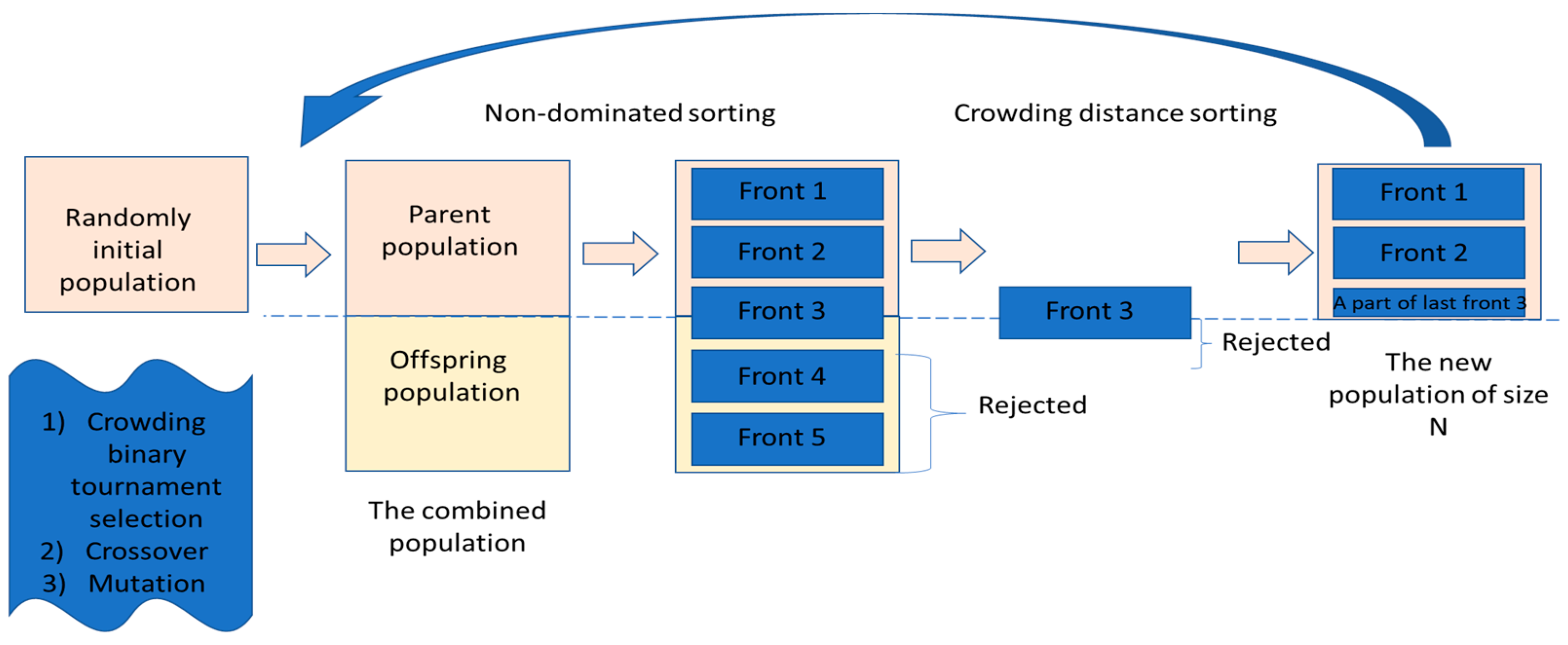
The Non-dominated Sorting Genetic Algorithm II was developed by Deb et al. in 2002 [17]. The algorithm is very similar to the GA. The NSGA-II differs from the simple GA in the way of selecting the parents, because the NSGA-II uses non-dominated sorting and crowding-distance sorting. The NSGA-II model’s development requires implementing the following procedures:

• Establishing the input parameters: the population size, the number of generations, crossover probability, and mutation probability [18]. A random initial population is generated. The objective functions are evaluated. The parents are selected using crowding binary tournament selection.
• Creating the offsprings from the initial parents using the standard operators of the GA (crossover and mutation); thus, a combined population consisting of parents and offspring is created [19].
• Sorting the combined population based on the non-dominated ranks and crowding-distance. Several non-dominated fronts (Pareto fronts) are produced. Each member in each front has assigned a fitness value or rank [20].

“Pareto Front is a set of nondominated solutions, being chosen as optimal, if no objective can be improved without sacrificing at least one other objective” [21]. The dominance principle is as follows: “A solution x is said to dominate the other solution y if the solution x is no worse than y in all objectives and the solution x is strictly better than y in at least one objective” [18].

If the size of the first front is less than N, where N represents the size of the population, all the individuals from this front will be chosen for the new generation. The remaining individuals, calculated as a difference between the size N of the population and the number of individuals belonging to the first non-dominant front, are chosen from the next non-dominated fronts in the order of their rank, maintaining the same rule. Some of the individuals from the last front are selected to pass into the next generation using the crowding-distance comparison operator in descending order [17]. In other words, only some of the individuals belonging to the first dominant front pass into the next generation. The best N individuals with higher diversity are selected using the non-dominated sorting and crowding-distance sorting, while discarding the rest of the solutions [22]. The whole of this complex process is summarized in Figure 1.

Elitism is also used to ensure that the individuals belonging to the higher-ranking fronts are kept and passed to the next generation. According to the elitism paradigm, the best individuals from the previous generation are copied into the next generation without any changes. In this way, the convergence speed of the algorithm increases [23]. In crowding-distance sorting, individuals are ranked inside a front based on how far apart their two closest neighbors are from one another. It is preferable that the crowding distance has a large value [24].

4.

Application of crossover and mutation to the new population of size N to produce a new combined population consisting of parents and offspring. The algorithm keeps running from step 2 until the maximum number of generations is achieved [25].

3. Case Study

In this study, a hypothetical facility located in Bucharest, Romania, emulating a single-family residential building, was proposed. The monthly average solar radiation intensity for the Bucharest area was considered according to Methodology MC001—Part I, annex A.9.6, the monthly average of the outdoor temperatures according to SR4839 Standard, while the ground temperature was obtained from the RETScreen software V9.0 [26,27]. These data are summarized in

Table 1. Climate data from the Bucharest area.

Month	The Monthly Average Solar Radiation Intensity [W/m2]	The Monthly Average Outdoor Temperature [°C]	Ground Temperature [°C]
January	59.3	−1.4	−2.2
February	87.3	0.1	0.0
March	91.4	5.1	5.5
April	91.6	11.1	12.0
May	86.0	16.8	18.3
June	92.8	20.7	23.1
July	89.9	22.6	26.0
August	123.8	21.8	25.6
September	119.1	16.5	19.5
October	104.1	10.5	12.2
November	57.4	4.5	5.2
December	53.0	−0.3	−0.7

.

According to the national SR1907-2 standard [28], the computational indoor temperature was considered to be 20 °C for the heating period. The aim of this study was not to analyze the thermal coupling of the interior thermal zones between different rooms. Thus, the building was considered a single thermal zone, having a constant interior temperature of 20 °C. Moreover, it was considered that the heating season lasts 4536 h per year: 744 h in January, March, October and December, 720 h in November, 672 h in February and 168 h in April. Based on the SR 4839 standard, the heating season in the Bucharest area lasts 189 days, assuming an average outdoor temperature of 12 °C and a computational indoor temperature of 20 °C [27].

In the case of the non-insulated building, it was considered that the windows have an overall heat transfer coefficient (U_w—value) of 5.4 W/(m²·K) and total solar energy transmittance of 0.85. The door has an overall heat transfer coefficient of 2.47 W/(m²·K). The U values of the exterior walls, of the floor and of the roof–ceiling before the thermal insulation of the envelope were 0.723 W/(m²·K), 0.485 W/(m²·K) and 2.718 W/(m²·K). These values were obtained considering the heat transfer by conduction and convection and the thermal resistance of the ground. The energy requirement for heating in the case of the non-insulated building was 385.128 kWh/m²/year (this value was obtained before applying the thermal renovation measures). This value took into consideration the heat losses by infiltration and the heat transfer by transmission between the heated space and the outside environment due to temperature differences but did not consider the thermal mass, thermal inputs from solar radiation and internal heat gains from occupants, equipment, and lighting.

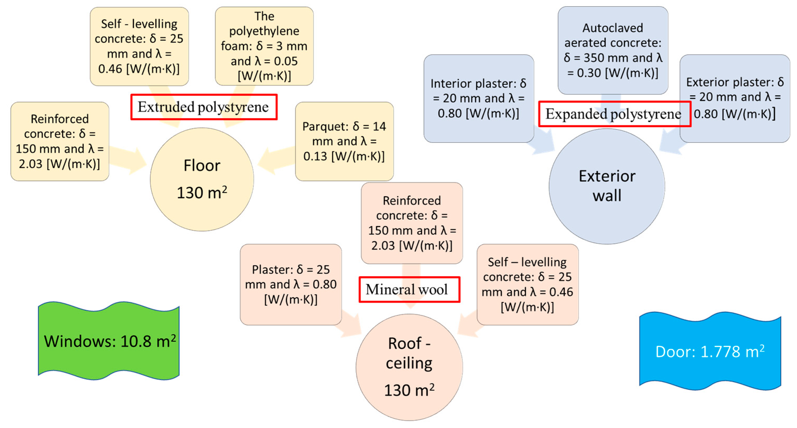
To reduce this value, the exterior walls, floor, and roof–ceiling were insulated with expanded polystyrene, extruded polystyrene and mineral wool, respectively. The door and the windows were replaced with ones with superior thermal proprieties, as presented in Section 3.3. Figure 2 specifies the construction materials in the case of the non-insulated and insulated buildings (the insulation materials are written in the red boxes).

Furthermore, a Non-dominated Sorting Genetic Algorithm II is developed in Pymoo, aiming to identify the optimal choice among the various values of thicknesses and thermal conductivities for the insulation materials, and the thermal properties for both the windows and doors, considering two requirements: obtaining the lowest energy requirement for heating and also considering the price restrictions obtained through a specific market survey.

3.1. Optimization Problem Development

The first step in the simulation was to define the problem optimization inherited from the ElementwiseProblem (object-oriented definition, which implements a function evaluating a single solution at a time) object. The problem’s properties, such as the number of variables (n_var), objectives (n_obj) and constraints (n_constr), were set [29]. An objective function was defined (minimizing the function of energy requirement for heating) with five price inequality constraints, so n_obj = 1 and n_constr = 5. The aim was to find the best solutions that satisfy all the constraints associated with the objective function [30]. The variables (n_var = 9) used in the simulation were the following:

• Thermal conductivities and thicknesses of expanded polystyrene, extruded polystyrene and mineral wool in case of the walls, floor and roof–ceiling.
• Overall heat transfer coefficient and total solar energy transmittance for the windows.
• Overall heat transfer coefficient in case of the door.

A function named _evaluate was implemented to evaluate the objective function. The output of this customed function is written to the dictionary output with the key F as a NumPy array object [29]. G is the key for the constraints. The optimization problem to be implemented is given by:

$$\begin{gathered} \mathit{min}{Q}_{heating}\left({\delta }_{ins1},{\lambda }_{ins1, }{\delta }_{ins2},{\lambda }_{ins2, }{\delta }_{ins3},{\lambda }_{ins3, }{U}_w,g, U_2\right) \\ ={\sum }_k{h}_k·\left[\begin{array}{c}{\Delta T}_k·H_V+q_{1k}\left({\delta }_{ins1},{\lambda }_{ins1}\right)·\left(A_1{+A}_2+A_3+A_4\right)+q_{2k}\left({\lambda }_{ins2, }{\delta }_{ins2}\right)\\ ·A_5+q_{3k}\left({\lambda }_{ins3, }{\delta }_{ins3}\right)·A_6+q_{4k}\left(g,U_w\right)·A_7+q_{5k}\left(U_2\right)·A_8\end{array}\right] \left[\frac{\mathrm{k}\mathrm{W}\mathrm{h}}{\mathrm{y}\mathrm{e}\mathrm{a}\mathrm{r}}\right] \end{gathered}$$

(1)

k = January, February, March, April, October, November, December.

In Pymoo, it is necessary to formulate the inequality constraints as less than zero. This will be applied when dealing with price constraints. Consequently, a survey was conducted and several price combinations for each configuration (consisting of different pairs of thermal properties) were obtained from manufacturers’/retailers’ websites. Hence, P_i (δ_{ins i}, λ_{ins i}) represents the prices of insulation materials for different combinations of thicknesses (δ_{ins i}) and thermal conductivities (λ_{ins i}). Similarly, P₄ (g, U_w) represents the prices of windows, while P₅ (U₂) contains the prices of different types of doors. These values were further used to compute the mean values of the prices for each configuration (consisting of different pairs of thermal properties), resulting the following values: 42.41 RON/m²—for expanded polystyrene, 78.91 RON/m²—for extruded polystyrene and 91.09 RON/m²—for mineral wool. In the case of the windows and doors, these prices were set at 1500 RON/piece and 6574.63 RON/piece. The current exchange rate of Euro (€) to Romanian leu (RON) is EUR 1 = RON 4.97. Consequently, the five price constraints are defined as follows:

$$P_1\left({\delta }_{ins1},{\lambda }_{ins1}\right)-42.41 \le 0 [\mathrm{R}\mathrm{O}\mathrm{N}/{\mathrm{m}}^2]$$

(2)

$$P_2\left({\delta }_{ins2},{\lambda }_{ins2}\right)-78.91 \le 0 [\mathrm{R}\mathrm{O}\mathrm{N}/{\mathrm{m}}^2]$$

(3)

$$P_3\left({\delta }_{ins3},{\lambda }_{ins3}\right)-91.09 \le 0 [\mathrm{R}\mathrm{O}\mathrm{N}/{\mathrm{m}}^2]$$

(4)

$$P_4\left(g, U_w\right)-1500 \le 0 \left[\mathrm{R}\mathrm{O}\mathrm{N}\right]$$

(5)

$$P_5\left(U_2\right)-6574.63 \le 0 \left[\mathrm{R}\mathrm{O}\mathrm{N}\right]$$

(6)

The lower (x_l) and upper (x_u) variable boundaries are:

$$20\le {\delta }_{ins1} \le 150 \left[\mathrm{m}\mathrm{m}\right]$$

(7)

$$0.036 {\le \lambda }_{ins1} \le 0.042 [\mathrm{W}/(\mathrm{m}·\mathrm{K}\left)\right]$$

(8)

$$10\le {\delta }_{ins2} \le 100 \left[\mathrm{m}\mathrm{m}\right]$$

(9)

$$0.031\le {\lambda }_{ins2} \le 0.039 [\mathrm{W}/(\mathrm{m}·\mathrm{K}\left)\right]$$

(10)

$$30\le {\delta }_{ins3} \le 200 \left[\mathrm{m}\mathrm{m}\right]$$

(11)

$$0.034\le {\lambda }_{ins3} \le 0.038 [\mathrm{W}/(\mathrm{m}·\mathrm{K}\left)\right]$$

(12)

$$0.4\le g\le 0.85 \text{[-]}$$

(13)

$$0.6\le U_w \le 5.4 [\mathrm{W}/({\mathrm{m}}^2·\mathrm{K}\left)\right]$$

(14)

$$0.7\le U_2 \le 2.47 [\mathrm{W}/({\mathrm{m}}^2·\mathrm{K}\left)\right]$$

(15)

where Q_heating = the energy requirement for heating [kWh/year]; h_k = the heating period [hours]; H_V = the heat loss coefficient of the building through ventilation [W/K]; ΔT_k = the temperature difference [°C]; δ_ins1, δ_ins2, δ_ins3 = the thickness of the expanded polystyrene, extruded polystyrene and mineral wool [mm]; λ_ins1, λ_ins2, λ_ins3 = the thermal conductivities of the expanded polystyrene, extruded polystyrene and mineral wool [W/(m·K)]; U_w, U₂ = the overall heat transfer coefficients of windows and doors [W/(m²·K)]; g = the total solar energy transmittance [-]; A₁, A₂, A₃, A₄, A₅, A₆, A₇, A₈ = the areas of the construction elements (western, eastern and northern walls, unglazed surface of the southern wall, floor, roof–ceiling, door and windows [m²]; q_1k (δ_ins1, λ_insl1), q_2k (δ_ins2, λ_ins2), q_3k (δ_ins3, λ_ins3), q_4k (g, U_w), q_5k (U₂) = the heat fluxes through the walls, floor, roof–ceiling, windows and door [W/m²].

The linear dimensions of the studied single-floor building are presented in Figure 3. The areas of the construction elements are: A₁ = A₂ = 15.6 m²; A₃ = 48.0 m²; A₄ = 35.4 m²; A₅ = A₆ = 130.0 m²; A₇ = 10.8 m²; A₈ = 1.8 m².

The heat loss through ventilation coefficient of the building, H_V, is determined using the relation (16):

$$H_V=\frac{{\rho }_a{c}_a{n}_{a}V}{3.6} \left[\frac{\mathrm{W}}{\mathrm{K}}\right]$$

(16)

where ρ_a = the air density; c_a = the specific heat of air; n_a = the average number of air changes; V = heated volume. These parameters are considered: ${\rho }_a=1.2 \frac{\mathrm{k}\mathrm{g}}{{\mathrm{m}}^3}$; $V=312 {\mathrm{m}}^3;c_a=1.005 \frac{\mathrm{k}\mathrm{J}}{\mathrm{k}\mathrm{g}\mathrm{K}}$; $n_a=0.6 {\mathrm{h}}^{-1}$ [31].

In the case of the heat fluxes, the Fourier unidirectional conduction equation is written for each of the building’s components: walls (relation 17), floor (relation 18) and roof–ceiling (relation 19). The heat fluxes q_4k (g, U_w) and q_5k (U₂) for the windows and door are computed using relations (20) and (21).

$$q_{1k}\left({\delta }_{ins1}, {\lambda }_{ins1}\right)=\frac{{\theta }_{in}-{\theta }_{ out k}}{\frac{1}{{\alpha }_{1in}}+\frac{{\delta }_1}{{\lambda }_1}+\frac{{\delta }_2}{{\lambda }_2}+\frac{{\delta }_3}{{\lambda }_3}+\frac{{\delta }_{ins1}}{{\lambda }_{ins1}}+\frac{1}{{\alpha }_{1out}}}\left[\frac{\mathrm{W}}{{\mathrm{m}}^2}\right]$$

(17)

$$q_{2k}\left({\delta }_{ins2}, {\lambda }_{ins2}\right)=\frac{{\theta }_{in}-{\theta }_{ground k}}{\frac{1}{{\alpha }_2}+\frac{{\delta }_1}{{\lambda }_1}+\frac{{\delta }_2}{{\lambda }_2}+\frac{{\delta }_3}{{\lambda }_3}+\frac{{\delta }_4}{{\lambda }_4}+\frac{{\delta }_{ins2}}{{\lambda }_{ins2}}+\frac{{\delta }_{1p}}{{\lambda }_{1p}}+\frac{{\delta }_{2p}}{{\lambda }_{2p}}}\left[\frac{\mathrm{W}}{{\mathrm{m}}^2}\right]$$

(18)

$$q_{3k}\left({\delta }_{ins3}, {\lambda }_{ins3}\right)=\frac{{\theta }_{in}-{\theta }_{ out k}}{\frac{1}{{\alpha }_{3in}}+\frac{{\delta }_1}{{\lambda }_1}+\frac{{\delta }_2}{{\lambda }_2}+\frac{{\delta }_3}{{\lambda }_3}+\frac{{\delta }_{ins3}}{{\lambda }_{ins3}}+\frac{1}{{\alpha }_{3out}}}\left[\frac{\mathrm{W}}{{\mathrm{m}}^2}\right]$$

(19)

$$q_{4k}\left(g,U_w\right)=U_w·\left({\theta }_{in}-{\theta }_{ out k}\right)+G_k·\mathrm{g}\left[\frac{\mathrm{W}}{{\mathrm{m}}^2}\right]$$

(20)

$$q_{5k}\left(U_2\right)=U_2·\left({\theta }_{in}-{\theta }_{ out k}\right)\left[\frac{\mathrm{W}}{{\mathrm{m}}^2}\right]$$

(21)

where θ_in = computational indoor temperature [°C]; θ_{out k} = monthly average outdoor temperature presented in Table 1 [°C]; θ_{ground k} = ground temperature presented in Table 1 [°C]; α_1in, α_1out, α₂, α_3in, α_3out = convection heat transfer coefficient [W/(m²·K)]; δ₁, δ₂, δ₃, δ₄ = thickness of the construction materials in case of exterior walls, floor or roof–ceiling shown in Figure 2 [mm]; λ₁, λ₂, λ₃, λ₄ = thermal conductivities of the construction materials in the case of exterior walls, floor or roof–ceiling shown in Figure 2 [W/(m·K)]; δ_ins1, δ_ins2, δ_ins3 = thickness of the expanded polystyrene, extruded polystyrene and mineral wool [mm]; λ_ins1, λ_ins2, λ_ins3 = thermal conductivities of the expanded polystyrene, extruded polystyrene and mineral wool [W/(m·K)]; δ_1p, δ_2p = depth in the ground [mm]; λ_1p, λ_2p = ground thermal conductivity [W/(m·K)]; U_w, U₂ = the overall heat transfer coefficients [W/(m²·K)]; g = total solar energy transmittance [-]; G_k = monthly average solar radiation intensity presented in Table 1 [W/m²].

For computing q_1k (δ_ins1, λ_ins1), the convection heat transfer coefficients are considered: α_1in = 8 W/(m²·K) and α_1out = 24 W/(m²·K) [15]. According to [16], the convection heat transfer coefficient used to calculate the thermal resistances of construction elements in contact with the ground is: α₂ = 6 W/(m²·K). At the depth of 1.2 m (δ_1p), thermal conductivity has the value λ_1p = 2 W/(m·K), and at the depth of 4 m (δ_2p), it is considered λ_2p = 4 W/(m·K) [16]. To compute q_3k (δ_ins3, λ_ins3), the convection heat transfer coefficients are considered: α_3in = 8 W/(m²·K) and α_3out = 12 W/(m²·K) [15].

Several types of glazing are considered, such as clear float glass; double-glazed insulating glass units (IGUs) consisting of two float glasses separated by a compact layer of air; double-glazed IGUs with one float glass and one low emissivity (low—E) glass separated by air or argon; four seasons (4S) double-glazed IGUs consisting of a float glass and a 4S glass separated by argon; triple-glazed IGUs with three float glasses separated by a compact layer of air; triple-glazed IGUs with two 4S glasses and one float glass, separated by argon; triple-glazed IGUs with one float glass and two low—E glass, separated by argon or krypton; triple-glazed IGUs with two float glasses and one low—E glass, separated by argon; triple-glazed IGUs with one 4S glass, one float glass and one low—E glass, separated by argon; triple-glazed IGUs with one 4S glass and two float glasses separated by argon or air. Moreover, we considered wood, glass, metal, medium-density fiberboard (MDF), polyvinyl chloride (PVC) and plasticized polyvinyl chloride (UPVC) doors.

3.2. Initialize the NSGA-II

Sampling was used to create the initial population. The function np.random.random_sample() was implemented for performing random sampling in numpy. The population size was set at 40 individuals. The studied NSGA-II only generates 10 offspring in each generation. A Steady State Selection was used. Two parents were randomly selected to produce children, and then the children resulting from the processes of crossover and mutation were introduced into the population [32]. The size of the population must remain constant, so a sorting of individuals according to their fitness was carried out. If the children are more adapted than the two weakest individuals in the population, then they replace them so that the population remains constant [33].

Additionally, a duplicate check was implemented to verify if the algorithm produces offspring that differ from the current population in terms of their variable vectors as well as from themselves [29]. The NSGA-II was set to stop after considering 200 generations.

In the case of crossover, we used the Simulated Binary Crossover (SBX) with the probability distribution equal to 0.9. First, a random number u between 0 and 1 was generated [34]. Then, the spreading factor β_q was calculated using (22), (23) and (24) [35].

$${\beta }_q(u)=\left\{\begin{array}{c}{\left(u·\alpha \right)}^{\frac{1}{\eta +1}}, if u\le \frac{1}{\alpha }\\ {\left(\frac{1}{2-u·\alpha }\right)}^{\frac{1}{\eta +1}}, otherwise\end{array}\right.$$

(22)

$$\alpha =2-{\beta }^{-\left(\eta +1\right)}$$

(23)

$$\beta =1+\frac{2}{p_2-p_1}·min\left[\left(p_1-p_l\right),\left(p_u-p_2\right)\right]$$

(24)

where p_l and p_u represent the lower and the upper boundaries and the distribution index has the value: η = 15.

The distance between the parent and the offspring generated is determined by a non-negative variable called the spreading factor, or β_q [36]. If β_q = 1, this distance is equal to zero and the offspring is the same distance to the parent. If β_q < 1, the distance between the parent and the offspring generated is small. Solutions that are close to their parents have a higher chance of being selected as offspring than solutions that are far from them [37].

The offspring are then calculated as:

$$c_1=0.5·\left[\left(1+{\beta }_q\left(u\right)\right)·p_1+\left(1-{\beta }_q\left(u\right)\right)·p_2\right]$$

(25)

$$c_2=0.5·\left[\left(1-{\beta }_q\left(u\right)\right)·p_1+\left(1+{\beta }_q\left(u\right)\right)·p_2\right]$$

(26)

where (p₁, p₂) = the parent pair that participated in the crossing process; (c₁, c₂) = the descendants.

For the mutation operation, the Polynomial Mutation was used, considering the mutation probability equal to 0.9 and a distribution index of 20 (η = 20). For a random number u between 0 and 1 and for a given parent solution p in a bounded range of [p_l, p_u], the mutated solution was created using relations (27) and (28) [35]. The offspring was calculated using relation (29).

$${\delta }_q=\left\{\begin{array}{c}{\left[2u+{\left(1-2u\right)·\left(1-\delta \right)}^{\eta +1}\right]}^{\frac{1}{\eta +1}}-1, ifu\le 0.5\\ 1-{\left[2\left(1-u\right)+2\left(u-0.5\right){\left(1-\delta \right)}^{\eta +1}\right]}^{\frac{1}{\eta +1}}, otherwise\end{array}\right.$$

(27)

$$\delta =\frac{min\left[\left(p-p_l\right),\left(p_u-p\right)\right]}{p_u-p_l}$$

(28)

$$c=p+{\delta }_{q }\left(p_u-p_l\right)$$

(29)

3.3. Results

A minimize function was called with two instances, the problem and the algorithm, as described in Section 3.1 and Section 3.2. The minimize function produces a Result object when the algorithm stops. The Result object contains the non-dominated set of solutions [29].

The result after running the algorithm showed that the expanded polystyrene that satisfies all the constraints associated with the objective function has the conductivity of 0.038 W/(m·K) and thickness of 100 mm. The extruded polystyrene that fulfilled the technical and financial conditions has a thermal conductivity of 0.031 W/(m·K) and thickness of 100 mm. The mineral wool obtained has a conductivity of 0.038 W/(m·K) and thickness of 200 mm. The result of the NSGA-II showed that the optimal solution is achieved by using triple-glazed IGUs with two 4S glasses and one float glass, separated by argon. This type of window has an overall heat transfer coefficient of 0.6 W/(m²·K) and total solar energy transmittance of 0.4. In the case of the door, the NSGA-II chose one made of oak covered with stainless steel, with an overall heat transfer coefficient of 0.7 W/(m²·K).

Table 2. The values of the overall heat transfer coefficients (U-values).

Element		Thickness [mm]	Thermal Conductivity [W/(m·K)]	R-Values, Non-Insulated Building [(m2·K)/W]	* U-Values, Non-Insulated Building [W/(m2·K)/]	R-Values, Insulated Building [(m2·K)/W]	* U-Values Insulated Building [W/(m2·K)/]
Exterior wall	Interior plaster	20	0.80	0.025	0.723	0.025	0.249
	Autoclaved aerated concrete	350	0.30	1.166		1.166
	Exterior plaster	20	0.80	0.025		0.025
	Expanded polystyrene	100	0.038	-		2.632
Floor	Reinforced concrete	150	2.03	0.074	0.485	0.074	0.189
	Self-levelling concrete	25	0.46	0.054		0.054
	The polyethylene foam	3	0.05	0.06		0.06
	Parquet	14	0.13	0.107		0.107
	Extruded polystyrene	100	0.031	-		3.226
The roof–ceiling	Plater	25	0.80	0.031	2.718	0.031	0.178
	Reinforced concrete	150	2.03	0.074		0.074
	Self-leveling concrete	25	0.46	0.054		0.054
	Mineral wool	200	0.038	-		5.263

* The U-values of the exterior walls, roof–ceiling, and floor were obtained considering the heat transfer by conduction and convection and the thermal resistance of the ground.

shows a comparison between the values of the overall heat transfer coefficients in the case of the non-insulated building and in the case of the insulated building.

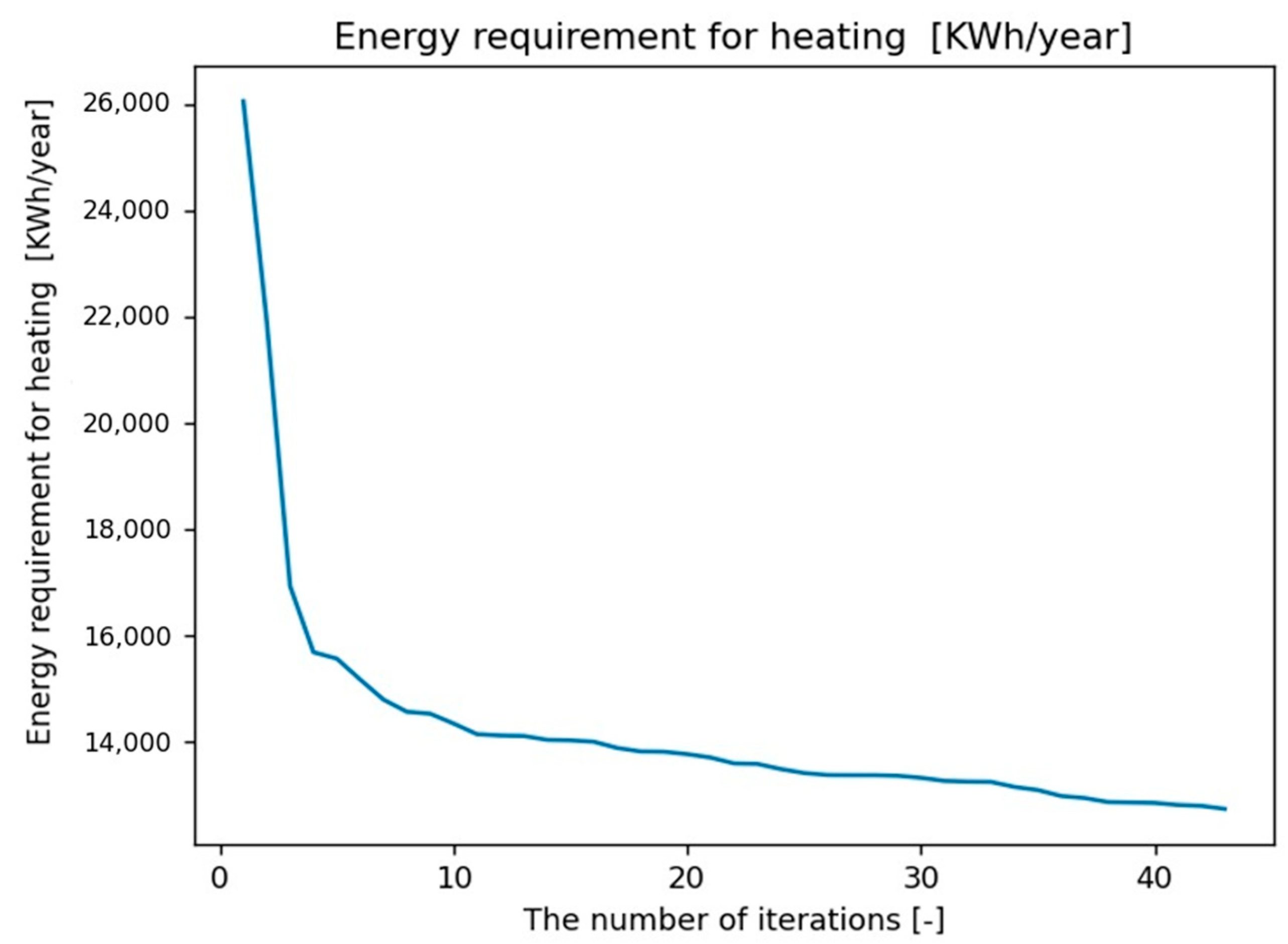
Figure 4 shows the improvement of the energy requirement for heating when the NSGA-II is running. The optimal value of the energy requirement for heating in the case of the insulated building is 12,486.16 kWh/year or 96.05 kWh/m²/year.

The determined energy demand for heating considers the heat losses by infiltration and heat transfer by transmission between the heated space and the outside environment due to temperature differences but does not consider the thermal mass, thermal inputs from solar radiation and internal heat gains from occupants, equipment, and lighting. By using expanded polystyrene, extruded polystyrene, and mineral wool with the thermal characteristics presented in Table 2, and by using triple-insulating windows with U-value of 0.6 W/(m²·K) and a door with an overall heat transfer coefficient of 0.7 W/(m²·K), this energy requirement for heating is reduced by up to 75% compared to the energy requirement for heating obtained in the case of a non-insulated building.

4. Heat Pump Model Optimization

4.1. The Energy Consumption for Domestic Hot Water Preparation

The energy consumption for domestic hot water preparation (Q_am) was computed using the following Equations (30)–(34), while neglecting the losses in the distribution pipes [15].

$$Q_{am}=Q_{ac}+Q_{ac,c }\left[\frac{\mathrm{k}\mathrm{W}\mathrm{h}}{\mathrm{y}\mathrm{e}\mathrm{a}\mathrm{r}}\right]$$

(30)

$$Q_{ac}=\sum _{i=1}^n\rho ·c_w·V_{ac}·\left({\theta }_{ac}-{\theta }_{ar}\right) \left[\frac{\mathrm{k}\mathrm{W}\mathrm{h}}{\mathrm{y}\mathrm{e}\mathrm{a}\mathrm{r}}\right]$$

(31)

$$V_{ac}=\frac{a·N_u}{1000} \left[{\mathrm{m}}^3\right]$$

(32)

$$Q_{ac,c}=\sum \rho ·c_w·V_{ac,c}·\left({\theta }_{ac,c}-{\theta }_{ar}\right) \left[\frac{\mathrm{k}\mathrm{W}\mathrm{h}}{\mathrm{y}\mathrm{e}\mathrm{a}\mathrm{r}}\right]$$

(33)

$$V_{ac,c}=V_{ac}·f_1·f_2-V_{ac} \left[{\mathrm{m}}^3\right]$$

(34)

where Q_ac = the energy required for domestic hot water preparation [kWh/year]; Q_ac,c = the heat losses related to the waste of domestic hot water [kWh/year]; ρ = the density of water [kg/m³]; c_w = the specific heat capacity of liquid water [kJ/(kg·K)]; V_ac = the required volume of domestic hot water for the considered period [m³]; V_ac,c = the volume corresponding to losses and waste of hot water [m³]; θ_ac = the hot water preparation temperature [°C]; θ_ar = the temperature of cold water entering the hot water preparation system [°C]; θ_ac,c = the temperature of supply/use of hot water at the point of consumption [°C]; i = the calculation index for consumer categories [-]; a = the specific demand for domestic hot water at 60 °C [m³]; N_u = number of people [-].

These parameters were considered as stipulated in the national Romanian standards: ρ = 983.2 kg/m³; c = 4.183 kJ/(kg·K); θ_ac = 60 °C; θ_ar = 10 °C; θ_ac,c = 50 °C; f₁ = 1.3 (a coefficient that depends on the type of installation to which the consumption point is connected); f₂ = 1.1 (a coefficient that depends on the technical condition of the armatures where hot water is consumed) [26]. N_u is considered to be 6 and a is considered equal to 50 L/person/day. This value represents the specific hot water consumption needs of one person in a residential buildings, according to [26].

The results were: $Q_{am}=Q_{ac}+Q_{ac,c}=6254.77+2151.64=8406.41 \frac{\mathrm{k}\mathrm{W}\mathrm{h}}{\mathrm{y}\mathrm{e}\mathrm{a}\mathrm{r}}$.

4.2. Heat Pump Simulation

Another important step in the simulation was the selection of the appropriate water–water heat pumps in a closed circuit to guarantee the energy requirements for heating and hot water preparation.

The database used was created based on the RETScreen Expert Software V9.0 information. A total of 345 heat pump models from 30 different manufacturers were compared in Python, considering the following characteristics:

1.

Simulation 1: A maximum cost that can be allocated to heat pumps is set and the heat pumps falling within this cost limit are compared according to the coefficient of performance (COP), thermal load of the capacitor and number of pumps needed to ensure the energy requirements for heating and hot water preparation:

• Criterion 1: Cost _pumps ≤ RON 34,600.
  where RON 34,600 represents the maximum cost that can be allocated to heat pumps. This cost was obtained through a specific market survey. The heat pumps chosen from among 345 heat pumps models after applying the financial criterion are presented in

  Table 3. The heat pumps chosen according to criterion 1.

  Manufacturer	Model	Npumps [-]	Qcpump [kW]	Qopump [kW]	Ppump [kW]	COP [-]	Qc total [kW]	Q0 total [kW]	Ptotal [kW]	Cost [RON]
  Carrier	38YZA01832	3	4.92	2.52	2.40	2.05	14.76	7.56	7.20	34,922
  Econar	GC180	3	4.84	3.42	1.42	3.40	14.52	10.25	4.27	34,354
  FHP	EMO0241CS	3	4.84	3.42	1.42	3.40	14.52	10.25	4.27	34,354
  Hydro Delta	03068WTARHE	1	14.59	9.73	4.86	3.00	14.59	9.73	4.86	34,519
  Trane	GSUF024ICM	3	4.87	3.19	1.68	2.90	14.61	9.57	5.04	34,567
  York International	YZE02411N1VSB16	2	7.30	5.13	2.17	3.36	14.60	10.25	4.35	34,543

  .

• Criterion 2: 1 ≤ N_pumps < 3;

$$N_{pumps}=\frac{Q_{ctotal}}{Q_{cpump}} \text{[-]}$$

(35)

$$Q_{ctotal}=\frac{Q_{heating}+Q_{am}}{h_{pumps}} \left[\mathrm{k}\mathrm{W}\right]$$

(36)

where N_pumps = the number of pumps selected to cover most of the energy requirements for heating and hot water preparation for the studied building [-]; Q_cpump = the thermal load of the capacitor for every studied pump [kW]; Q_ctotal = 14.52 kW represents the thermal load for heating and hot water preparation in the case of our simulation; Q_heating = the energy requirement for heating [kWh/year] (relation 1); Q_am = the energy consumption for domestic hot water preparation [kWh/year] (relation 30); h_pumps = 1512 h/year represents the operating hours of the pump.

To establish h_pumps, it was considered that a heat pump has two cycles per hour, with a twenty-minute off period between cycles. The heat pumps chosen after applying the second criterion were: one heat pump from Hydro Delta manufacturer, model 03068WTARHE and two heat pumps from York International, model YZE02411N1VSB16. These heat pumps are presented in Table 3.

• Criterion 3: COP ≥ 3;

$$COP=\frac{\left|Q_{cpump}\right|}{P_{pump }}=\frac{\left|Q_{cpump}\right|}{\left|Q_{Cpump}\right|-Q_{opump}} \text{[-]}$$

(37)

$$Q_{ototal}=Q_{opump}· N_{pumps} \left[\mathrm{k}\mathrm{W}\right]$$

(38)

$$P_{total}=P_{pump}· N_{pumps} \left[\mathrm{k}\mathrm{W}\right]$$

(39)

where COP = the coefficient of performance [-]; Q_opump = the refrigerating power of the evaporator for every studied pump [kW]; Q_ototal = the total refrigerating power of the evaporators [kW]; P_pump = the power consumed by the compressor for every studied pump [kW]; P_total = the total power consumed by the compressors [kW]. Both heat pumps from the Hydro Delta and York International manufacturers satisfy the third criterion.

• Criterion 4: 14.52 ≤ Q_ctotal ≤ 15.

The heat pumps from the Hydro Delta and York International manufacturers, as presented in Table 3, also satisfy the fourth criterion.

2.

Simulation 2: the heat pumps were compared based on their technical characteristics, as presented at simulation 1 (COP, Q_ctotal, N_pumps), and then it was verified that the selected pumps respect the maximum cost limit. The simulation result shows that two heat pumps with the specifications presented in Figure 5a or one heat pump with the specifications presented in Figure 5b must be installed to guarantee the 14.52 kW thermal load needed for heating and hot water preparation, according to the technical criteria.

Figure 6 shows the characteristics of the heat pumps (two heat pumps from York International and one heat pump from Hydro Delta) that were selected from the Python simulation according to the technical and financial requirements to guarantee the 14.52 kW thermal load needed for heating and hot water preparation.

5. Conclusions

An NSGA-II model was developed in the Pymoo (Multi-Objective Optimization in Python) library and used to find the optimal choice among the following parameters: thermal insulation materials’ conductivities and thicknesses, windows’ overall heat transfer coefficients and total solar energy transmittance and doors’ thermal proprieties. This algorithm finds the materials that ensure the lowest energy requirement for heating, also considering the price restrictions obtained through a specific market survey. A survey was conducted and several price combinations for each configuration (consisting of different pairs of thermal properties) were obtained from the manufacturers’/retailers’ websites. These values were further used to compute the mean values of the prices for each configuration (consisting of different pairs of thermal properties).

The energy requirement for heating before the walls, floor and roof–ceiling thermal insulation was 385.128 kWh/m²/year. This energy requirement for heating considered the heat losses by infiltration and heat transfer by transmission between the heated space and the outside environment due to temperature differences but did not consider the thermal mass, thermal inputs from solar radiation and internal heat gains from occupants, equipment, and lighting. This value was reduced with 75% by using:

• expanded polystyrene with δ_ins1 = 100 mm and λ_ins1 = 0.038 W/(m·K);
• extruded polystyrene with δ_ins2 = 100 mm and λ_ins2 = 0.031 W/(m·K);
• mineral wool δ_ins3 = 200 mm and λ_ins3 = 0.038 W/(m·K);
• triple-glazed IGUs with two 4S glasses and one float glass, separated by argon with U_w = 0.6 W/(m²·K) and g = 0.4;
• one door made of oak covered with stainless steel, with U₂ = 0.7 W/(m²·K).

Additionally, this paper presents the method used in finding the best option from among the available heat pumps that could cover most of the energy requirements for heating and domestic hot water systems, also considering the products’ prices. The heat pumps chosen after applying the technical and financial criteria are one heat pump from Hydro Delta manufacturer, Hudson, FL, USA, model 03068WTARHE and two heat pumps from York International manufacturer, York, PA, USA, model YZE02411N1VSB16.

The result of running the NSGA-II described in this paper shows that this model can be successfully utilized to identify the optimal thermal envelope configuration that will ensure the minimum energy requirement for heating in the case of a residential building, while also considering the price restrictions obtained through a specific market survey.

The presented research is ongoing and, in the future, we will use a complex database including different insulation materials and equipment for the energy calculation of buildings.

References

- European Environment Agency (EEA). Resource Efficiency and Low Carbon Economy—Energy Efficiency. 2019. Available online: https://www.eea.europa.eu/airs/2018/resource-efficiency-and-low-carbon-economy/energy-efficiency (accessed on 7 January 2024).
- Ministry of Regional Development and Public Administration. NZEB Romania: Plan to Increase the Number of Nearly Zero-Energy Buildings. 2014. Available online: https://www.mdlpa.ro/userfiles/metodologie_calcul_performanta_energetica_iulie2014.pdf (accessed on 7 January 2024).
- Building Performance Institute Europe (BPIE). Europe’s Buildings under the Microscope: A Country-by-Country Review of the Energy Performance of Buildings. 2011. Available online: https://bpie.eu/wp-content/uploads/2015/10/HR_EU_B_under_microscope_study.pdf (accessed on 14 January 2024).
- Delgarm, N.; Sajadi, B.; Delgarm, S.; Kowsary. A novel approach for the simulation-based optimization of the buildings energy consumption using NSGA-II: Case study in Iran. Energy Build. 2016, 127, 552–560. [Google Scholar] [CrossRef]
- Niemelä, T.; Kosonen, R.; Jokisalo, J. Cost-effectiveness of energy performance renovation measures in Finnish brick apartment buildings. Energy Build. 2017, 137, 60–75. [Google Scholar] [CrossRef]
- Bingham, R.D.; Agelin-Chaab, M.; Rosen, M.A. Whole building optimization of a residential home with PV and battery storage in The Bahamas. Renew. Energy 2019, 132, 1088–1103. [Google Scholar] [CrossRef]
- Acar, U.; Kaska, O.; Tokgoz, N. Multi-objective optimization of building envelope components at the preliminary design stage for residential buildings in Turkey. J. Build. Eng. 2021, 42, 102499. [Google Scholar] [CrossRef]
- Lapisa, R.; Bozonnet, E.; Salagnac, P.; Abadie, M.O. Optimized design of low-rise commercial buildings under various climates—Energy performance and passive cooling strategies. Build. Environ. 2018, 132, 83–95. [Google Scholar] [CrossRef]
- Kahsay, M.T.; Bitsuamlak, G.T.; Tariku, F. Thermal zoning and window optimization framework for high-rise buildings. Appl. Energy 2021, 292, 116894. [Google Scholar] [CrossRef]
- Wang, R.; Lu, S.; Feng, W. A three-stage optimization methodology for envelope design of passive house considering energy demand, thermal comfort and cost. Energy 2020, 192, 116723. [Google Scholar] [CrossRef]
- Yue, N.; Li, L.; Morandi, A.; Zhao, Y. A metamodel-based multi-objective optimization method to balance thermal comfort and energy efficiency in a campus gymnasium. Energy Build. 2021, 253, 111513. [Google Scholar] [CrossRef]
- Wu, C.; Pan, H.; Luo, Z.; Liu, C.; Huang, H. Multi-objective optimization of residential building energy consumption, daylighting, and thermal comfort based on BO-XGBoost-NSGA-II. Build. Environ. 2024, 254, 111386. [Google Scholar] [CrossRef]
- Nicolae, A.E.; Necula, H.; Carutasiu, B.M. Optimization of energy rehabilitation processes of existing buildings. U.P.B. Sci. Bull. 2023, 85. Available online: https://www.scribd.com/document/404094429/337436568-SR-1907-1-2014-pdf (accessed on 7 January 2024).
- Standard SR1907-1; Heating Installations: Calculation Method. Romanian Standards Association: Bucharest, Romania, 2014.
- Methodology for Calculating the Energy Performance of Buildings, MC001, Part IV—Breviary for Calculating the Energy Performance of Buildings and Apartments. The Official Gazette of Romania. 2010; pp. 00062–00064, Number 243. Available online: https://www.mdlpa.ro/userfiles/reglementari/Domeniul_XXVII/27_11_MC_001_4_5_2009.pdf (accessed on 7 January 2024).
- Normative Regarding the Thermotechnical Calculation of Construction Elements in Contact with the Ground, Indicative C107/5; MTCT: Bucharest, Romania, 2005.
- Deb, K.; Pratap, A.; Agarwal, S.; Meyarivan, T. A Fast and Elitist Multiobjective Genetic Algorithm: NSGA-II. IEEE Trans. Evol. Comput. 2002, 6, 182–197. [Google Scholar] [CrossRef]
- Khan, A.; Baig, A.R. Multi-Objective Feature Subset Selection using Non-dominated Sorting Genetic Algorithm. J. Appl. Res. Technol. 2015, 13, 145–159. [Google Scholar] [CrossRef]
- Mkaouer, M.W.; Kessentini, M. Model Transformation Using Multiobjective Optimization. In Advances in Computers; Hurson, A., Ed.; Elsevier: Amsterdam, The Netherlands, 2014; Volume 92, pp. 161–202. ISBN 978-0-12-420232-0. [Google Scholar]
- Halim, I.; Adhitya, A.; Srinivasan, R. Multi-objective Optimization for Integrated Water Network Synthesis. In Computer Aided Chemical Engineering: Proceedings of the 11th International Symposium on Process Systems Engineering, Singapore, 15–19 July 2012; Karimi, A.I., Srinivasan, R., Eds.; Elsevier: Amsterdam, The Netherlands, 2012; Volume 31, pp. 1432–1436. ISBN 978-0-444-59505-8. [Google Scholar]
- Manne, J.R. Multiobjective Optimization in Water and Environmental Systems Management- MODE Approach. In Handbook of Research on Advanced Computational Techniques for Simulation-Based Engineering; Samui, P., Ed.; Engineering Science Reference: Hershey, PA, USA, 2016; pp. 120–136. ISBN 9781466694798. [Google Scholar]
- Yang, X.-S. Multi-Objective Optimization. In Nature-Inspired Optimization Algorithms; Elsevier: London, UK, 2014; pp. 197–211. ISBN 978-0-12-416743-8. [Google Scholar]
- De Buck, V.; López, C.A.M.; Nimmegeers, P.; Hashem, I.; Van Impe, J. Multi-objective optimisation of chemical processes via improved genetic algorithms: A novel trade-off and termination criterion. In Computer Aided Chemical Engineering, Proceedings of the 29th European Symposium on Computer Aided Process Engineering, Eindhoven, The Netherlands, 16–19 June 2019; Kiss, A.A., Zondervan, E., Lakerveld, R., Özkan, L., Eds.; Elsevier: Amsterdam, The Netherlands, 2019; Volume 46, pp. 613–618. ISBN 978-0-12-818634-3. [Google Scholar]
- Gad, A.F. Practical Computer Vision Applications Using Deep Learning with CNNs; Apress: Berkeley, CA, USA, 2018; ISBN 978-1-4842-4166-0. [Google Scholar]
- Mohanty, R.; Suman, S.; Das, S.K. Modeling the Axial Capacity of Bored Piles Using Multi-Objective Feature Selection, Functional Network and Multivariate Adaptive Regression Spline. In Handbook of Neural Computation; Samui, P., Sekhar, S., Balas, V.E., Eds.; Academic Press: Cambridge, MA, USA, 2017; pp. 295–309. ISBN 978-0-12-811318-9. [Google Scholar]
- Methodology for Calculating the Energy Performance of Buildings, Indicative MC001-2022; MTCT: Bucharest, Romania, 2023.
- Standard SR4839; Heating Installations: Annual Number of Degrees-Days. Romanian Standards Association: Bucharest, Romania, 2014.
- Standard SR1907-2; Heating Installations: Calculation Heat Demand. Conventional Indoor Computing Temperatures. Romanian Standards Association: Bucharest, Romania, 2014.
- Blank, J.; Deb, K. Pymoo: Multi-Objective Optimization in Python. IEEE Access 2020, 8, 89497–89509. [Google Scholar] [CrossRef]
- Bailey, E.T.; Caldas, L. Operative generative design using non-dominated sorting genetic algorithm II (NSGA-II). Autom. Constr. 2023, 155, 105026. [Google Scholar] [CrossRef]
- Normative Regarding the Thermotechnical Calculation of Building Construction Elements, Indicative C107/3; MTCT: Bucharest, Romania, 2005.
- Pramanik, S.; Setua, S.K. A steady state Genetic Algorithm for Multiple Sequence Alignment. In Proceedings of the International Conference on Advances in Computing, Communications and Informatics (ICACCI), Delhi, India, 24–27 September 2014. [Google Scholar]
- Lozano, M.; Herrera, F.; Cano, J. Replacement strategies to preserve useful diversity in steady-state genetic algorithms. Inf. Sci. 2008, 178, 4421–4433. [Google Scholar] [CrossRef]
- Zeng, F.; Low, M.Y.H.; Decraene, J.; Zhou, S.; Cai, W. Self-Adaptive Mechanism for Multi-objective Evolutionary Algorithms. In Proceeding of the International Multi Conference of Engineers and Computer Scientists, Hong Kong, China, 17–19 March 2010. [Google Scholar]
- Deb, K.; Agrawal, S. A Niched-Penalty Approach for Constraint Handling in Genetic Algorithms. In Artificial Neural Nets and Genetic Algorithms: Proceedings of the International Conference in Slovenia, Portorož, Slovenia, 6–9 April 1999; Springer: Vienna, Austria, 1999. [Google Scholar]
- Fanggidae, A.; Prasetyo, M.I.C.; Polly, Y.T.; Boru, M. New Approach of Self-Adaptive Simulated Binary Crossover-Elitism in Genetic Algorithms for Numerical Function Optimization. Int. J. Intell. Syst. Appl. Eng. 2024, 12, 174–183. [Google Scholar]
- Deb, K.; Sindhya, K.; Okabe, T. Self-adaptive simulated binary crossover for real-parameter optimization. In Proceedings of the 9th Annual Conference on Genetic and Evolutionary Computation, London, UK, 7–11 July 2007. [Google Scholar]
Figure 1.
Non-dominated Sorting Genetic Algorithm II.
Figure 2.
The construction materials.