

Use of CAMS near Real-Time Aerosols in the HARMONIE-AROME NWP Model

1
Agencia Estatal de Meteorología (AEMET), 8 (Ciudad Universitaria), 28071 Madrid, Spain
2
Irish Meteorological Service (Met Éireann), 65/67 Glasnevin Hill, D09 Y921 Dublin, Ireland
3
Finnish Meteorological Institute (FMI), P.O. Box 503, FI-00101 Helsinki, Finland
*
Author to whom correspondence should be addressed.
Meteorology 2024, 3(2), 161-190; https://0-doi-org.brum.beds.ac.uk/10.3390/meteorology3020008
Submission received: 29 February 2024
/
Revised: 9 April 2024
/
Accepted: 18 April 2024
/
Published: 26 April 2024
Abstract
:Near real-time aerosol fields from the Copernicus Atmospheric Monitoring Services (CAMS), operated by the European Centre for Medium-Range Weather Forecasts (ECMWF), are configured for use in the HARMONIE-AROME Numerical Weather Prediction model. Aerosol mass mixing ratios from CAMS are introduced in the model through the first guess and lateral boundary conditions and are advected by the model dynamics. The cloud droplet number concentration is obtained from the aerosol fields and used by the microphysics and radiation schemes in the model. The results show an improvement in radiation, especially during desert dust events (differences of nearly 100 W/m2 are obtained). There is also a change in precipitation patterns, with an increase in precipitation, mainly during heavy precipitation events. A reduction in spurious fog is also found. In addition, the use of the CAMS near real-time aerosols results in an improvement in global shortwave radiation forecasts when the clouds are thick due to an improved estimation of the cloud droplet number concentration.
1. Introduction
Aerosols influence weather and climate directly by scattering and absorbing solar and terrestrial radiation. They act as nuclei for cloud liquid droplet and ice crystal formation, which impacts clouds and precipitation. Clouds largely control the surface radiation balance, whose changes influence near-surface temperature and humidity. Changes in cloud optical properties due to aerosols further modify atmospheric radiative transfer.
The particle number concentration (PNC) in the atmosphere can have high variability throughout the year. Measurements of PNC in the Baltic Sea found daily mean concentrations varying from 40 cm−3 in August 2008 to 12,500 cm−3 in April 2008 [1]. For example, the burning of fossil fuels for heating increases the PNC during winter. In general, the origin of an air mass shows up in the composition of aerosols.
During wildfire, volcanic eruption, and desert dust intrusion events, the mass of various aerosols in the air can increase locally by orders of magnitude compared to the average. Remote transfer, by atmospheric flow, may carry aerosols over thousands of kilometers and high up in the atmosphere, as recently demonstrated by [2]. The common way of representing aerosols, by monthly climatological fields of aerosol optical depth (AOD) in limited area numerical weather prediction (NWP) models such as [3] and only accounting for aerosols in the radiation parameterizations, is clearly inadequate [4] in such cases.
The cloud droplet number concentration (CDNC) in clouds shows considerable variability. Measurements of CDNC in fog can be between 10 and 500 cm−3 [5]. When considering all supersaturation values and fog types, the typical range can be estimated to be roughly between 15 and 250 cm−3 [6]. Aircraft observations estimated that typical CDNC values are between 100 cm−3 and 200 cm−3 for marine and continental regions [7], but the value can be in the range of 1–500 cm−3 [8].
Global and regional models of atmospheric composition integrated into weather models like IFS-AER [9], ICON-ART [10], and WRF-CHEM [11,12] (see also an early review by [13]), as well as coupled atmospheric transport models like MOCAGE [14] or SILAM [15,16], are capable of monitoring and forecasting atmospheric aerosol concentrations on a daily basis. These models comprise advanced data on aerosol sources, parameterization of physicochemical processes to simulate aerosol evolution, and handling of aerosol transport and scavenging. In addition, they may utilize the assimilation of satellite-based observational aerosol data to determine the initial state of each forecast. Limited area NWP models that cannot afford the simulation of complicated aerosol dynamics within the weather forecast can rely on global atmospheric composition forecasts as a source of near real-time aerosol information. The task remaining for the weather models is to utilize these aerosol data for cloud microphysics and radiative transfer parameterizations. This approach is being developed within the HARMONIE-AROME weather model.
In this study, we report on the use of Copernicus Atmosphere Monitoring Service (CAMS) global aerosol forecasts within HARMONIE-AROME [3]. HARMONIE-AROME is a canonical model configuration of the shared ACCORD NWP system [17] for short-range operational weather forecasting. CAMS, operated by the European Centre for Medium-Range Weather Forecasts (ECMWF), provides aerosol fields in near real-time. The atmospheric composition modeling used in the Integrated Forecasting System (IFS) and operationally at the ECMWF is described in [9,18].
The aim of this paper is to document the suggested usage of CAMS aerosol data within HARMONIE-AROME cycle 46h1 (release version 1 of cycle 46). We focus on how aerosols impact cloud-precipitation microphysics within the ICE3/OCND2 microphysics scheme that interacts with the default radiation scheme. Both schemes were documented in [3]. We also checked the impact of our developments on fog, as previous work has also used the CAMS aerosol configuration for fog studies [6]. Aerosol mass mixing ratio (MMR) fields, obtained from CAMS during the initialization of each HARMONIE-AROME weather forecast, are advected by the dynamics of the model and updated at the horizontal boundaries during the forecast. The key variable, estimated from aerosol MMR fields for cloud microphysics parameterizations, is the CDNC at every grid point and every time step. The CDNC is also used to obtain the effective radius of cloud liquid droplets for the radiation scheme. For radiative transfer parameterizations, aerosol MMRs are combined with prescribed mass extinction coefficients to determine runtime AOD fields.
The paper is organized as follows. In Section 2, we describe the aerosol species obtained from CAMS. Section 3 details the processes concerning the advection and removal of aerosols. Section 4 is dedicated to the calculation of the aerosol PNC, as well as the derivation of the cloud condensation nuclei (CCN) and CDNC of particles from aerosol MMR fields. A short description of the cloud microphysics parameterizations that use the CDNC is included in Section 5, while Section 6 summarizes the use of aerosols in the radiation scheme. In Section 7, we analyze the impact of NRT aerosols through a series of test cases that focus on precipitation, radiation, and fog. In Section 8, we present verification results, and in Section 9, the radiation forecast is analyzed using the clear sky index. The results are discussed in Section 10. Conclusions and ideas for future work are provided in Section 11.
2. Description of CAMS Aerosol Types
The aerosol outputs from the IFS model are released as CAMS Global near real-time data. The horizontal resolution of the data is approximately 40 km (T511L60) and is available at 3-h intervals. The system only produces two 5-day forecasts per day, at 00 UTC and 12 UTC. In [9], the different species used in CAMS are described, as well as the processes for the production and removal of aerosols. For HARMONIE-AROME, we use seven aerosol types from CAMS: sea salt (SS), desert dust (DD), organic matter (OM), black carbon (BC), sulfates (SU), nitrates (NI), and ammonium (AM). Relevant information about the aerosol types is detailed in this section for completeness. Each aerosol type can be described by several aerosol species. In the case of OM and BC, there are two species for each with hygroscopic characteristics (hydrophobic and hydrophilic). For SS and DD, three bin sizes are considered, while two bin sizes are considered for NI. Therefore, a total of 14 aerosol species (14 different fields) are taken into account. The parameters of the log-normal aerosol size distributions, the aerosol size bin limits, and the mass densities for each of the aerosol species can be found in Table 1.
2.1. Sea Salt
The most abundant aerosol in the IFS model is SS. The production of SS depends not only on the value of the mean wind speed over the sea but also on the gustiness ([20]). SS is the most hygroscopic of the aerosols considered [19] and is typically larger than other hygroscopic aerosols. These facts, together with the production of large SS particles over the sea, make it the most relevant aerosol in cloud development in maritime air. Three SS aerosol species are used with the radius limits provided in [9]. In addition, two log-normal size distributions are used to characterize SS. The "film drop" mode is used for the first bin and is described by one log-normal size distribution. A second log-normal distribution is used for the "jet" and "spume drop" modes that describe the remaining two species.
2.2. Desert Dust
Mineral dust production takes place in arid regions. As in the case of SS emission, dust production is also wind-dependent [20]. DD is composed of quartz and clay and can act as ice nuclei. It has a strong impact on solar radiation on a global scale, and the impact is significant at locations near mineral dust sources during dust storm events [21]. DD is described by three species or size bins: fine, coarse, and super-coarse, but a single log-normal size distribution is used for each bin.
2.3. Organic Matter
OM is characterized by a large number of individual compounds with different hygroscopic properties. Water-soluble OM has an influence on CDNC, while the majority of semi-volatile OM has no influence [22]. In CAMS, OM is described by three modes: WASO (water soluble), INSO (insoluble), and SOOT (as in soot), with , , and , respectively. These modes have different densities and size distribution parameters. For simplicity reasons, in HARMONIE-AROME, only one value for mass and size distribution parameters is considered for hydrophilic and hydrophobic OM. In the CAMS model, the hydrophobic component is transformed into a hydrophilic component once the aerosol is emitted [9], but this mechanism has not been introduced in our scheme yet.
2.4. Black Carbon
Black carbon strongly absorbs radiation at infrared and visible wavelengths. An estimate of its global radiative force is around 0.4 W m−2 [23]. BC has a short lifetime in the atmosphere, and its sources are mainly anthropogenic. Two species representing BC are used in CAMS: hydrophobic and hydrophilic. As in the case of OM, the hydrophobic component transforms into a hydrophilic component in the CAMS model once it is emitted, but this is also not yet implemented in our scheme.
2.5. Sulfates
Sulfates originate from sulfur emissions of different origins: natural sources, such as volcanic or biogenic emissions, fuel combustion, and biomass burning. The emission of sulfates is related to economic and industrial development [24]. The number of components in the atmosphere that contain sulfur is high, but here we assume that the chemical composition is that of ammonium sulfate (NH4)2SO4. This assumption restricts the values of the particle density and the hygroscopic parameter.
2.6. Nitrates and Ammonium
The decrease in anthropogenic emissions of sulfur dioxide [24] has increased the relative importance of nitrates and ammonium. Coarse-mode nitrate particles are produced from heterogeneous reactions over DD and SS particles [25]. The values of the size distribution parameters for the CAMS nitrate and ammonium species are shown in Table 1.
3. Advection and Removal of Aerosols
The scheme described in this paper is introduced into cycle 46h1 of HARMONIE-AROME. MMR aerosol fields from CAMS are interpolated to the model grid and included in the first guess and lateral boundary condition (LBC) files, together with atmospheric fields from the high-resolution (HRES) IFS model. As the aerosol fields are available every 3 h, and hourly atmospheric fields are produced from the HRES model, time interpolation of the aerosol fields is carried out so that they are available in the hourly LBCs. Once the model reads the aerosol fields from the first guess, they are advected by the model dynamics.
Aerosol emissions or chemical processes have not been parametrized in HARMONIE-AROME, but aerosol removal processes have been introduced. These aerosol-removal parameterizations are wet deposition and sedimentation and follow [9,26], respectively. The dry deposition of aerosols has been parametrized and tested, but when activated, it was found to result in a strong reduction in aerosols in the lower layers of the atmosphere for long forecast lengths. Given that there is no aerosol production in HARMONIE-AROME for the time being, the cases were run without dry deposition. Nevertheless, these processes are briefly described in the following subsections.
3.1. Wet Deposition
In HARMONIE-AROME, wet deposition (or scavenging) for stratiform and convective precipitation is not treated separately. Wet deposition works on all of the aerosol species considered except hydrophobic BC and OM in the case of “inside cloud” scavenging.
The scavenging rate (unit: s−1) inside the cloud, or rainout, for an aerosol species, , is provided by the following expression:
where (Table 2) is the fraction of aerosol included in the droplets, is the cloud fraction at the model level k, and is the rate of conversion of cloud water to rainwater that is given as follows:
where and are the precipitation fluxes for rain and snow at level k, and are the precipitation fluxes for rain and snow at level , is the air density, is the model level height, and and are the ice and liquid water mass mixing ratios, respectively. The fraction of aerosols in the aqueous phase is taken from [9] with the values provided in Table 2. However, for hydrophilic species, is obtained by the fraction of activated nuclei, with the values shown in Table 2 being the maximum permitted.
In the case of below-cloud wet deposition or washout, the scavenging rate, , is obtained as follows:
where and are the rain and snow fluxes at the model level k as before, and and are the liquid water and ice densities. and are the efficiencies of rain and snow at washing out aerosols, with values of 0.001 and 0.01, respectively. and are the assumed mean radius of rain droplets and snow crystals, with a value of used for both.
3.2. Aerosol Sedimentation
The parameterization of sedimentation follows [26]. This is only applied to coarser modes of SS and DD and is an important removal mechanism for these aerosol species. The tendency of the MMR of an aerosol species due to sedimentation is obtained as follows:
where is the MMR of an aerosol species (s), z is the height, and is the settling velocity, which, in this case, is provided by Stoke’s law:
where is the mean radius of an aerosol bin, is the particle density, is the dynamic (absolute) viscosity of the air, and is the Cunningham correction that takes into account the dependency of viscosity on air pressure and temperature.
4. Calculation of the Particle Number Concentration (PNC), Cloud Condensation Nuclei (CCN), and Cloud Droplet Number Concentration (CDNC)
The total number concentration of the aerosols is calculated from the MMR fields using the aerosol log-normal size distribution for each aerosol species and atmospheric variables in a similar way to [27,28]. Because the same size distribution is used for DD and SS aerosol species, we need to use truncated distributions so that the values of the distributions are zero outside the bin limits. The MMR of an aerosol species () is provided by the following:
where s refers to the aerosol species, is the PNC of species s, is the density of the solute, is the particle density (see Table 1), and is the mean value of the cubic radius. Rearranging Equation (6), we obtain the following:
The mean value of the cubic radius is calculated from the size distribution of each aerosol species, a log-normal size distribution () provided by the following:
where is the radius of the particle, is the geometric standard deviation, and is the “number mode radius” of the size distribution (the parameters of the size distribution for each aerosol type are found in Table 1).
We obtain the mean cubic radius using the log-normal size distribution in Equation (8), integrating between zero and infinity, see [29]:
However, this is not the expression for the mean cubic radius to be used in Equation (7). In order to take the bin limits of the different species into account, it is convenient to derive the expressions for the mean cubic radius and the particle number concentration directly from the integration formulas (a detailed calculation is shown in Appendix A).
where is a correction factor depending on the bin limits, and the functions and are provided by Equations (A2) and (A6), respectively.
Substituting Equation (10) into Equation (7), we obtain the following expression for the PNC of an aerosol species with the bin limits taken into account. The value of for each aerosol bin and the rest of the values of the size distribution and mass density required for this equation are provided in Table 1.
4.1. Cloud Condensation Nuclei (CCN) and Cloud Droplet Number Concentration (CDNC)
The cloud condensation nuclei (CCN) concentration is obtained from the particle concentration and the ambient supersaturation of the model in a similar way as is described in [27]. Under saturated conditions, hygroscopic particles bigger than a given radius are activated. The calculation of that minimum radius of activation, and the number of nuclei activated (), is described in this subsection.
As mentioned before, the activation of aerosol particles depends on ambient supersaturation and critical supersaturation. The Köhler theory (1936) describes the equilibrium stage of a droplet in a saturated environment based on the physicochemical properties of the aerosols. According to [30], there are two approaches to describe the influence of chemical composition on water activity, one of which is a parameter that describes the equilibrium interaction of particles with water vapor [31]. One is the osmotic coefficient reference model, and the other uses an effective hygroscopicity parameter. The second approach is known as the -Köhler theory [19]. The first approach can be easily applied to inorganic compounds. However, for more complex organic compounds, the -Kohler theory is more convenient as it uses a single parameter, the hygroscopic parameter (), to describe water activity. Therefore, this is the method that we use for all aerosol species. Hygroscopic species have values greater than 0.5, with values close to 1 for most hygroscopic species and with as an upper limit. For moderately hygroscopic species, the values are between [19]. The hygroscopic parameters are listed in Table 1.
We consider that the volume of dry solute () is much smaller than the volume of water in the droplet (), i.e., , so that the Köhler equation for the saturation ratio at equilibrium () can be simplified and written as follows:
where is the droplet radius and A is defined as follows:
where is the surface tension of the water, is the gas constant of water vapor, T the temperature, and the water density. Parameter B in Equation (12) is obtained as follows:
where is the hygroscopic parameter obtained from [19], and is the radius of the aerosol particle.
The simplified expression of Equation (12) allows us to obtain the minimum radius of an aerosol particle activated in a supersaturated environment, where the maximum value of Equation (12) provides the critical saturation. The corresponding radius of a cloud droplet at the critical saturation is obtained as follows:
The critical supersaturation, , for an aerosol particle of radius is obtained as follows:
All particles whose critical supersaturation, , is equal to or higher than the ambient supersaturation () are considered to be activated. By setting , we obtain the minimum radius () of an aerosol species for which the aerosol can become activated. This minimum radius is equal to the following:
The number of activated condensation nuclei or CCNs for a given aerosol type can be determined by calculating the integral of the size distribution function, Equation (8), between and the upper bin limit, . Making use of Equations (A2)–(A4), we obtain the following:
where is the lower bin limit, and the function is provided by Equation (A2).
Although most of cloud droplets grow as a result of the activation process, large aerosols with a high enough hygroscopic factor can grow to reach diameters in the range of those of cloud droplets without being activated [32]. Those small droplets, which do not become CCNs, are not taken into account in the calculation of CDNC. Processes in which the CDNC is important require larger droplets. Only activated CCNs are considered. The total concentration of CCNs is the sum of CCNs for all SS, SU, hydrophilic BC and OM, nitrates, and ammonia.
There is no straightforward relationship between CCN and CDNC in the atmosphere. Ref. [33], as part of the third Pallas Cloud Experiment (PaCE-3), found a good correlation between CDNC and CCN. Ref. [34] showed a positive correlation between and using measurements from the RICO and PASE projects, with negative correlations for large/intermediate size cloud droplets, although it must be noted that the values were obtained for a fixed supersaturation of . Therefore, a direct equivalence between the CDNC () and the CCN, , is considered. Also, a minimum value of 10 cm−3 is considered for both and , given that there is no aerosol generation in the model, and the removal of aerosols could produce values that are too low and unrealistic. Furthermore, a minimum value of 2 μm is used for the mean cloud droplet radius to avoid unrealistic cases where cloud water is shared by a large number of tiny droplets. Whenever the mean cloud droplet radius, calculated for a given cloud water amount, is lower than the minimum radius, the CDNC will be reduced until the mean radius is equal to the minimum value (this is checked at every time step of the model integration).
4.2. Ambient Supersaturation
Ambient supersaturation depends on vertical velocity, but the presence of coarse SS reduces supersaturation. As has been shown, ambient supersaturation provides the number of droplets inside clouds. Given the ambient vapor pressure, , and the equilibrium water vapor pressure at saturation, , the ambient saturation ratio is defined as follows:
The activation of cloud nuclei is determined by the ambient supersaturation ratio, , and the critical supersaturation of each particle.
The HARMONIE-AROME model adjusts the humidity variables at every time step. This causes supersaturation to reduce considerably in the adjustment. Because of this, the activation of the condensation nuclei is much lower than expected. In order to obtain realistic values for the CCN, it is necessary to set a minimum value for supersaturation inside clouds in order to activate the condensation nuclei. By analyzing rainfall events in East Asia, ref. [35] observed that the in-cloud supersaturation experienced by removing aerosols had an average value of , ranging from to . In the case of fog, ref. [32] applied a method using aerosol and cloud droplet measurements, estimating that supersaturation was between 0.01% and 0.05% for different fog cases. These values agree with the maximum supersaturation of 0.049% found by [36] in radiation fog with non-gradient turbulent mixing. Ref. [37] obtained supersaturation values through aerosol and droplet measurements at the SIRTA observatory in a suburb of Paris and derived a median critical supersaturation of 0.043% for fog cases during the winters of 2010–2013. Based on these results, we consider a minimum value of 0.05% for supersaturation at the lowest level of the model. Minimum supersaturation increases linearly to 0.08% at the surface up to an arbitrary height of 100 m, remaining constant above that height. This minimum supersaturation is described in Equation (21).
where is the minimum supersaturation, is the supersaturation at the surface, , z is the height of the model level, and H is the reference height of 100 m.
The dependence of supersaturation on the vertical velocity has also been parameterized following [38]. The rate of change in supersaturation due to vertical ascents is obtained as follows:
where w is the vertical velocity, t is the time, is the ambient supersaturation, T is the temperature, is the latent heat of condensation, is the specific heat of dry air at constant pressure, is the molecular weight of water, is the mean molecular weight of dry air, and is the specific ideal gas constant.
It is known that the presence of large particles of SS reduces ambient supersaturation due to competition for water vapor [39]. Over the sea, [40] found values of effective supersaturation of , assuming = 1.1. Taking this into account, it has been assumed that large SS particles, those with sizes greater than 0.5 μm (jet drop mode and spume drop mode in Table 1), are activated in clouds. It is also assumed that they stay at equilibrium with the surrounding air and that they remove an amount of water vapor provided by condensation on the droplets by diffusion during each time step, thus reducing supersaturation. In order to estimate the rate of change in supersaturation by the presence of coarse SS particles, we consider a mean radius for an aerosol particle of μm, for which the droplet radius () is provided by Equation (15). The estimation of the rate of change in supersaturation by the presence of coarse SS particles is carried out as follows:
where is the diffusion coefficient, is the SS hygroscopic parameter, and is the coarse SS number concentration for which a maximum of 10 cm−3 is considered. Only a reduction of 0.03· 10−2 in the supersaturation is allowed due to the presence of coarse SS. The derivation of Equation (23) can be found in Appendix B.
Finally, the expression for ambient supersaturation is given as follows:
where is the model time step. The value for ambient supersaturation obtained by Equation (24) and is substituted into Equation (17) to calculate the number of activated nuclei (Equation (18)).
Figure 1 shows a cross-section of condensation nuclei, supersaturation, and the CDNC provided by the model on the 16 February 2020, with the details specified in the caption of the figure. It must be noted that where updrafts are stronger, supersaturation is higher. This gives rise to an increment in CDNC.
5. Description of the Microphysical Parameterizations in HARMONIE-AROME
The introduction of NRT aerosols affects several processes in microphysics parameterizations through modifying the CDNC. By default, the CDNC in cycle 46h1 in HARMONIE-AROME has a vertical dependence on height. A reference concentration of 250 cm−3 is considered at a pressure of 1000 hPa. The concentration increases linearly with pressure at a rate of , where P is the pressure at each model level. A reduction is applied to CDNC at the lowest model level, where the concentration is multiplied by a factor of . This was carried out to improve the forecasting of low visibility and fog.
The microphysics parametrization scheme in the HARMONIE-AROME model is called ICE3 [3]. A particular configuration named OCND2 is activated [41]. In this scheme, some of the processes already depend on a prescribed value of the CDNC, so significant modifications of the microphysics parameterizations is not needed as it only required a substitution of the prescribed value of CDNC by that obtained from NRT aerosols. The four processes that depend on CDNC are as follows: autoconversion, as long as Kogan parameterization ([42]) is activated, cloud droplet sedimentation, accretion of cloud liquid, and riming of snow by cloud droplets.
5.1. Autoconversion
Autoconversion is the process of forming drizzle through the self-collection of cloud droplets. It is responsible for the initiation of precipitation. Autoconversion in HARMONIE-AROME within OCND2 uses Kogan parameterization described in [42]. The rain MMR rate is obtained as follows:
where is the rain MMR, is the cloud water MMR, and is the CDNC.
Autoconversion is enhanced when the CDNC is reduced with respect to the reference value in the model. As supersaturation depends strongly on vertical velocity, the higher supersaturation in the updrafts increases the CDNC. Given the dependence of autoconversion on , the increment in CDNC reduces its effects. This changes the precipitation patterns. In order to avoid drizzle in situations where the cloud droplets are too small to initiate self-collection, parameterization is activated only when the mean radius of the cloud droplets is larger than 20 micrometers.
5.2. Accretion of Cloud Droplets
Through the collection of cloud droplets, raindrops grow. Accretion contributes to increasing the intensity of precipitation. The rain MMR rate is obtained as follows:
where is the rain droplet diameter, is the number of rain droplets per unit volume (which is considered to be constant), is the rain droplet terminal velocity that depends on the rain droplet diameter, is the rain droplet size distribution represented by the exponential law, and is the collision efficiency of rain droplets with cloud droplets. Only the collision efficiency is affected by the introduction of NRT aerosols. In the parametrization of accretion, the collision efficiency, based on [43,44], is defined as follows:
where is the mean radius of the cloud droplets in micrometers, and it itself is obtained as follows:
where is the density of the air, and is the water density. The modification of CDNC () results in a change in the mean radius and collision efficiency. The collision efficiency decreases with CDNC and increases with cloud water content. In general, an increase in precipitation is found when NRT aerosols are used, especially during strong precipitation events. This occurs because the CDNC is reduced in most cases with respect to the default configuration, which increases the collision efficiency.
5.3. Cloud Droplet Sedimentation
Cloud droplet sedimentation is an important process in fog development and in the evolution of cloud thickness. The cloud water MMR rate of sedimentation is obtained as follows:
where is the cloud water MMR, and is the mixing ratio sedimentation flux (in kg m−2 s−1) obtained as follows:
where is the terminal velocity of the cloud droplets obtained in Appendix C.
The modification of CDNC is expected to have an important effect on the Stokes velocity. In general, a reduction in compared with the reference values increases the terminal velocity, , and sedimentation. For a comprehensive study of the different cloud droplet configurations in the model, see [45].
5.4. Riming of Snow
The riming of snow is parameterized as in [46]. However, the OCND2 option considers the dependence of the collision efficiency of aggregates and cloud droplets, with cloud droplet size as defined in [47]. The collision efficiency, , is calculated as follows:
where is the Stokes number, which depends on the terminal velocity of the cloud droplets obtained as follows:
For this parameterization, the terminal velocity of the droplets () is obtained using an analytical formula which considers, not only the Stokes regime for low values of the Reynolds number (), but also a regime with intermediate values of .
The collision efficiency has a maximum value when the terminal velocity of the cloud droplets is 0.5 m/s. This corresponds approximately with the volume mean radius () considered as the limit of the Stokes regime, which is 65.0 μm. The cloud water content and CDNC determine the volume mean radius of the cloud droplets.
6. Impact on Radiation
The use of NRT aerosols in the model modifies radiative transfer because of the extinction caused by different aerosol species (direct effect), while the use of CDNC from aerosols modifies the effective radius of cloud droplets (indirect effect).
The default radiation parameterizations in HARMONIE-AROME ([3,48]) are based on an ECMWF radiation scheme (ECMWF model cycle 25r) [49]. To characterize aerosol interaction in the SW and LW radiation schemes, monthly climatologies of vertically integrated AOD at 550 nm (AOD550) for six aerosol species are used, further denoted as the Tegen climatology [50]. These species are land, sea, urban, and desert aerosols. Prescribed background values are assumed for missing tropospheric components and stratospheric volcanic ash and sulphates. The increase in the total AOD550 due to the assumed background values is approximately 0.08 (unitless). The AOD550s are vertically distributed using exponential vertical profiles, as described in [51], with modifications suggested by [52]. In addition to AOD550, the inherent aerosol optical properties (AIOPs) include single-scattering albedos and asymmetry factors, which are prescribed for the six aerosol species. Spectral distributions of each AIOP are also prescribed.
In earlier studies, the use of improved AOD550 climatologies demonstrated quite a limited impact on HARMONIE-AROME results [53,54]. The use of NRT aerosols, instead of climatologies, provides more realistic data and permits us to calculate the AOD at every model level directly from the MMRs of the different CAMS aerosol species. To convert the MMRs to AODs, aerosol mass extinction coefficients at 550 nm, provided by CAMS, are applied following the method of [52]. The prescribed values of the single-scattering albedo and asymmetry factor and the spectral distributions of all AIOPs were not modified when introducing CAMS MMRs. Also, all cloud optical property parameterizations [3] remained unchanged when aerosol MMRs were introduced.
The AODs of CAMS aerosol species are combined with Tegen aerosol species as follows: the AOD of the Tegen land aerosol is obtained from CAMS organic matter, sulphate, nitrate, and ammonium aerosols, and the sea species from the sum of the AODs of the three CAMS sea salt size bins. The Tegen desert dust is calculated from the three desert dust size bins from CAMS, and the Tegen urban aerosol is calculated from CAMS black carbon. Additional background aerosols are not assumed in the troposphere or stratosphere. This is expected to lead to a negligible reduction in the total AOD, except in the case of volcanic events. In this version, nitrates and ammonia are not used because mass extinction coefficients are not available. The lack of these two species causes a small increase in the surface-level (clear sky) SW radiation output of the model.
HARMONIE-AROME radiation parameterization results were shown to be sensitive to the assumed cloud droplet and ice crystal sizes [55]. There are several possibilities for calculating the effective radius, , of cloud liquid droplets. We modified the default method, based on [56], to take into account aerosol-based CDNC. By default, is related to CDNC as follows:
where is the cloud water content MMR, is the water density, is the assumed CDNC, and is a variable called the spectral dispersion, with over sea and over land. When NRT aerosols are considered, the calculation of the effective radius is modified to take the cloud droplet distribution provided by Equation (A14) into account. can thus be written as follows:
where and are the shape parameters of the cloud droplet size distribution. Given that and over sea, and and over land, comparing Equations (34) and (35), we obtain the corresponding values of over sea and over land when the cloud droplet size distribution is used. While the value of over sea is very similar to the value used by default in the model, over land the difference is higher. We did not modify the parameterization of the ice particle equivalent radius due to aerosols.
7. Test Cases
Several test cases have been considered to show the impact of using NRT aerosols in cycle 46h1 of HARMONIE-AROME. The domain considered for the experiments over the Iberian Peninsula extends from 30 to 50 degrees North and from 20 degrees West to approximately 10 degrees East. It covers the entire Iberian Peninsula, the south of France, and the northwestern part of Africa. The grid is 1152 longitude points times 864 latitude points, and the grid spacing is 2.5 km, with 65 vertical levels and a time step of 60 s. Results are also shown for experiments run over a domain covering Ireland, the UK, and part of Northern France. The horizontal grid spacing, vertical resolution, and time-step are the same as that of the Iberian setup.
In the examples shown, two experiments are defined. A reference experiment (REFERENCE) is configured with default values of parameters in HARMONIE-AROME cycle 46h1. As mentioned in Section 5, by default in HARMONIE-AROME, the CDNC has a vertical dependence on height and increases linearly with the pressure at a rate of , with P representing the pressure of the model level. The Tegen aerosol climatology is used in the radiation scheme. In experiments that use NRT aerosols (CAMSNRT), the CDNC is derived from model aerosol fields and atmospheric variables, as described in Section 4. A minimum value of 10 cm−3 is used for CDNC. The AOD is obtained from the aerosol fields and their mass extinction parameters. The experiments are run with a cold start unless otherwise specified.
7.1. Warm Rain Case
To illustrate the impact of the use of calculating the CDNC from NRT aerosols on warm rain, a frontal precipitation case, which occurred on the 16 February 2020, affecting the NW of the Iberian peninsula, has been selected. During the first half of the day, warm rain from stratiform clouds fell over Galicia and the NW of Portugal. The processes of autoconversion, sedimentation, and accretion of cloud droplets were responsible for the formation and evolution of the rain (see Section 5).
In Figure 2, instantaneous precipitation over Galicia at 12 UTC is shown for the two experiments (REFERENCE and CAMSNRT). The black line depicts the location of the cross-section plots shown in Figure 3, where the rainfall intensity is plotted. It can be seen that the introduction of NRT aerosols modifies the structure of the precipitation field. In the CAMSNRT experiment, precipitation is less homogeneously distributed, and maximum precipitation values are higher even though the zones of maximum precipitation coincide with those of the REFERENCE experiment.
Figure 1 (top left) shows the cross-section of the total condensation nuclei. A layer of particles with concentrations of over 2000 particles per cm3 can be seen at a height of just over 1000 m over land. Above this layer, the air is cleaner, with values of around 200 cm−3. Higher supersaturation in the updrafts (Figure 1, top right) causes an increase in the CDNC (Figure 1, bottom left). This allows higher values of cloud water content (Figure 1, bottom right) because the autoconversion and collision of cloud droplets are less efficient with a larger number of droplets. Once the vertical velocity decreases, the higher amount of cloud water leads to an increase in the intensity of the precipitation relative to the reference experiment.
7.2. Snow Case
The riming of snowflakes by cloud droplets, described in Section 5, contributes to an increase in precipitation in the form of snow. As the parameterization of this process depends on CDNC, the number of aerosols has an impact on the intensity of the snow. On 23 February 2023, after the passage of a frontal system, atmospheric instability increased with northerly winds producing precipitation in the form of snow over the northern part of the Iberian Peninsula. Its intensity for the REFERENCE and CAMSNRT experiments at 12 UTC, over an area covering the northern plateau of the Iberian Peninsula, is shown in Figure 4. The intensity of the snow is greater in the case of CAMSNRT, especially over mountainous regions. There are some differences in its distribution with areas where the snowfall is lower for CAMSNRT.
Figure 5 shows cross-sections of snow intensity and cloud water content. An increase in the intensity of snowfall is observed in the CAMSNRT experiment compared to the REFERENCE experiment, while the cloud water content is lower than expected because the increase in snow intensity is at its expense.
Figure 6 shows the cross-section of the total condensation nuclei, the supersaturation, and the CDNC for the CAMSNRT experiment. In this case, the air is very clean, as the maximum number of condensation nuclei is around 300 particles per cm3. Under such conditions, the CDNC is also very low, which helps to increase the riming of the snow. The CDNC from the REFERENCE experiment is also plotted to show the difference compared to the CAMSNRT experiment. In this case, the CDNC for the REFERENCE experiment is around 20 times the value of that for CAMSNRT.
7.3. Radiation Cases
Three test cases have been chosen to show the impact of NRT aerosols on radiation. Daily global radiation plots for these cases are shown in Figure 7 and compared with observations.
We selected a dust event that occurred on 31 March 2021 over the Iberian peninsula where Saharan dust reduced SW radiation by nearly 100 W/m2 at some stations during the day. The accumulated global radiation over 24 h for the two experiments is shown in Figure 8. The day was characterized by clear skies over most of the Iberian area.
As can be seen in Figure 7 (left), the global radiation forecast by the REFERENCE experiment was overestimated, while the introduction of NRT aerosols reduced global radiation to values similar to those observed.
In order to demonstrate the impact of aerosols on solar irradiance, two further test cases were considered: one for a cloudy day and another for a mainly clear day. They were run for the Iberian domain with one week of warm-up.
Figure 9 shows the accumulated global radiation over the Iberian domain on 22 October 2020 for the two experiments (REFERENCE and CAMSNRT) for the cloudy case. Clearly, there is an increase in global radiation when NRT aerosols are introduced. We found that cloud cover was lower for the CAMSNRT experiment compared to the REFERENCE, but the main cause of the difference in global radiation was the higher transparency of the clouds due to a higher effective droplet radius when NRT aerosols were considered.
In the central image of Figure 7, the REFERENCE experiment shows an underestimation of global radiation compared to observations, while the CAMSNRT results match the observed radiation much better, with a slight overestimation at midday.
For the clear sky case, we selected 12 October 2020. We found that the global radiation under clear sky conditions is overestimated when NRT aerosols are introduced. One possible reason for this could be the omission of certain aerosol species (nitrates and ammonia) in the radiation parameterizations. Figure 10 shows the accumulated global radiation over 24 h for the two experiments for the Iberian domain.
7.4. Fog Case
In order to characterize fog, we used the diagnosed visibility, but we did not study the impact on visibility itself. The parameterization of visibility in HARMONIE-AROME takes the five prognostic hydrometeors of HARMONIE-AROME into account, including 2 m relative humidity, 2 m temperature, and the climatological cloud condensation nuclei distribution. The calculation of 2 m visibility is described in [57].
Cloud droplet sedimentation is one of the processes that take part in the evolution and dissipation of fog. As mentioned in Section 5, sedimentation depends on the CDNC. Two cases of fog in the Irish domain are included here. The first is for 14 April 2021, Figure 11, when a large area of high pressure covered Ireland. Cycle 43h1.1 of HARMONIE-AROME was operational at the time and over-predicted fog for this event. As for the previous examples, both a REFERENCE and a CAMSNRT experiment were run for this case. A large fog bank can be seen in the Irish Sea in the REFERENCE experiment, which was not present in observations. This fog bank is not present in the CAMSNRT results. As the use of CAMSNRT aerosols results in less fog in some cases, there was a concern that using CAMSNRT aerosols could result in a general underprediction of fog. The second example shown is of a case for 13 May 2023, Figure 12, when fog over the Irish Sea extended during the day and encroached on the east of the country around the Greater Dublin Area. In this example, some of the erroneous fog over Ireland at 00 Z is not present in the CAMSNRT run, while the fog bank over the Irish Sea is retained at 00 Z and 06 Z.
8. Verification Results
Point verification was run for the REFERENCE and CAMSNRT experiments for two periods over the Iberian domain. The Autumn period was from 1–30 October 2020, and the Spring period was from 1–30 May 2021. Figure 13 shows the equitable threat score (ETS) for 12 h precipitation for both periods. It clearly shows that the skill for high precipitation values improves in the case where NRT aerosols were configured. High precipitation events are less frequent, and they are likely to be affected by the double penalty problem. This means ETS values are reduced for those. With NRT aerosols, the general increase in forecast precipitation seems to have more of an impact on high precipitation cases.
Figure 14 shows scatter plots of the 24 h precipitation for the spring period. There are only five events for which the observations were over 80 mm. Although the number is too small to be significant, the CAMSNRT experiment produced higher precipitation compared with REFERENCE. In the interval between 40 mm and 80 mm, there is an underestimation of the precipitation in both experiments, but more points are closer to the diagonal in the CAMSNRT plot.
In Table 3, point verification results for several variables are shown. In general, when NRT aerosols are introduced, 2 m temperature values are higher, with a small improvement in the standard deviation (STDV) of the biases. This can be due to an increase in radiation, given that the clouds are more transparent. The surface pressure is reduced, although the bias is not always better. Meanwhile, the 10 m wind speed increases, resulting in a higher bias, with similar values for the STDV. The 2 m relative humidity decreases and is worse for both periods. Only the standard deviation is improved in spring. The cloud cover is reduced, especially in the autumn period. There is an increase in the 24 h accumulated precipitation, for which the STDV also improves.
9. Clear Sky Index
Global horizontal irradiance (GHI), also referred to as “global radiation”, provides an objective and quantitative measure for evaluating cloud forecasts during the daytime. GHI is the shortwave irradiance integrated over all downward directions and wavelengths in the solar spectrum received by a horizontal surface of unit area. Furthermore, non-dimensional indices for solar energy resource assessment have been developed in recent years and decades and are very useful. One such index is the clear sky index (CSI), which is the GHI divided by the theoretical GHI during clear sky conditions. In this paper, we use the theoretical GHI clear sky model of [58,59], which includes coefficients that account for variable integrated atmospheric water vapor, aerosols, and ozone. We assumed an atmosphere with an integrated water vapor load of 2.5 g cm−2, which is a typical load for a mid-latitude location like Ireland.
Figure 15 shows 1D histograms of observed versus modeled CSI for the REFERENCE (Tegen) and CAMSNRT experiments. Observations from 20 sites around Ireland were used, along with corresponding model data for the same locations. The results for the 2-week spring period (8–22 May 2020) are shown on the left, with the autumn period (1–14 November 2019) shown on the right. A clear overestimation of low CSI in the REFERENCE HARMONIE-AROME can be seen in both seasons, consistent with an overestimation of cloud condensate in the thickest clouds (not shown but confirmed by comparison with an MSG cloud water path product available from KNMI). This overestimation of low CSI is not present when CAMS NRT aerosols are used.
Figure 16 shows 2D histograms of observed versus modeled CSIs, using data similar to that of Figure 15. The results for the 2-week spring period are shown in the first row, with the autumn period shown in the bottom row. REFERENCE is on the left and CAMSNRT on the right. A clear overestimation of low CSI in HARMONIE-AROME can be seen on the left panels, as in the case of Figure 15. In the case of CAMSNRT, a general overestimation is seen in global SW radiation, as can be seen with more values above the dashed x–y line in the figure, meaning that, in general, the CSI is higher in the model than observed. The overestimation in global SW radiation is also shown in Figure 17, where positive and negative biases are plotted on the positive axis to highlight whether an experiment results in more positive or negative biases overall. These biases were calculated for the same 20 stations as before. It is clear that in the REFERENCE experiments (both spring and autumn; left figures) there are negative biases overall, with positive biases overall when CAMSNRT aerosols are used (right figures), and slightly smaller biases when CAMSNRT aerosols are used.
10. Discussion
In this article, we have shown how HARMONIE-AROME forecasts change when NRT aerosols from CAMS are introduced into cloud-precipitation microphysics and radiation parameterizations. Mass mixing ratios of the hygroscopic aerosol species are used to calculate the cloud droplet number concentration for every grid point in the three-dimensional model grid. The calculated values of CDNC are introduced in the microphysical processes instead of the prescribed values. The calculation of the CDNC from aerosol MMR is based on the Köhler theory and depends on the value of supersaturation. The aerosol MMR fields are used directly in the radiation scheme to obtain aerosol optical density at every model level. Cloud liquid droplet effective radii are derived from the aerosol-based CDNC for estimation of the indirect aerosol effect on shortwave radiation. It must be pointed out that the microphysical parameterizations already depended on CDNC. Thus, modification of the subroutines of the OCND2 scheme was not required.
Calculation of the CDNC from the aerosol fields and atmospheric conditions, such as the humidity and vertical velocity, permits a more realistic representation of the transport of cloud water. The dependence of the parameterizations of the autoconversion and collision of cloud droplets on CDNC is fundamental for modifying the precipitation intensity and patterns. The verification results show that rain is better forecast in general, especially with high precipitation values that used to be underestimated. The increase in precipitation when using NRT aerosols seems to be related to an increase in the collision efficiency. This may be due to an increase in the cloud water available in the clouds or to a decrease in the CDNC compared to the reference scheme. Sensitivity tests are required to understand and tune model variables in order to reduce overestimation. For snowfall, it was shown that the introduction of NRT-based CDNC also produces an increase in precipitation in the form of snow. This can be explained by the dependence of riming on CDNC, resulting in a reduction in the cloud water content.
The HARMONIE-AROME model occasionally produces spurious fog. The reason for this is not totally clear, but the sedimentation process, which depends on the CDNC, is important for the formation and evolution of fog. For the cases shown, the spurious fog predicted by the model is not present when NRT aerosols are employed.
One of the highest impacts of the inclusion of NRT aerosols in the model occurs in the forecast of solar radiation during dust intrusion episodes. In such cases, aerosol concentrations in the air may increase by orders of magnitude locally compared to the average grid-scale climatological dust concentrations. Downwelling SW radiation at the surface is then much better forecast with NRT aerosols than with default monthly climatologies. Radiation fluxes are also mostly improved under cloudy conditions. On average, cloud cover and cloud condensate are slightly reduced, which makes clouds optically more transparent. Clouds also become more transparent to SW radiation because the prescribed CDNC is replaced by values derived from NRT aerosol distribution, which seems to improve the representation of the effective radius of the cloud liquid droplets. However, under partially cloudy conditions, an overestimation of the shortwave radiation is observed. This overestimation is expected to be reduced once the nitrate and ammonium species are introduced into the radiation scheme but preliminary tests have shown that this may not be sufficient.
Although the introduction of NRT aerosols in the HARMONIE-AROME model has resulted in a significant advancement towards better representation of atmospheric composition, for particular cases, further development is still required. For cloud-precipitation microphysics parameterizations, such development includes the transformation of hydrophobic OM and BC into hydrophilic species. The calculation and use of ice nuclei, especially those derived from DD fields, is expected to be important for the treatment of ice clouds. Inclusion of SS and DD emissions may also be relevant for limited-area high-resolution NWP models like HARMONIE-AROME. Together with emission treatment, dry deposition parameterization should be developed. With the alternative radiation schemes that will be fully available in the coming versions of the ACRANEB [60,61] and ecRad [62] models, it will become possible to combine the updated humidity-dependent aerosol optical properties of all available species (including nitrate and ammonium) over the full spectrum of SW and LW radiation with NRT, or updated climatological, aerosol MMR data. There is also room for an improved estimation of cloud particle effective size for radiation parameterizations based on aerosol data.
The use of NRT aerosols in HARMONIE-AROME results in an increase in the required computational resources. The addition of 14 3D fields to the files means an increase in storage memory requirements. Also, during the execution of the model, the memory requested is higher, and more HPC nodes may be required if the same execution time is to be achieved. In the case where the same computational resources are used, the execution time for a 24 h forecast is longer when NRT aerosols are used compared with the execution of the model for the same date and forecast length with the default configuration. This increase in execution time is a drawback regarding the use the NRT aerosols operationally.
11. Conclusions
In this paper, we have shown the methods used to introduce NRT aerosols from CAMS in the HARMONIE-AROME model and how the MMR and CDNC, calculated from those, are used by this model. We have shown the impact on different meteorological phenomena. The structure of the precipitation field was modified and a positive impact was found in the case of high precipitation events. The spurious fog that sometimes appears in HARMONIE-AROME forecasts was reduced when NRT aerosols were considered. A big impact was also found for dust events, and solar radiation under cloudy conditions was forecast much better.
Nevertheless, more studies are still required. Long period verification is recommended to fully demonstrate the quality of the improvements on the forecasts. The calculation of supersaturation can be improved by adding an extra term for infrared radiative cooling. Dry deposition can be activated once sea salt and desert dust emissions are parameterized. The calculation of ice nuclei from NRT aerosols is also possible and will have an impact on the cold processes of the model.
Author Contributions
D.M.P. wrote the paper with input from E.G., P.M. and L.R.; D.M.P. ran most of the experiments but the fog cases and CSI results were carried out by E.G.; D.M.P. and L.R. developed the parts of the NWP code for implementing CAMSNRT aerosols into HARMONIE-AROME. All authors have read and agreed to the published version of the manuscript.
Funding
This research received no external funding.
Data Availability Statement
The original contributions presented in the study are included in the article, further inquiries can be directed to the corresponding author.
Acknowledgments
We thank our colleagues within the ACCORD consortium for active and stimulating collaboration. We also thank the referees for their useful comments and suggestions.
Conflicts of Interest
The authors declare no conflicts of interest.
Abbreviations
The following abbreviations are used in this manuscript:
| AOD | Aerosol Optical Depth. |
| BC | Black Carbon. |
| CAMS | Copernicus Atmospheric Monitoring Services. |
| CCN | Cloud Condensation Nuclei. |
| CDNC | Cloud Droplet Number Concentration. |
| CSI | Clear Sky Index |
| DD | Desert Dust. |
| IFN | Ice Forming Nuclei. |
| IFS | Integrated Forecast System. |
| ECMWF | European Centre for Medium-Range Weather Forecasts. |
| LAM | Limited Area Model. |
| LBC | Lateral Boundary Conditions. |
| MMR | Mass Mixing Ratio. |
| NRT | Near Real-Time. |
| OM | Organic Matter. |
| PNC | Particle Number Concentration. |
| SS | Sea Salt. |
| SU | Sulphate. |
Appendix A. Correction of the Cubic Radius of the Log Normal Size Distribution
The cubic radius of an aerosol species whose size distribution is log-normal is calculated taking the bin limits into account. The log-normal distribution () is obtained as follows:
where is the particle radius, is the “number mode radius”, and is the geometric standard deviation of the log-normal size distribution for the aerosol species. The integral of the log normal size distribution is the error function (erf).
We define the following parameters:
The expression for the third moment of size distribution is provided as follows:
We define the following parameters:
Finally, we obtain the expression for the corrected mean cubic radius as follows (this is only for the particles whose radii are within those bin limits):
Appendix B. Estimation of Correction of Supersaturation by the Presence of Large Sea Salt Particles
The ambient supersaturation is obtained as follows:
where is the water vapor mass mixing ratio, P is the air pressure, is the saturation vapor pressure, and is the ratio between the gas constant for dry air and the gas constant for water vapor. We approximated this assuming . The variation of the supersaturation is provided as follows:
where we consider that the variation of the water vapor is due to the loss or gain of vapor by the cloud droplets, where is the mass of a droplet and the number of droplets. We also consider that with the density of the air and the gas constant for dry air. Given the growth of a droplet by diffusion ([63])
where is the ambient water vapor pressure, and is the equilibrium water vapor pressure at the surface of a droplet of radius from around an aerosol SS particle considered to be a sphere of radius . Substituting Equation (A11) and making use of the Köhler Equations (12) and (14), we obtain the following:
Appendix C. Cloud Droplet Terminal Velocity Calculation
In HARMONIE-AROME, the cloud droplet size spectrum is represented by the generalized gamma distribution:
where is the gamma function, is the cloud droplet diameter, is the slope parameter, and and are the distribution shape parameters. The shape parameters considered in HARMONIE-AROME are , over land, and , over sea. The parameter is obtained from the predicted moment of the distribution (i.e., the mass mixing ratio):
where is the liquid water content, is the water density, and is the density of the air. In the parameterization of sedimentation, the CDNC and the shape parameters of the cloud droplet size distribution (Equation (A14)) are used. Sedimentation depends on the terminal velocity of the cloud droplets, and this terminal velocity is proportional to the square of the radius in the Stokes regime [64]. We also follow [65]. We can obtain the mean value of the terminal velocity for a group of droplets described by a generalized gamma distribution. First of all, the stokes terminal velocity of a single droplet is obtained as follows:
where is the droplet radius, g is the acceleration due to gravity, and is the dynamic viscosity, which is considered to be constant ( Pa s). We consider a term expressing the dependence of the terminal velocity with the air density, , [66], where is the air density in conditions of 293.15 K, 101,325 Pa, and 50% humidity. In the calculation of the mean value of the stokes terminal velocity, the air density is considered to be negligible compared with the density of water, . The terminal velocity of a collection of cloud droplets is obtained as follows:
Considering a generalized gamma distribution, we finally obtain the following:
In the HARMONIE-AROME model, a correction term for very small droplets is also considered. This is the Cunningham correction factor [64], which influences the droplet terminal velocity. Its application is not critical for general behavior.
References
- Byčenkienė, S.; Ulevicius, V.; Prokopčiuk, N.; Jasinevičienė, D. Observations of the aerosol particle number concentration in the marine boundary layer over the south-eastern Baltic Sea. Oceanologia 2013, 55, 573–597. [Google Scholar] [CrossRef]
- Meinander, O.; Kouznetsov, R.; Uppstu, A.; Sofiev, M.; Kaakinen, A.; Salminen, J.; Rontu, L.; Welti, A.; Francis, D.; Piedehierro, A.A.; et al. African dust transport and deposition modelling verified through a citizen science campaign in Finland. Sci. Rep. 2023, 13, 21379. [Google Scholar] [CrossRef] [PubMed]
- Bengtsson, L.; Andrae, U.; Aspelien, T.; Batrak, Y.; Calvo, J.; de Rooy, W.; Gleeson, E.; Hansen-Sass, B.; Homleid, M.; Hortal, M.; et al. The HARMONIE–AROME model configuration in the ALADIN–HIRLAM NWP system. Mon. Weather. Rev. 2017, 145, 1919–1935. [Google Scholar] [CrossRef]
- Rontu, L.; Gleeson, E.; Martin Perez, D.; Pagh Nielsen, K.; Toll, V. Sensitivity of radiative fluxes to aerosols in the ALADIN-HIRLAM numerical weather prediction system. Atmosphere 2020, 11, 205. [Google Scholar] [CrossRef]
- Mazoyer, M.; Burnet, F.; Denjean, C. Experimental study on the evolution of droplet size distribution during the fog life cycle. Atmos. Chem. Phys. 2022, 22, 11305–11321. [Google Scholar] [CrossRef]
- Maalampi, P. Studying the Effect of a New Aerosol Option on HARMONIE-AROME Sea Fog Forecasts. Master’s Thesis, University of Helsinki, Helsinki, Finland, 2024. Available online: http://urn.fi/URN:NBN:fi:hulib-202403111471 (accessed on 17 April 2024).
- Gultepe, I.; Isaac, G. Aircraft observations of cloud droplet number concentration: Implications for climate studies. Q. J. R. Meteorol. Soc. 2004, 130, 2377–2390. [Google Scholar] [CrossRef]
- Gultepe, I.; Isaac, G. Scale effects on averaging of cloud droplet and aerosol number concentrations: Observations and models. J. Clim. 1999, 12, 1268–1279. [Google Scholar] [CrossRef]
- Rémy, S.; Kipling, Z.; Flemming, J.; Boucher, O.; Nabat, P.; Michou, M.; Bozzo, A.; Ades, M.; Huijnen, V.; Benedetti, A.; et al. Description and evaluation of the tropospheric aerosol scheme in the European Centre for Medium-Range Weather Forecasts (ECMWF) Integrated Forecasting System (IFS-AER, cycle 45R1). Geosci. Model Dev. 2019, 12, 4627–4659. [Google Scholar] [CrossRef]
- Rieger, D.; Bangert, M.; Bischoff-Gauss, I.; Förstner, J.; Lundgren, K.; Reinert, D.; Schröter, J.; Vogel, H.; Zängl, G.; Ruhnke, R.; et al. ICON–ART 1.0—A new online-coupled model system from the global to regional scale. Geosci. Model Dev. 2015, 8, 1659–1676. [Google Scholar] [CrossRef]
- WRF-Chem. Weather Research and Forecasting Model Coupled to Chemistry. Available online: https://ruc.noaa.gov/wrf/wrf-chem/ (accessed on 19 April 2024).
- Grell, G.A.; Peckham, S.E.; Schmitz, R.; McKeen, S.A.; Frost, G.; Skamarock, W.C.; Eder, B. Fully coupled “online” chemistry within the WRF model. Atmos. Environ. 2005, 39, 6957–6975. [Google Scholar] [CrossRef]
- Baklanov, A.; Schlünzen, K.; Suppan, P.; Baldasano, J.; Brunner, D.; Aksoyoglu, S.; Carmichael, G.; Douros, J.; Flemming, J.; Forkel, R.; et al. Online coupled regional meteorology chemistry models in Europe: Current status and prospects. Atmos. Chem. Phys. 2014, 14, 317–398. [Google Scholar] [CrossRef]
- El Amraoui, L.; Plu, M.; Guidard, V.; Cornut, F.; Bacles, M. A Pre-Operational System Based on the Assimilation of MODIS Aerosol Optical Depth in the MOCAGE Chemical Transport Model. Remote. Sens. 2022, 14, 1949. [Google Scholar] [CrossRef]
- SILAM. System for Integrated modeLling of Atmospheric coMposition. Available online: https://silam.fmi.fi (accessed on 19 April 2024).
- Sofiev, M.; Vankevich, R.; Lotjonen, M.; Prank, M.; Petukhov, V.; Ermakova, T.; Koskinen, J.; Kukkonen, J. An operational system for the assimilation of the satellite information on wild-land fires for the needs of air quality modelling and forecasting. Atmos. Chem. Phys. 2009, 9, 6833–6847. [Google Scholar] [CrossRef]
- ACCORD. A Consortium for COnvection-Scale Modelling Research and Development. Available online: https://www.umr-cnrm.fr/accord/ (accessed on 19 April 2024).
- Rémy, S.; Kipling, Z.; Huijnen, V.; Flemming, J.; Nabat, P.; Michou, M.; Ades, M.; Engelen, R.; Peuch, V.H. Description and evaluation of the tropospheric aerosol scheme in the Integrated Forecasting System (IFS-AER, cycle 47R1) of ECMWF. Geosci. Model Dev. 2022, 15, 4881–4912. [Google Scholar] [CrossRef]
- Petters, M.; Kreidenweis, S. A single parameter representation of hygroscopic growth and cloud condensation nucleus activity. Atmos. Chem. Phys. 2007, 7, 1961–1971. [Google Scholar] [CrossRef]
- Morcrette, J.J.; Beljaars, A.; Benedetti, A.; Jones, L.; Boucher, O. Sea-salt and dust aerosols in the ECMWF IFS model. Geophys. Res. Lett. 2008, 35, L24813. [Google Scholar] [CrossRef]
- García, R.; García, O.; Cuevas, E.; Cachorro, V.; Romero-Campos, P.; Ramos, R.; De Frutos, A. Solar radiation measurements compared to simulations at the BSRN Izaña station. Mineral dust radiative forcing and efficiency study. J. Geophys. Res. Atmos. 2014, 119, 179–194. [Google Scholar] [CrossRef]
- Anttila, T.; Kerminen, V.M. Influence of organic compounds on the cloud droplet activation: A model investigation considering the volatility, water solubility, and surface activity of organic matter. J. Geophys. Res. Atmos. 2002, 107, AAC-12. [Google Scholar] [CrossRef]
- Reddington, C.L.; McMeeking, G.; Mann, G.W.; Coe, H.; Frontoso, M.G.; Liu, D.; Flynn, M.; Spracklen, D.V.; Carslaw, K.S. The mass and number size distributions of black carbon aerosol over Europe. Atmos. Chem. Phys. 2013, 13, 4917–4939. [Google Scholar] [CrossRef]
- Berglen, T.F.; Myhre, G.; Isaksen, I.S.; Vestreng, V.; Smith, S.J. Sulphate trends in Europe: Are we able to model the recent observed decrease. Tellus Chem. Phys. Meteorol. 2007, 59, 773–786. [Google Scholar] [CrossRef]
- Hauglustaine, D.A.; Balkanski, Y.; Schulz, M. A global model simulation of present and future nitrate aerosols and their direct radiative forcing of climate. Atmos. Chem. Phys. 2014, 14, 11031–11063. [Google Scholar] [CrossRef]
- Morcrette, J.J.; Boucher, O.; Jones, L.; Salmond, D.; Bechtold, P.; Beljaars, A.; Benedetti, A.; Bonet, A.; Kaiser, J.; Razinger, M.; et al. Aerosol analysis and forecast in the European Centre for medium-range weather forecasts integrated forecast system: Forward modeling. J. Geophys. Res. Atmos. 2009, 114, D06206. [Google Scholar] [CrossRef]
- Abdul-Razzak, H.; Ghan, S.J.; Rivera-Carpio, C. A parameterization of aerosol activation: 1. Single aerosol type. J. Geophys. Res. Atmos. 1998, 103, 6123–6131. [Google Scholar] [CrossRef]
- Abdul-Razzak, H.; Ghan, S.J. A parameterization of aerosol activation: 2. Multiple aerosol types. J. Geophys. Res. Atmos. 2000, 105, 6837–6844. [Google Scholar] [CrossRef]
- Tulet, P.; Crassier, V.; Cousin, F.; Suhre, K.; Rosset, R. ORILAM, a three-moment lognormal aerosol scheme for mesoscale atmospheric model: Online coupling into the Meso-NH-C model and validation on the Escompte campaign. J. Geophys. Res. Atmos. 2005, 110, D18201. [Google Scholar] [CrossRef]
- Reutter, P.; Su, H.; Trentmann, J.; Simmel, M.; Rose, D.; Gunthe, S.; Wernli, H.; Andreae, M.; Pöschl, U. Aerosol-and updraft-limited regimes of cloud droplet formation: Influence of particle number, size and hygroscopicity on the activation of cloud condensation nuclei (CCN). Atmos. Chem. Phys. 2009, 9, 7067–7080. [Google Scholar] [CrossRef]
- Kreidenweis, S.; Koehler, K.; DeMott, P.; Prenni, A.; Carrico, C.; Ervens, B. Water activity and activation diameters from hygroscopicity data-Part I: Theory and application to inorganic salts. Atmos. Chem. Phys. 2005, 5, 1357–1370. [Google Scholar] [CrossRef]
- Shen, C.; Zhao, C.; Ma, N.; Tao, J.; Zhao, G.; Yu, Y.; Kuang, Y. Method to estimate water vapor supersaturation in the ambient activation process using aerosol and droplet measurement data. J. Geophys. Res. Atmos. 2018, 123, 10–606. [Google Scholar] [CrossRef]
- Anttila, T.; Brus, D.; Jaatinen, A.; Hyvärinen, A.P.; Kivekäs, N.; Romakkaniemi, S.; Komppula, M.; Lihavainen, H. Relationships between particles, cloud condensation nuclei and cloud droplet activation during the third Pallas Cloud Experiment. Atmos. Chem. Phys. 2012, 12, 11435–11450. [Google Scholar] [CrossRef]
- Hudson, J.G.; Noble, S. CCN and cloud droplet concentrations at a remote ocean site. Geophys. Res. Lett. 2009, 36, L13812. [Google Scholar] [CrossRef]
- Moteki, N.; Mori, T.; Matsui, H.; Ohata, S. Observational constraint of in-cloud supersaturation for simulations of aerosol rainout in atmospheric models. NPJ Clim. Atmos. Sci. 2019, 2, 1–11. [Google Scholar] [CrossRef]
- Gerber, H. Supersaturation and droplet spectral evolution in fog. J. Atmos. Sci. 1991, 48, 2569–2588. [Google Scholar] [CrossRef]
- Mazoyer, M.; Burnet, F.; Roberts, G.; Haeffelin, M.; Dupont, J.C.; Elias, T. Experimental study of the aerosol impact on fog microphysics. In Atmos. Chem. Phys. 2019, 19, 4323–4344. [Google Scholar] [CrossRef]
- Khvorostyanov, V.I.; Curry, J.A. Thermodynamics, Kinetics, and Microphysics of Clouds; Cambridge University Press: Cambridge, UK, 2014. [Google Scholar]
- Ghan, S.J.; Guzman, G.; Abdul-Razzak, H. Competition between sea salt and sulfate particles as cloud condensation nuclei. J. Atmos. Sci. 1998, 55, 3340–3347. [Google Scholar] [CrossRef]
- Duplessis, P.; Bhatia, S.; Hartery, S.; Wheeler, M.J.; Chang, R.Y.W. Microphysics of aerosol, fog and droplet residuals on the Canadian Atlantic coast. Atmos. Res. 2021, 264, 105859. [Google Scholar] [CrossRef]
- Müller, M.; Homleid, M.; Ivarsson, K.I.; Køltzow, M.A.; Lindskog, M.; Midtbø, K.H.; Andrae, U.; Aspelien, T.; Berggren, L.; Bjørge, D.; et al. AROME-MetCoOp: A Nordic Convective-Scale Operational Weather Prediction Model. Weather. Forecast. 2017, 32, 609–627. [Google Scholar] [CrossRef]
- Khairoutdinov, M.; Kogan, Y. A new cloud physics parameterization in a large-eddy simulation model of marine stratocumulus. Mon. Weather. Rev. 2000, 128, 229–243. [Google Scholar] [CrossRef]
- Yau, M.K.; Rogers, R.R. A Short Course in Cloud Physics; Elsevier: Amsterdam, The Netherlands, 1996. [Google Scholar]
- Ivarsson, K.I. Decription of the OCND2-option in the ICE3 clouds and stratiform condensation scheme in AROME. In ALADIN-HIRLAM Newsletter No. 5; 2015; pp. 83–87. Available online: https://www.umr-cnrm.fr/aladin/IMG/pdf/nl5.pdf (accessed on 22 April 2024).
- Contreras Osorio, S.; Martín Pérez, D.; Ivarsson, K.I.; Nielsen, K.P.; de Rooy, W.C.; Gleeson, E.; McAufield, E. Impact of the Microphysics in HARMONIE-AROME on Fog. Atmosphere 2022, 13, 2127. [Google Scholar] [CrossRef]
- Farley, R.D.; Price, P.E.; Orville, H.D.; Hirsch, J.H. On the numerical simulation of graupel/hail initiation via the riming of snow in bulk water microphysical cloud models. J. Appl. Meteorol. 1989, 28, 1128–1131. [Google Scholar] [CrossRef]
- Lohmann, U. Can anthropogenic aerosols decrease the snowfall rate? J. Atmos. Sci. 2004, 61, 2457–2468. [Google Scholar] [CrossRef]
- Gleeson, E.; Toll, V.; Nielsen, K.P.; Rontu, L.; Mašek, J. Effects of aerosols on clear-sky solar radiation in the ALADIN-HIRLAM NWP system. Atmos. Chem. Phys. 2016, 16, 5933–5948. [Google Scholar] [CrossRef]
- ECMWF. IFS documentation – Cy47r3 part IV: Physical processes, Chapter 2. Eur. Cent.-Medium-Range Weather. Forecast. 2020, 1, 7–33. Available online: https://www.ecmwf.int/sites/default/files/elibrary/2021/20198-ifs-documentation-cy47r3-part-vi-physical-processes.pdf (accessed on 25 February 2024).
- Tegen, I.; Hollrig, P.; Chin, M.; Fung, I.; Jacob, D.; Penner, J. Contribution of different aerosol species to the global aerosol extinction optical thickness: Estimates from model results. J. Geophys. Res. Atmos. 1997, 102, 23895–23915. [Google Scholar] [CrossRef]
- Tanré, D.; Geleyn, J.; Slingo, J. First results of the introduction of an advanced aerosol-radiation interaction in the ECMWF low resolution global model. Aerosols Their Clim. Eff. 1984, 133, 177. [Google Scholar]
- Bozzo, A.; Benedetti, A.; Flemming, J.; Kipling, Z.; Rémy, S. An aerosol climatology for global models based on the tropospheric aerosol scheme in the Integrated Forecasting System of ECMWF. Geosci. Model Dev. 2020, 13, 1007–1034. [Google Scholar] [CrossRef]
- Toll, V.; Gleeson, E.; Nielsen, K.; Männik, A.; Mašek, J.; Rontu, L.; Post, P. Impacts of the direct radiative effect of aerosols in numerical weather prediction over Europe using the ALADIN-HIRLAM NWP system. Atmos. Res. 2016, 172, 163–173. [Google Scholar] [CrossRef]
- Rontu, L.; Pietikäinen, J.P.; Martin Perez, D. Renewal of aerosol data for ALADIN-HIRLAM radiation parametrizations. Adv. Sci. Res. 2019, 16, 129–136. [Google Scholar] [CrossRef]
- Nielsen, K.P.; Gleeson, E.; Rontu, L. Radiation sensitivity tests of the HARMONIE 37h1 NWP model. Geosci. Model Dev. 2014, 7, 1433–1449. [Google Scholar] [CrossRef]
- Martin, G.; Johnson, D.; Spice, A. The measurement and parameterization of effective radius of droplets in warm stratocumulus clouds. J. Atmos. Sci. 1994, 51, 1823–1842. [Google Scholar] [CrossRef]
- Petersen, C.; Nielsen, N.W. Diagnosis of Visibility in DMI-HIRLAM; DMI Scientific Report 00-11. 2000. Available online: https://www.dmi.dk/fileadmin/Rapporter/SR/sr00-11.pdf (accessed on 22 April 2024).
- Savijärvi, H. Fast radiation parameterization schemes for mesoscale and short-range forecast models. J. Appl. Meteorol. Climatol. 1990, 29, 437–447. [Google Scholar] [CrossRef]
- Gleeson, E.; Nielsen, K.; Toll, V.; Rontu, L.; Whelan, E. Shortwave Radiation Experiments in HARMONIE. Tests of the cloud inhomogeneity factor and a new cloud liquid optical property scheme compared to observations. Aladin-Hirlam Newsl. 2015, 5, 92–106. [Google Scholar]
- Mašek, J.; Geleyn, J.F.; Brožková, R.; Giot, O.; Achom, H.O.; Kuma, P. Single interval shortwave radiation scheme with parameterized optical saturation and spectral overlaps. Q. J. R. Meteorol. Soc. 2016, 142, 304–326. [Google Scholar] [CrossRef]
- Geleyn, J.F.; Mašek, J.; Brožková, R.; Kuma, P.; Degrauwe, D.; Hello, G.; Pristov, N. Single interval longwave radiation scheme based on the net exchanged rate decomposition with bracketing. Q. J. R. Meteorol. Soc. 2017, 143, 1313–1335. [Google Scholar] [CrossRef]
- Hogan, R.J.; Bozzo, A. A Flexible and Efficient Radiation Scheme for the ECMWF Model. J. Adv. Model. Earth Syst. 2018, 10, 1990–2008. [Google Scholar] [CrossRef]
- Mordy, W. Computations of the growth by condensation of a population of cloud droplets. Tellus 1959, 11, 16–44. [Google Scholar] [CrossRef]
- Pruppacher, H.R.; Klett, J.D. Microphysics of Clouds and Precipitation; Springer: Dordrecht, The Netherlands, 1997. [Google Scholar]
- Beard, K. Terminal velocity adjustment for cloud and precipitation drops aloft. J. Atmos. Sci. 1976, 33, 851–864. [Google Scholar] [CrossRef]
- Foote, G.B.; Du Toit, P. Terminal velocity of raindrops aloft. J. Appl. Meteorol. 1969, 8, 249–253. [Google Scholar] [CrossRef]
Figure 1.
Cross− sections between N W and N W for the CAMSNRT experiment at 12 UTC on the 16 February 2020. (Top left): total condensation nuclei, (top right): supersaturation, (bottom left): cloud droplet number concentration, (bottom right): cloud water content.
Figure 1.
Cross− sections between N W and N W for the CAMSNRT experiment at 12 UTC on the 16 February 2020. (Top left): total condensation nuclei, (top right): supersaturation, (bottom left): cloud droplet number concentration, (bottom right): cloud water content.

Figure 2.
Instantaneous precipitation forecast at 12 UTC on 16 February 2020 over Galicia in the northwest of the Iberian Peninsula. (left): REFERENCE, (right): CAMSNRT. The line plotted between 43.0 N 10.0 W and 43.0 N 7.0 W is the position of the cross−section shown in Figure 1 and Figure 3.

Figure 3.
Cross−section of instantaneous precipitation at 12 UTC on 16 February 2020 between N W and N W. (left): REFERENCE, (right): CAMSNRT.
Figure 3.
Cross−section of instantaneous precipitation at 12 UTC on 16 February 2020 between N W and N W. (left): REFERENCE, (right): CAMSNRT.

Figure 4.
Snowfall intensity at 12 UTC on 23 February 2023. (top left): REFERENCE, (top right): CAMSNRT, and (bottom centre): CAMSNRT-REFERENCE. The line plotted between 40.5 N 5.5 W and 42.5 N 5.5 W is for the cross sections shown in Figure 5 and Figure 6.

Figure 5.
Cross− sections of the intensity of the snow (top row) and the cloud water content (bottom row) at 12 UTC on 23 February 2023 between 40.5 N 5.5 W and 42.5 N 5.5 W, as plotted in Figure 4. (left): REFERENCE; (right): CAMSNRT.
Figure 5.
Cross− sections of the intensity of the snow (top row) and the cloud water content (bottom row) at 12 UTC on 23 February 2023 between 40.5 N 5.5 W and 42.5 N 5.5 W, as plotted in Figure 4. (left): REFERENCE; (right): CAMSNRT.

Figure 6.
Cross-sections of the total condensation nuclei and the supersaturation for CAMSNRT (top row), and the CDNC for CAMSNRT and CDNC for the REFERENCE (bottom row) at 12 UTC on 23 February 2023 between 40.5 N 5.5 W and 42.5 N 5.5 W, as plotted in Figure 4. Notice that the scale for CDNC for the REFERENCE is different to that for CAMSNRT to allow us to show the vertical variation. The CDNC is calculated only where the cloud water content is greater than .

Figure 7.
Daily global radiation plots. (Left): dust intrusion case, 31 March 2021. (Center): cloudy case, 22 October 2020. (Right): clear sky case, 12 October 2020. Measurements of global radiation from 29 stations over the peninsular Spanish territory have been used in these plots, except for the clear sky case for which only 19 stations were selected.

Figure 8.
Dust case on 31 March 2021. Accumulated SW global radiation over 24 h. (left): REFERENCE; (right): CAMSNRT.
Figure 8.
Dust case on 31 March 2021. Accumulated SW global radiation over 24 h. (left): REFERENCE; (right): CAMSNRT.

Figure 9.
Cloudy Case: accumulated global radiation over 24 h for 22 October 2020. (left): REFERENCE; (right): CAMSNRT.
Figure 9.
Cloudy Case: accumulated global radiation over 24 h for 22 October 2020. (left): REFERENCE; (right): CAMSNRT.

Figure 10.
Clear sky case: accumulated global radiation over 24 h for 12 October 2020. (left): REFERENCE; (right): CAMSNRT.
Figure 10.
Clear sky case: accumulated global radiation over 24 h for 12 October 2020. (left): REFERENCE; (right): CAMSNRT.

Figure 11.
Fog 14 April 2021. (left): REFERENCE; (right): CAMSNRT. The (top row) corresponds to the analysis from the 00 Z run on 14 April and the (bottom row) corresponds to the 06 h forecast from the 00 Z run on 14 April.
Figure 11.
Fog 14 April 2021. (left): REFERENCE; (right): CAMSNRT. The (top row) corresponds to the analysis from the 00 Z run on 14 April and the (bottom row) corresponds to the 06 h forecast from the 00 Z run on 14 April.


Figure 12.
Fog 13 May 2023. (left): REFERENCE; (right): CAMSNRT. The (top row) corresponds to the analysis from the 00 Z run on 13 May and the (bottom row) corresponds to the 06 h forecast from the 00 Z run on 13 May.
Figure 12.
Fog 13 May 2023. (left): REFERENCE; (right): CAMSNRT. The (top row) corresponds to the analysis from the 00 Z run on 13 May and the (bottom row) corresponds to the 06 h forecast from the 00 Z run on 13 May.

Figure 13.
Equitable threat score for 12 h precipitation. Iberian Peninsula. (left): AUTUMN; (right): SPRING.
Figure 13.
Equitable threat score for 12 h precipitation. Iberian Peninsula. (left): AUTUMN; (right): SPRING.

Figure 14.
Scatter plots for 24 h precipitation for the spring period. Iberian Peninsula. (left): REFERENCE; (right): CAMSNRT.
Figure 14.
Scatter plots for 24 h precipitation for the spring period. Iberian Peninsula. (left): REFERENCE; (right): CAMSNRT.

Figure 15.
Histogram of clear sky index (CSI) for (left) spring and (right) autumn based on 2-week periods where the results from HARMONIE-AROME CY46 experiments conducted using TEGEN and CAMS NRT aerosols are compared to observations.
Figure 15.
Histogram of clear sky index (CSI) for (left) spring and (right) autumn based on 2-week periods where the results from HARMONIE-AROME CY46 experiments conducted using TEGEN and CAMS NRT aerosols are compared to observations.

Figure 16.
Two-dimensional Histograms of the clear sky index (CSI) for spring and autumn (rows) based on a 2-week period where the results from HARMONIE-AROME CY46 experiments conducted using TEGEN (left column) and CAMS NRT (right column) aerosols are compared to observations.
Figure 16.
Two-dimensional Histograms of the clear sky index (CSI) for spring and autumn (rows) based on a 2-week period where the results from HARMONIE-AROME CY46 experiments conducted using TEGEN (left column) and CAMS NRT (right column) aerosols are compared to observations.

Figure 17.
SW bias for spring and autumn (rows) based on a 2−week period where the results from HARMONIE-AROME CY46 experiments conducted using TEGEN (left column) and CAMS NRT (right column) aerosols are compared to observations.
Figure 17.
SW bias for spring and autumn (rows) based on a 2−week period where the results from HARMONIE-AROME CY46 experiments conducted using TEGEN (left column) and CAMS NRT (right column) aerosols are compared to observations.


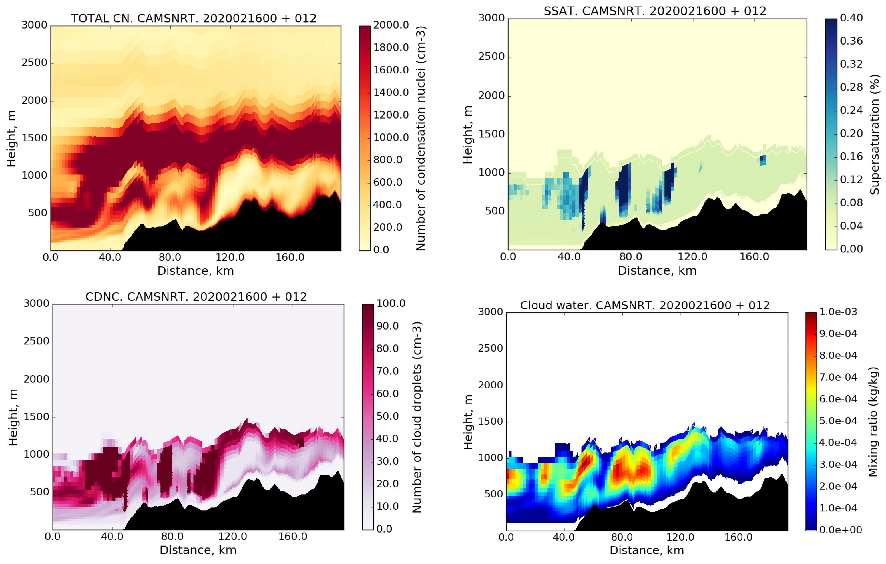
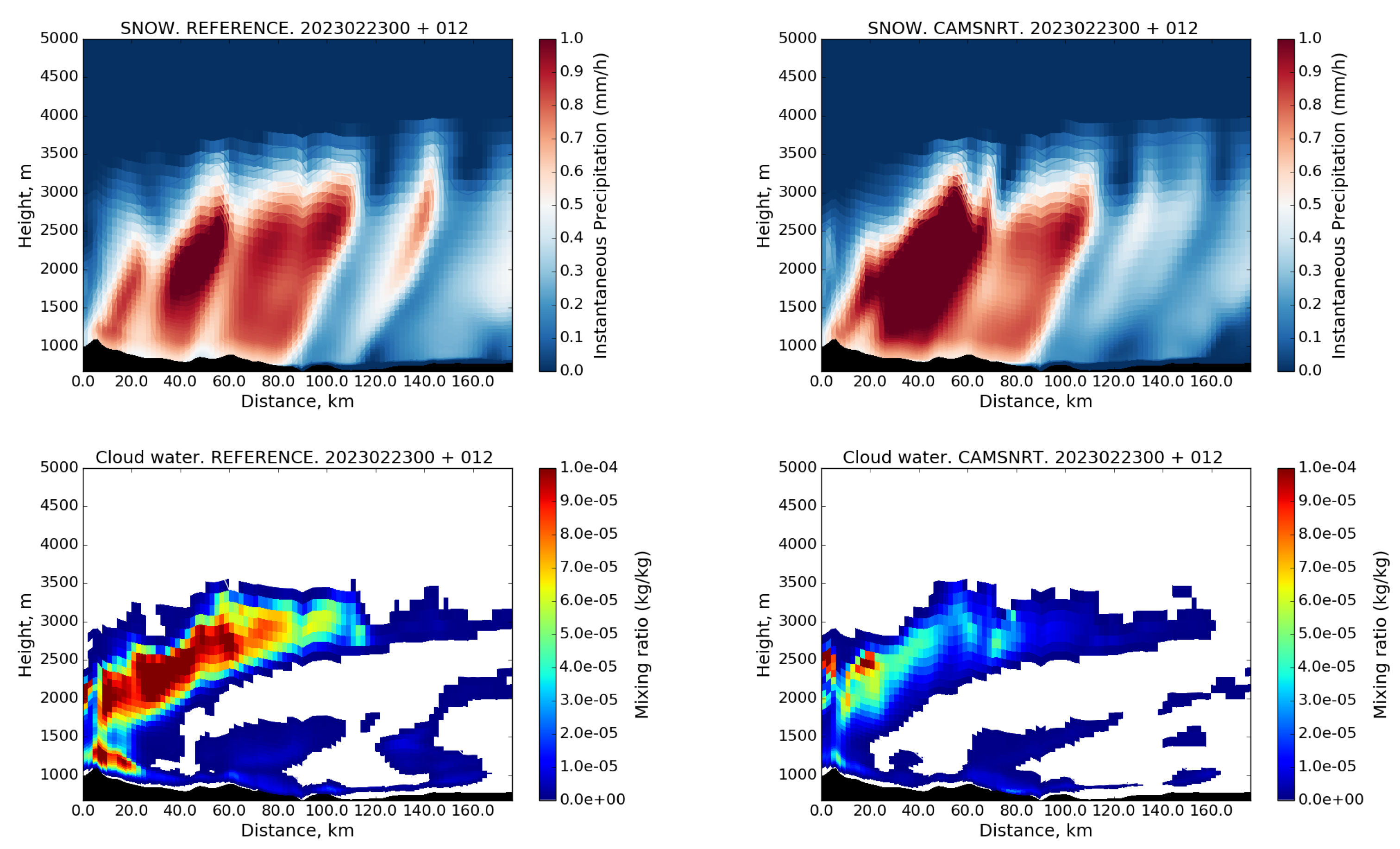
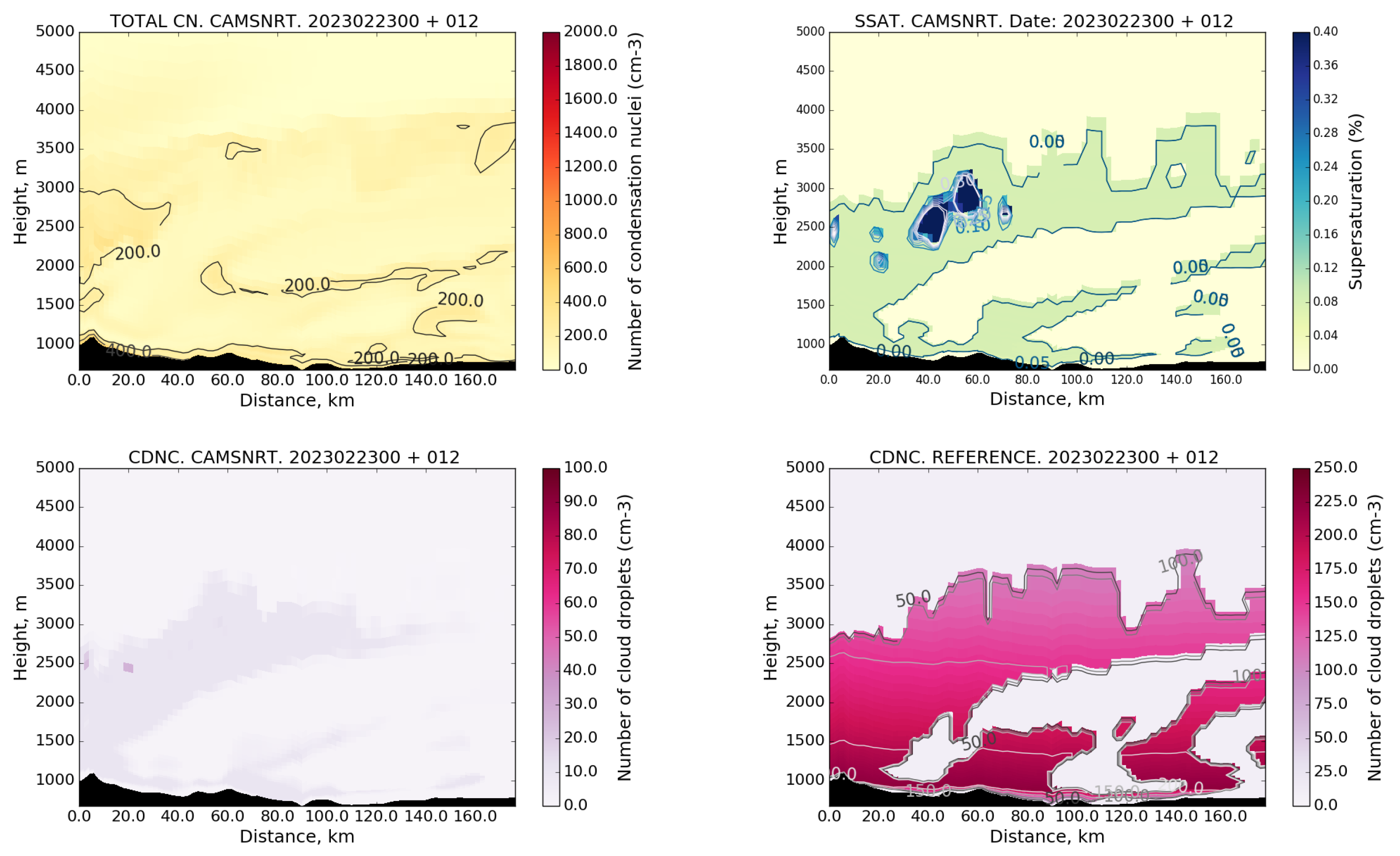
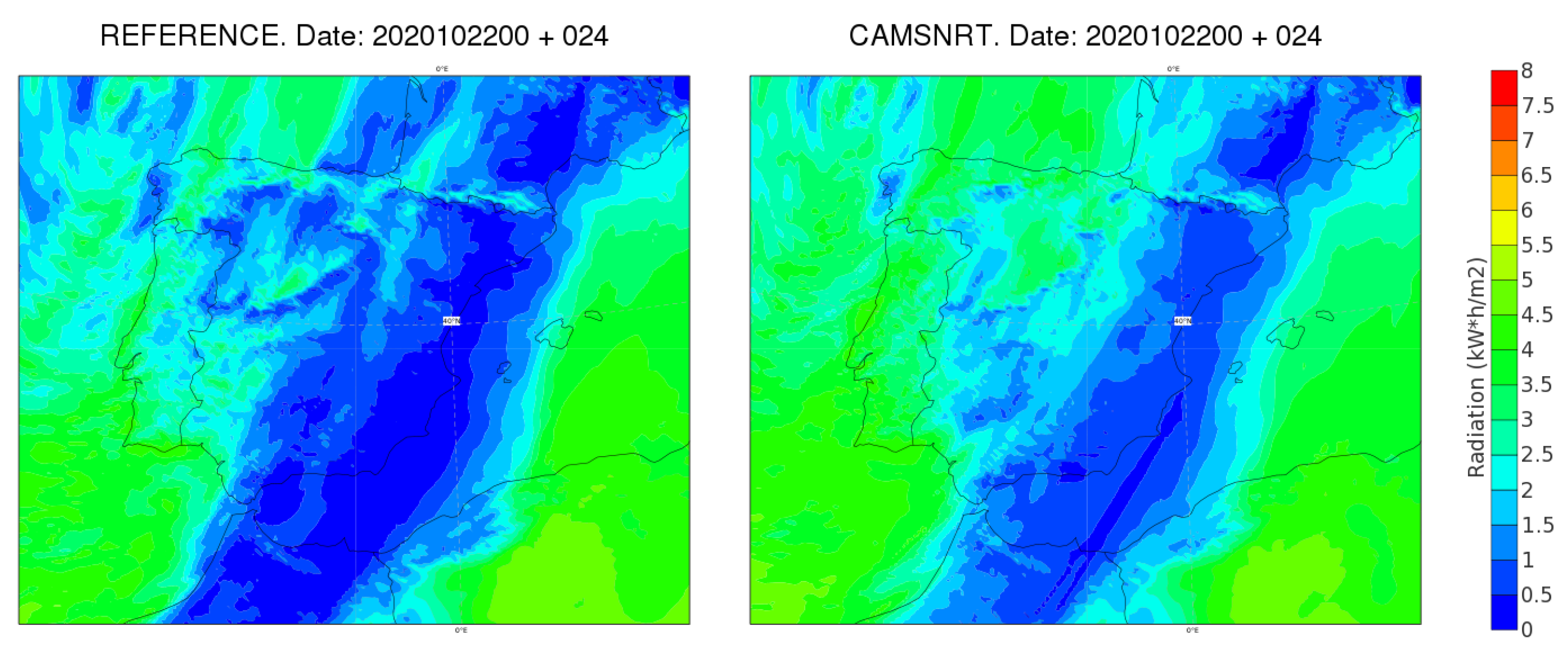
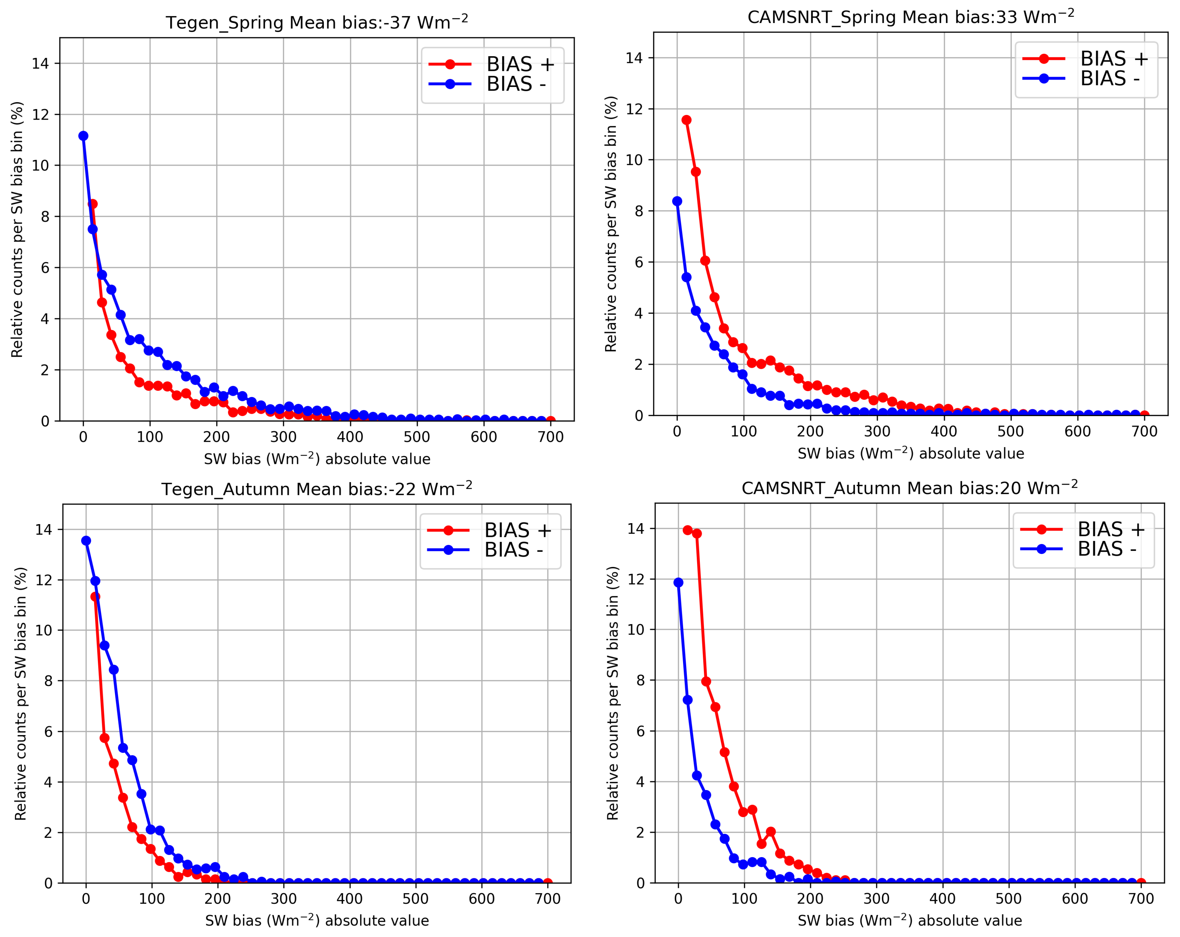
Table 1.
Aerosol species, bin size limits, and parameters for size distribution are the same as in IFS-AER (Table 1 in [9]). The bin limits are the maximum radius () and minimum radius () of a particle to be included in the bin, is the “number mode radius” of the log-normal size distribution, is the geometric standard deviation, is a correction factor applied for the calculation of the PNC of each aerosol type, is the hygroscopic parameter obtained from [19], and is the mass extinction in m2 kg−1 at relative humidity.
| Aerosol Species | Bin Limits (μm) | ||||||
|---|---|---|---|---|---|---|---|
| Sea salt 1 (film drop mode) | 0.03–0.5 | 2160 | 0.1992 | 1.9 | 0.318 | 1.28 | 4048.34 |
| Sea salt 2 (jet drop mode) | 0.5–5.0 | 2160 | 1.992 | 2.0 | 0.255 | 1.28 | 432.98 |
| Sea salt 3 (spume drop mode) | 5.0–20 | 2160 | 1.992 | 2.0 | 7.284 | 1.28 | 122.77 |
| Desert dust 1 (fine dust bin) | 0.03–0.55 | 2610 | 0.29 | 2.0 | 0.151 | 0.0 | 2496.68 |
| Desert dust 2 (coarse dust bin) | 0.55–0.9 | 2610 | 0.29 | 2.0 | 1.610 | 0.0 | 955.08 |
| Desert dust 3 (super-coarse dust bin) | 0.9–20 | 2610 | 0.29 | 2.0 | 13.140 | 0.0 | 406.53 |
| Hydrophobic organic matter | 0.05–20 | 2000 | 0.021 | 2.24 | 0.894 | 0.0 | 2321.03 |
| Hydrophilic organic matter | 0.05–20 | 2000 | 0.021 | 2.24 | 0.894 | 0.3 | 3481.84 |
| Hydrophobic black carbon | 0.005–0.5 | 1000 | 0.0118 | 2.0 | 1.119 | 0.0 | 13,487.80 |
| Hydrophilic black carbon | 0.005–0.5 | 1000 | 0.0118 | 2.0 | 1.119 | 0.1 | 13,487.80 |
| Sulfates | 0.005–20 | 1760 | 0.0355 | 2.0 | 1.002 | 0.6 | 6296.94 |
| Nitrate fine mode | 0.005–0.9 | 1730 | 0.0355 | 2.0 | 0.997 | 0.64 | 7361.85 |
| Nitrate coarse mode | 0.9–20 | 1400 | 1.992 | 2.0 | 1.022 | 0.9 | 7425.71 |
| Ammonium | 0.005–20 | 1760 | 0.0355 | 2.0 | 1.002 | 0.6 | 483.48 |
Table 2.
Aerosol properties for deposition. Fraction of aerosols included in droplets.
| Aerosol Species | |
|---|---|
| Sea salt 1 (film drop mode) | 0.9 |
| Sea salt 2 (jet drop mode) | 0.9 |
| Sea salt 3 (spume drop mode) | 0.9 |
| Desert dust 1 | 0.7 |
| Desert dust 2 | 0.7 |
| Desert dust 3 | 0.7 |
| Hydrophobic organic matter | 0.0 |
| Hydrophilic organic matter | 0.7 |
| Hydrophobic black carbon | 0.0 |
| Hydrophilic black carbon | 0.7 |
| Sulfates | 0.7 |
| Nitrate fine mode | 0.4 |
| Nitrate coarse mode | 0.4 |
| Ammonium | 0.4 |
Table 3.
Point verification results for the two periods referred to in the text. Bias and standard deviation (STDV) for surface pressure, wind speed, 2 m temperature, relative humidity, cloud cover, and 24 h accumulated precipitation.
Table 3.
Point verification results for the two periods referred to in the text. Bias and standard deviation (STDV) for surface pressure, wind speed, 2 m temperature, relative humidity, cloud cover, and 24 h accumulated precipitation.
| REFERENCE | CAMSNRT | |||
|---|---|---|---|---|
| AUTUMN | BIAS | STDV | BIAS | STDV |
| Surface Pressure | 0.15 | 0.81 | 0.04 | 0.80 |
| Wind Speed | 0.69 | 1.48 | 0.71 | 1.47 |
| 2 m Temperature | −0.34 | 1.46 | −0.21 | 1.43 |
| Relative Humidity | −0.55 | 10.64 | −1.36 | 10.68 |
| Cloud Cover | 0.32 | 2.72 | 0.23 | 2.75 |
| 24 h Accumulated Precipitation | −0.27 | 8.68 | −0.05 | 8.57 |
| SPRING | BIAS | STDV | BIAS | STDV |
| Surface Pressure | −0.05 | 0.90 | −0.10 | 0.88 |
| Wind Speed | 0.65 | 1.49 | 0.69 | 1.49 |
| 2 m Temperature | −0.03 | 1.56 | 0.10 | 1.54 |
| Relative Humidity | −4.14 | 11.39 | −4.44 | 11.27 |
| Cloud Cover | 0.23 | 2.83 | 0.21 | 2.84 |
| 24 h Accumulated Precipitation | −1.08 | 6.14 | −0.62 | 5.76 |
Disclaimer/Publisher’s Note: The statements, opinions and data contained in all publications are solely those of the individual author(s) and contributor(s) and not of MDPI and/or the editor(s). MDPI and/or the editor(s) disclaim responsibility for any injury to people or property resulting from any ideas, methods, instructions or products referred to in the content. |
© 2024 by the authors. Licensee MDPI, Basel, Switzerland. This article is an open access article distributed under the terms and conditions of the Creative Commons Attribution (CC BY) license (https://creativecommons.org/licenses/by/4.0/).
Share and Cite
MDPI and ACS Style
Martín Pérez, D.; Gleeson, E.; Maalampi, P.; Rontu, L. Use of CAMS near Real-Time Aerosols in the HARMONIE-AROME NWP Model. Meteorology 2024, 3, 161-190. https://0-doi-org.brum.beds.ac.uk/10.3390/meteorology3020008
AMA Style
Martín Pérez D, Gleeson E, Maalampi P, Rontu L. Use of CAMS near Real-Time Aerosols in the HARMONIE-AROME NWP Model. Meteorology. 2024; 3(2):161-190. https://0-doi-org.brum.beds.ac.uk/10.3390/meteorology3020008
Chicago/Turabian StyleMartín Pérez, Daniel, Emily Gleeson, Panu Maalampi, and Laura Rontu. 2024. "Use of CAMS near Real-Time Aerosols in the HARMONIE-AROME NWP Model" Meteorology 3, no. 2: 161-190. https://0-doi-org.brum.beds.ac.uk/10.3390/meteorology3020008