
Computational Fluid Dynamics Methodology to Estimate the Drag Coefficient of Balls in Rolling Element Bearings

1
LabECAM, ECAM LaSalle Campus de Lyon, Université de Lyon, 69321 Lyon, France
2
INSA Lyon, CNRS, LaMCoS, UMR5259, 69621 Villeurbanne, France
*
Author to whom correspondence should be addressed.
Dynamics 2024, 4(2), 303-321; https://0-doi-org.brum.beds.ac.uk/10.3390/dynamics4020018
Submission received: 6 March 2024
/
Revised: 8 April 2024
/
Accepted: 12 April 2024
/
Published: 25 April 2024
Abstract
:The emergence of electric vehicles has brought new issues such as the problem of rolling element bearings (REBs) operating at high speeds. Losses due to these components in mechanical transmissions are a key issue and must therefore be taken into account right from the design stage of these systems. Among these losses, the one induced by the motion of rolling elements, known as drag loss, becomes predominant in high-speed REBs. Although an experimental approach is still possible, it is difficult to isolate this loss in order to study it properly. A numerical approach based on CFD is therefore a possible way forward, even if other issues arise. The aim of this article is to study the ability of such an approach to correctly estimate the drag coefficient associated with the motion of rolling elements. The influence of the numerical domain extension, the mesh refinement, the simplification of the ring shape, and the presence of the cage on the values of the drag coefficient is presented. While it seems possible to compromise on the calculation domain and mesh size, it appears that the other parameters must be taken into account as much as possible to obtain realistic results.
1. Introduction
The decarbonisation of the road transport is a shared objective for the automakers all around the world in order to protect the environment [1]. The automotive industry aims to become in this senses carbon neutral in 2050 and zero-emission vehicles are being developed to this end using batteries or fuel cell technology. However, the emergence of electric vehicles has brought new issues to the fore, such as the problem of rolling element bearings (REBs) operating at high speeds. Losses due to these components in mechanical transmissions are a key issue [2] and must therefore be taken into account right from the design stage of these systems. It is indeed possible to evaluate the power loss dissipation using the empirical power loss model proposed by Harris [3] or using the global model developed by SKF Company [4] recently detailed in part by Morales and Wemekamp [5]. However Harris model does not provide accurate results in high-speed REB [6]. The drag loss induced by the motion of the rolling elements of the REB must be modelled and then combined with the latter in order to adjust the power loss value. When using SKF model, the estimated power loss greatly overestimates measurements [7,8], and it seems preferable sometimes not to use the drag power loss component proposed by the model and to replace it by a traditional term as proposed by Harris [3]. As an alternative to these models, experimental approaches have been employed previously by Macks et al. [9], Zaretsky et al. [10], Schuller et al. [11], and recently by Niel et al. [6] and Yan et al. [12]. In this approach it is difficult, if not impossible, to isolate the drag loss in order to study it properly. However, among the losses in high-speed REB, the drag loss can become predominant when shaft speed increases. In the past, the drag force had to be estimated for its contribution to the balance of forces applied to the rolling elements in a quasi-static approach as Rumbarger et al. in ball bearings [13] or Nelias et al. in cylinder bearings [14]. A numerical approach based on computational fluid dynamics (CFD) is therefore a possible way forward and has been widely used for mechanical transmission as presented by Concli in his comprehensive review of the available CFD approaches [15]. Among many other studies Hill et al. [16] has simulated the windage power losses for isolated rotating spur gear and Fondelli et al. [17] when the gear is in a confined space. Concli et al. [18] employed the volume of fluid method [19] for the analysis of power losses in a planetary speed reducer, and Hildebrand et al. [20] employed the same method for investigating the influence of gearbox housing geometry and oil guide plates on churning power losses. Recently Concli and Mastrone [21] have optimized numerically the lubrication of an entire system including shafts, gears and bearings with all the rolling elements. In specifically considering bearings this time, Hu et al. [22] and Wu et al. [23] simulated the oil volume fraction in the complete ball bearing in order to investigate the temperature distribution inside the bearing. Liebrecht et al. [24] used the same method for estimating the drag and churning losses on tapered roller bearings this time. Other studies have used CFD method for studying the lubricant flow distribution in the bearing: Adeniyi et al. investigated, for example, the oil jet break when the lubricant is introduced in the bearing chamber via the inner race region of the bearing into the rolling elements interstices [25]. For that, one ball located in periodic portion of the entire cavity is employed. Peterson et al. [26,27] employed three consecutive balls this time associated with periodic conditions; Aria et al. [28] employed the complete ball bearing for the simulation of the lubricant flow in the bearing. Few investigations have been conducted to estimate the drag losses, such as Feldermann et al. [29] or Wang et al. [8]. Drag forces involve the use of a drag coefficient whose value was initially taken as that observed for an isolated sphere. Marchesse et al. [30] contradicted this latter point and highlighted the role of the relative spacing of the balls on the drag coefficient value using CFD method based on three balls accompanied with periodic boundary conditions. Later, the same approach was used to highlight the importance of the oil volume fraction in the estimation of the drag power losses in cylinder roller bearing [7]. A numerical approach can be therefore very useful, as long as it is not too time-consuming while offering consistent drag coefficient values, since it is not possible to validate directly their value. Therefore, this raises a number of questions, for example, the number of balls that should be present in the computation, the mesh quality (i.e., the number of elements layers) in the contact region between the ball and the race, the ring shape, etc. Some investigations address these issues. Feldermann et al. [29] simulated, for example, the flow in the entire bearing and the computed flow field is thereafter mapped to a less expensive single bearing chamber model. Marchesse et al. [30] have, for example, investigated the influence of the mesh refinement on the drag coefficient when studying angular contact ball bearing but in a very simplified environment (without any rings or cage). Some authors have used a different number of layers in the contact region: three elements in Adeniyi et al. [25], and six elements in Arya et al. [28] investigations. It can be noticed that there is therefore no consensus on which numerical method to use and which numerical parameters are important to stipulate, the others being of less importance in the approach. For that, the present article aims at investigating numerically the drag coefficient of balls inside a radially loaded low-load deep groove ball bearing (DGBB). This work participates to a wider study to investigate load-independent power losses for which the drag coefficient is to be evaluated [31].
This paper is organized as follows. First, the bearing specification, the oil lubrication and the rotational speed are reported. The numerical approach is then introduced followed by some results which provide information about the mesh influence and the minimum number of balls that should be present in the numerical domain. Finally, this approach is used for studying the influence of both geometrical and dynamics parameters, and also the cage type and its thickness on the drag coefficient value.
2. Bearing Specification
As deep groove ball bearings (DGBBs) are often used on a high-speed shaft gear unit for automotive application, the design parameters of the following deep groove ball bearing (DGBB) tested here are provided in Table 1. There are eight balls so that the angular periodicity inside the chamber equals to 45°. The cage is a stamped metal cage like. Its thickness and its cross-sectional area perpendicular to flow modified by the cage thickness, mm and m², respectively. The gap between two consecutive balls equals , which does not allow the wake to develop perfectly. Therefore, the drag coefficient value will be less than the value observed when one single isolated sphere is considered [30]. Moreover, the bearing has no seal so that the lubricant has the possibility to flow in and out.
3. Rotational Speed
One considers here the radially loaded DGBB, i.e., and ( and being the radial and the axial load, respectively), and hence, the radial equivalent load reads [32]. During the experiments associated with this investigation, the radial equivalent load equals one sixth the static capacity (), leading to at minimum. The sliding effect is then negligeable in comparison to the rolling effect. A pure rolling hypothesis then seems reasonable, and one can thus consider the tangential velocities of all the balls and the tangential velocity of the rings as coinciding. Consequently, no distinction is made between the balls in the loaded region and the unloaded region, discarding the physical phenomenon in the contact region.
The rotational speed of the DGBB is fixed to 9000 rpm so that , which is sufficiently high so that drag force participates significantly to the power losses. The cage and the rolling element rotation speeds equal rpm and rpm, where . It will be seen later that relative speeds according to the cage must be evaluated because the numerical computations are made in the cage reference frame.
If the cage velocity is employed in the Reynolds number, then , a sufficiently high value for the effects of turbulence to be strongly present.
4. Oil Lubrication
The numerical simulations are performed with a gearbox mineral oil, the physical properties of which are given in Table 2. Since the present study does not investigate the physical phenomenon occurring in the contact region, only the temperature dependence of both the density and the dynamic viscosity is considered here. Most of the simulation is performed at 50 °C leading to the following oil physical properties: kg/m3; cSt. When the lubrication is based on an oil bath, the oil level is generally chosen as half the diameter of the lowest rolling element. Therefore, the ratio between the volume occupied by the oil in the bearing and the total volume inside the bearing, namely the oil volume fraction (, nearly equals 7%. When the bearing is in motion, the oil in the bearing is then totally dispersed in an air–oil mist and can be considered as a homogenous fluid in a first approximation. The effective properties of the mixture can be evaluated from the two formulations for the effective density and the effective dynamic viscosity [33], respectively:
with the air properties evaluated at 50 °C, i.e., = 1.092 kg/m3 and = Pa.s and being the oil mass fraction. The effective properties reads kg/m3 and Pa.s. These two values will be used in the computation based on a homogeneous fluid inside the bearing.
5. Numerical Approach
The numerical approach that is used here is highly simplified for three main reasons: (1) one wants to see the capacity of such simplified approach to correctly estimate the flow inside the bearing for the estimation of the drag coefficient, (2) some information is difficult to estimate and deals with the contact region, which is not the purpose of our study, and (3) the simulation of this kind of complex flow exceeds the current capabilities of computer codes. The simplifications will be set out gradually in the text.
As mentioned in the previous section, the bearing cavity is supposed to be full of a homogeneous mixture of air and oil. This mixture never really exists in the cavity, but in some operational configurations, this is roughly the case. This can happen in a high-speed configuration, for example, when inner ring jet lubrication is employed as discussed by Parker and Signer during their experiments [34]. Thanks to this hypothesis, they proposed a formulation for estimating the oil volume fraction in the bearing cavity. If the mixture is supposed to be homogeneous in the cavity, that means each ball has the same fluid environment. As a result, the full problem features multiple identical regions, i.e., periodicity (Figure 1). The numerical approach used here considers then only a fraction of the entire REB associated with periodic boundary conditions. A few years ago, the authors investigated the influence of relative distance between balls on the drag coefficient and showed that the periodic conditions allowed a ball to be correctly influenced by its upstream and downstream balls [30]. However, while this approach has been afterward successfully used to study flow within the bearing [26,27], it has never been used to estimate the drag coefficient when considering the environment of the balls, i.e., the rings, the cage and their velocities in the REB. Many questions arise then as to, for example, the minimum number of balls to be included, or the minimum number of mesh layers in the contact region in the simulation in order to have no more impact on the drag coefficient value.
5.1. Numerical Domain
The numerical domain considering one ball among the eight balls is proposed in Figure 2. When the computation considers few balls, the numerical domain is built by multiplying the former domain in order to obtain one single numerical domain. The diameter of the ball that is simulated equals 21 mm as it is for the real REB ball. However, for the reason of continuity of the mesh in the contact region, the inner race radius is shortened and the outer race radius is increased so that the gap value equals 52.5 μm (i.e., ). This numerical value is of the same order of magnitude as the 95 μm gap employed by Adeniyi [25] and both the 161 μm and 74 μm gaps for the DGBB and radial needle roller bearing, respectively, in investigations by Peterson [26,27]. The axial extension of the domain equals 3.5 times the DGBB width (i.e., nearly 100 mm) in the two axial directions, while the outer radius and the inner radius of domain equal the outer DGBB radius (i.e., 60 mm) and 0.9 times the bore radius (i.e., 25 mm). Both the axial and the radial extensions of the domain outside the bearing are then sufficiently high so that the flow in this region does not greatly influence what happens inside the bearing. It can be noticed that the numerical domain represents the bearing cavity at rest. The skewing of some elements (the shoulder, for example) when the bearing rotates could deform it, which is not the purpose of the present study.
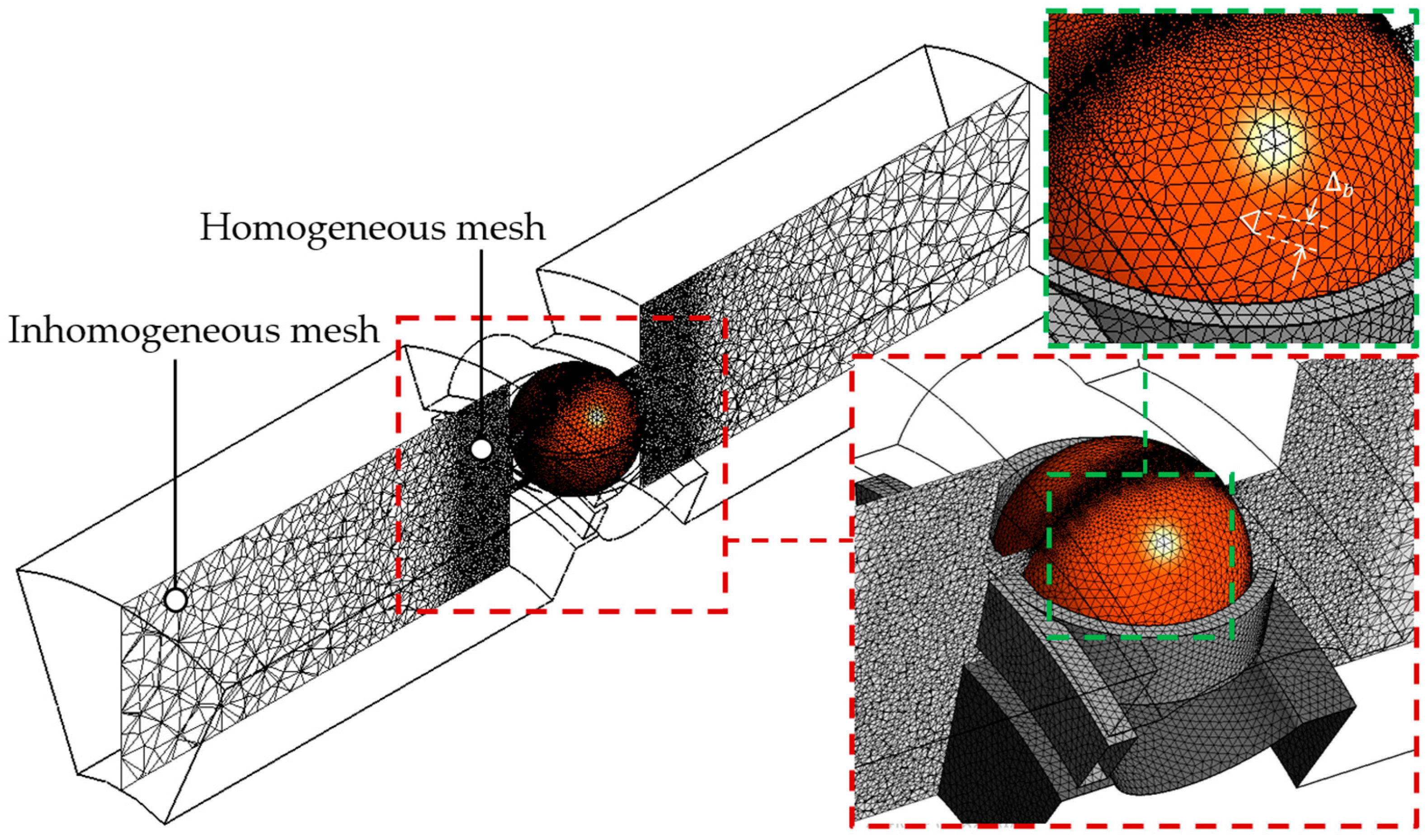
5.2. Mesh
The influence of the mesh will be investigated later in the article. The equations are solved on an inhomogeneous tetrahedral mesh with a strong clustering close to the balls to capture the near-wall turbulent region (Figure 2). A structured mesh is built near the balls wall with the height of the first cell (i.e., prism shape) chosen so that the dimensionless wall parameter is less than 2, which is in good agreement with the turbulence model used here. The structured mesh is composed with an inflation of prism layers constructed with an expansion equal to 1.05 along 10 layers where it is possible. This number of layers is not possible in the contact region due to the small gap, where generally five layers are built and represent nearly half of the gap distance. The maximum value of the edge size of the first cells on the balls, (Figure 2) will vary later in order to see its influence on the drag coefficient value. In previous investigations, the authors showed that using an edge size equal at maximum to is sufficient to reach a correct drag coefficient [30]. Beyond this first structured mesh, a homogeneous unstructured mesh with a mesh size of is built inside the bearing and to a certain axial extension outside the bearing. Finally, beyond to this mesh, the mesh size on the outside of the bearing increases with an expansion factor equal to 1.3 (Figure 2).
5.3. Boundary Conditions
The boundary conditions are summarized in Figure 3. No slip wall conditions are imposed in the inner and the outer rings, the cage and the balls surfaces. Since the computation is made in the cage reference frame, , relative velocity must be evaluated, so that the inner and the outer rings angular speeds equal rpm and rpm, respectively. The angular speed of the ball relative to the cage reference frame equals rpm. The index r recalls that the angular speeds are evaluated in the cage reference frame. The inner and outer rings rotate according to the absolute z axis, while the balls rotate around their own axis. The four surfaces that have their unit normal vector aligned with the y axis let the flow move into or out of these surfaces (opening boundary condition). The symmetry condition, i.e., null normal velocity component, is imposed to the two surfaces that have their unit normal vector aligned with z axis. The two surfaces that have their unit normal surface aligned with tangential direction represent periodicity condition. This means that the flow entering the computational model through one periodic plane is identical to the flow exiting the domain through the opposite periodic plane.
5.4. Governing Equations
The Navier–Stokes equations are solved for incompressible airflow. Numerical local solutions are obtained using the commercial software ANSYS-CFX 2022 R2 based on the Reynolds-averaged Navier–Stokes theory [35]. The finite volume discretization method approximates the differential equations by a system of algebraic equations for the variables at some set of discrete locations in space. The state equations are solved with respect to a rotating reference frame associated with the cage for unsteady state flows with Coriolis and centrifugal effects being taken into account. The low-Reynolds SST k-ω turbulent model [36] is used to close the time-averaged continuity and momentum equations for an incompressible viscous flow without body force.
5.5. Time Discretization
Transient computations are performed in the present study, and the time step () is chosen so that the dimensionless time step () satisfies . It can be noticed that this value is twice the value used in reference [30], but one observes that the drag coefficient value is less sensitive when balls are confined in its environment rather than in an infinite medium. For example, if the timestep is divided by 2, the drag force varies less than 1%.
5.6. Convergence Criteria
Convergence is achieved here without any problem since the normalized residuals of the equations reached a value below and the aerodynamic components of the balls behave nearly periodically in accordance with structure detachments. When few balls are simulated, all the force intensities are similar for all of them (2.9% relative difference with mean-averaged value at maximum), which highlights that the use of the periodic conditions is satisfying.
6. Setting up the Numerical Approach
6.1. Time Evolution of the Drag Coefficient, Streamlines and Pressure Distribution
The parameter of most interest in this study is the drag coefficient:
where is the drag force exerted by the fluid on the ball, is the air–oil mist density, is the cage velocity and A is the cross-sectional area introduced previously in bearing specification section. The drag coefficient predicted numerically is plotted during the computation (Figure 4), and the latter is stopped when the convergence is met (on time equal to 0.45 in Figure 4). The averaging interval for the estimation of the drag coefficient is taken sufficiently large compared to the typical time scale of the fluctuations. Numerical results given in Figure 5 are obtained regardless of the numerical configuration studied later in the article. Streamlines and complex circulations of the fluid are noticed in the bearing cavity due to all the moving parts (i.e., the rolling elements, the cage and the rings), which is in accordance with what one expects due to the moving parts and also with Peterson et al.’s observations [26]. The fluid velocity decreases near the gap leading to an increase in the pressure coefficient, , where is the pressure at a location far from the REB cavity (i.e., symmetry surface in Figure 3). The inhomogeneous pressure distribution is thereafter the cause of the drag force.
6.2. Influence of the Mesh
It is always desirable to use a mesh based on a minimum number of nodes or cells without compromising the quality of the numerical prediction in order to reduce the computational time. Here, the influence of both the number of the cells in the gap between the ball and the ring, and the cell size on the ball, , on the drag force value is investigated. For the first study, five different meshes are used based on different numbers of element in the gap between the rings and the ball, while the edge size of the first cells on the ball equals as proposed previously by the author for one isolated ball [30]. This test has been performed with one ball, as in the example of Figure 3. The coarsest mesh comprises only one element in the gap, while the finest one comprises five layers. No structured mesh has been built in the ball in this test leading to a dimensionless wall parameter . The finest mesh has 100 more cells that the coarsest (Table 3). One notices that using one single element in the gap leads to a drag coefficient value less than 24% below the value obtained when five layers have been used (Table 3). Moreover, when the mesh comprises three layers, as was the case in Adeniyi et al.’s investigation [25], the drag coefficient value nearly equals 5%, the value reached using the finest mesh in the gap. It is a very interesting consensus since the number of the element in the finest mesh is three times the number of the mesh when three layers are present. However, employing a structured mesh is sometimes preferable when one wants to manage the height of the first cell so that becomes less than 5 depending on the type of turbulent model employed. If one does so, then the first height nearly equals 20 μm (), leading to more than five layers in the gap (i.e., the structured mesh followed by the unstructured mesh). The consequence is a 5% difference on the drag coefficient values in comparison with the simplified case based on only three layers and without any structured mesh in the gap between the ring and the ball.
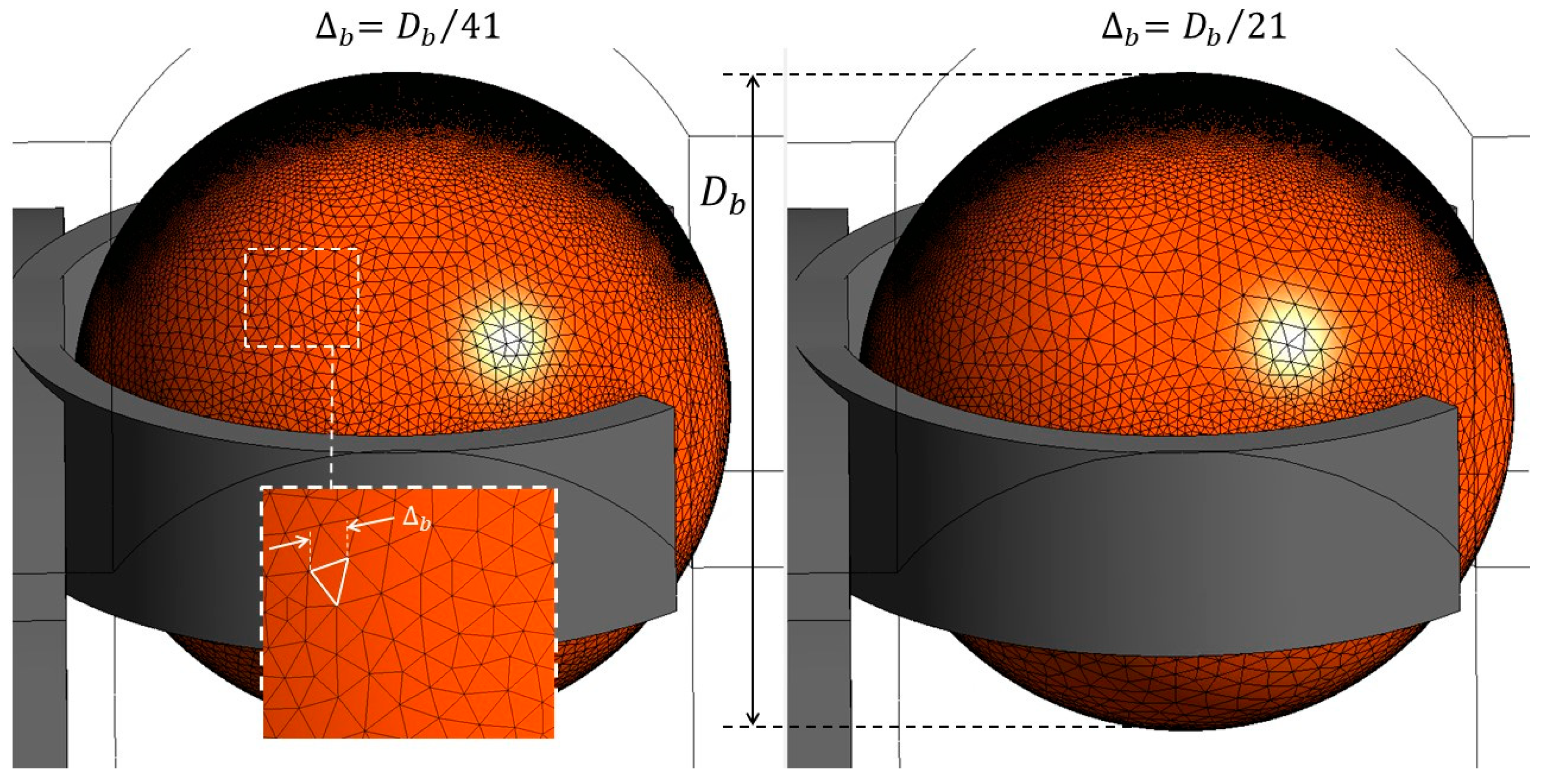
A previous investigation by the authors [30] used a mesh based on edge size of the first cells equal to when considering only balls without any moving solids in their vicinity (i.e., rings or cage). It remains to be seen if this refinement is sufficient when the two rings and the cage are present this time in the computation. For that, three meshes are built using three elements in the gap between the ball and the rings and based on different values for the edge size of the first cell on the ball (see Figure 6 with and ). It should be noted, however, that not all the cells located on the ball are of this size because the size of the cells located near the gap between the ball and the ring is shorter. The reason for this is to respect the good quality of the mesh. Consequently, the cells that do not have the same size are located in a region between the gap and the cage (see Figure 6), so this only concerns a limited number of cells. However, one notices that a 9% relative difference is observed between the drag coefficients predicted from the meshes with and , respectively (Table 4). This relative difference is less when (relative difference equals 2%). Once again, this highlights the sensitivity of the solution to the mesh size and using a mesh so that the size of the cells on the ball equal to is satisfying, as was the case when no moving walls were around the balls. In the following parts of the article, three elements in the gap and cells on the balls that have size equal to will be employed for the meshes.
6.3. Influence of the Number of Balls
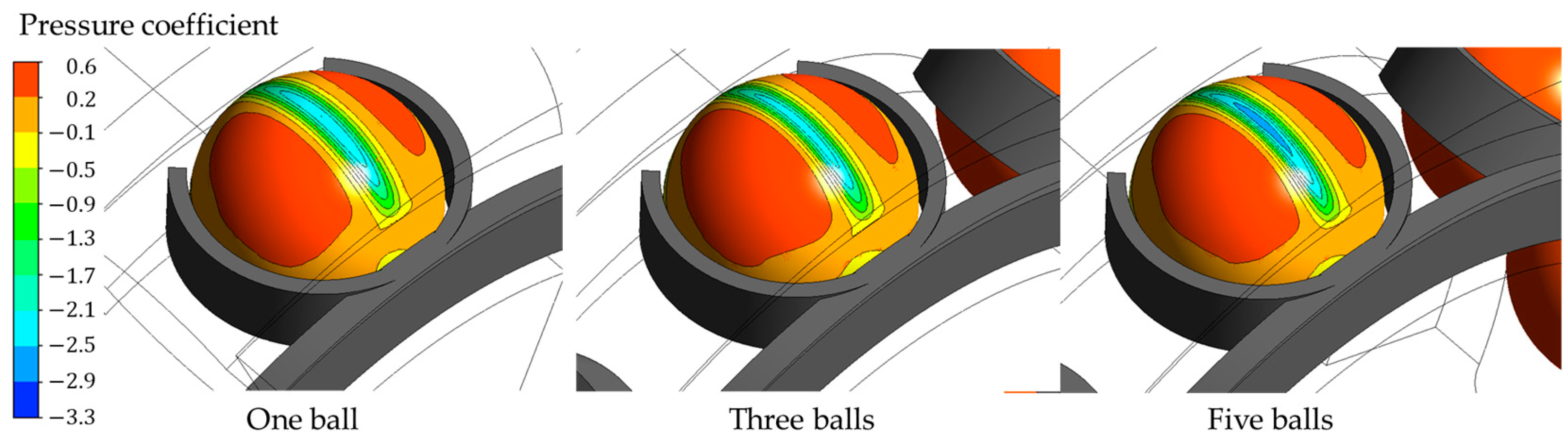
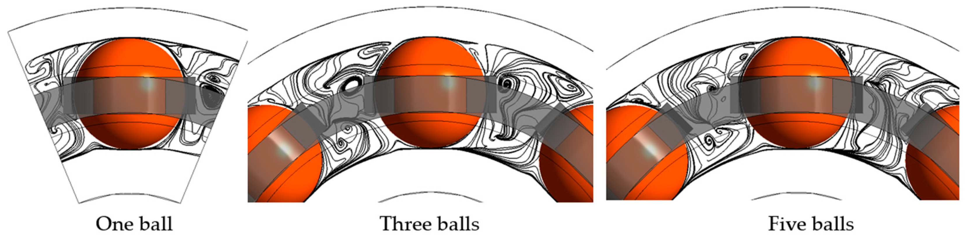
To reduce the computation time, it is possible to reduce the number of balls simulated in the numerical domain since, as mentioned previously, the air–oil mixture is supposed to be homogeneous (Figure 1), and thus, there are several identical regions. Using one or more balls in the computation should then induce the same drag coefficient value. In order to evaluate this possibility, it was decided to put a ball in front of and a ball behind the ball whose drag coefficient is to be estimated when more than one ball is studied. Three configurations are therefore investigated, i.e., numerical domains comprising one, three or five balls (Figure 7). No structured mesh has been used during this test, three elements are present in the gap and the edge size of the first cells on the balls equal It can be seen that using three or five balls induces nearly identical drag coefficient values since only 1% relative difference is noticed between the two configurations (Table 5). One significant difference arises when one ball is used rather than five balls in the numerical domain, since the difference increases to 11%. These subtle differences are confirmed when observing the distribution of the pressure coefficient and the streamlines for the three cases that do not vary significantly (Figure 8 and Figure 9).
6.4. Importance of the REB Environment in the Computation
As mentioned previously, the authors investigated three stationary and aligned balls associated with periodic conditions without considering the presence of the two rings and the cage [30]. The purpose was solely to investigate at that time the influence of the distance between two consecutive balls () on the drag coefficient. Since one wants to reach here a very simplified numerical approach, one wonders if considering the rings, the cage and their rotations is important in the numerical approach. For that, the method reached in the previous sections is used on a bearing satisfying in order to compare the drag coefficient value with the configuration in reference [30]. The drag coefficient value when the REB is considered is nearly two times the one when only three aligned and stationary balls are considered (Table 6). This is mainly due to the rotation of the balls that maintain a high value of the pressure coefficient in the region near the contact, which is not the case when three balls without the REB environment is investigated. Since the latter configuration is highly simplified, it should not reproduce the flow in the bearing, and therefore, the drag coefficient value is not well estimated.
Following the same idea of simplifying the numerical domain, the value of osculation () which represents the ratio between the raceway radius and the RE diameter is rarely given by manufacturers. Rather than building a numerical domain satisfying [3], which seems to be a common value, flat raceways both for the inner and the outer rings have been built () with . This could also avoid the problem for the mesh in the gap between the ball and the raceway by limiting the size of this region. One observes than this high simplification leads to a great modification of the drag coefficient value since its sign becomes negative and its absolute value is reduced (Table 7). This means that while the ball moves forward, it is also driven in this direction by a force exerted by the fluid. Since non-infinite osculation (i.e., flat raceways) is always considered, the ring shape cannot be simplified to such an extent, and osculation should be considered in the numerical approach.
6.5. Conclusion on the Study of the Numerical Approach
The previous sections have enabled us to define a numerical approach based on the following points:
- At least three balls should be simulated in the numerical domain associated with periodic boundary conditions in the two lateral surfaces;
- The rings and their shape, the cage and their rotations should be imposed;
- Three elements should be present at minimum in the gap between the ring and the rolling element;
- The size of the first cells on the balls () should satisfy the criteria where is the ball diameter.
The rest of the study will use this approach to study the influence of some parameters such as the relative spacing of the balls, the type of the cage and its thickness on the numerical value of the drag coefficient. The aim of the study is to assess the impact of the various parameters on this coefficient and not to give a general formulae for it.
7. Influence of Geometrical and Dynamics Parameters
Based on what has been shown above, a numerical approach, which is able to take into account the interior geometry of the REB and the kinematics of the rings and the rolling elements, has been defined. It could be interesting thus to analyse if the modification of the geometric parameters induces a modification of the value of the drag coefficient or if the numerical approach is not sensitive enough.
7.1. Influence of the Distance between Two Consecutive Balls
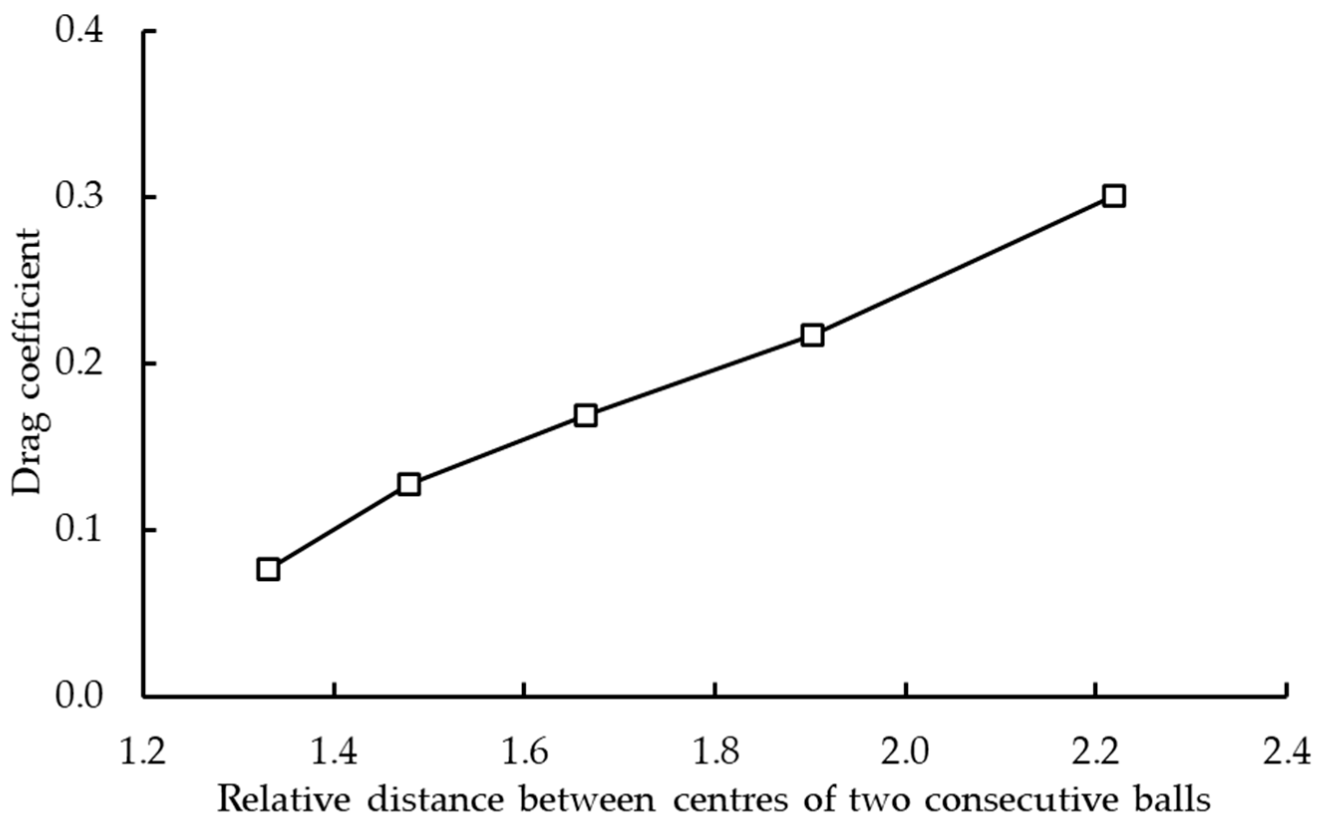
Previous investigations highlighted the influence of the relative distance between two consecutive balls on the drag coefficient [30]. It has been demonstrated that increasing the relative distance leads to a linear increase in the drag coefficient when the relative distance remains lower than three times the ball diameter. However, this investigation considered isolated aligned spheres, which is not the case in REB. Five simulations are thus carried out here with different relative distances in the REB environment: corresponding to the number of balls, 10, 9, 8, 7 and 6, respectively, in the bearing (Figure 10).
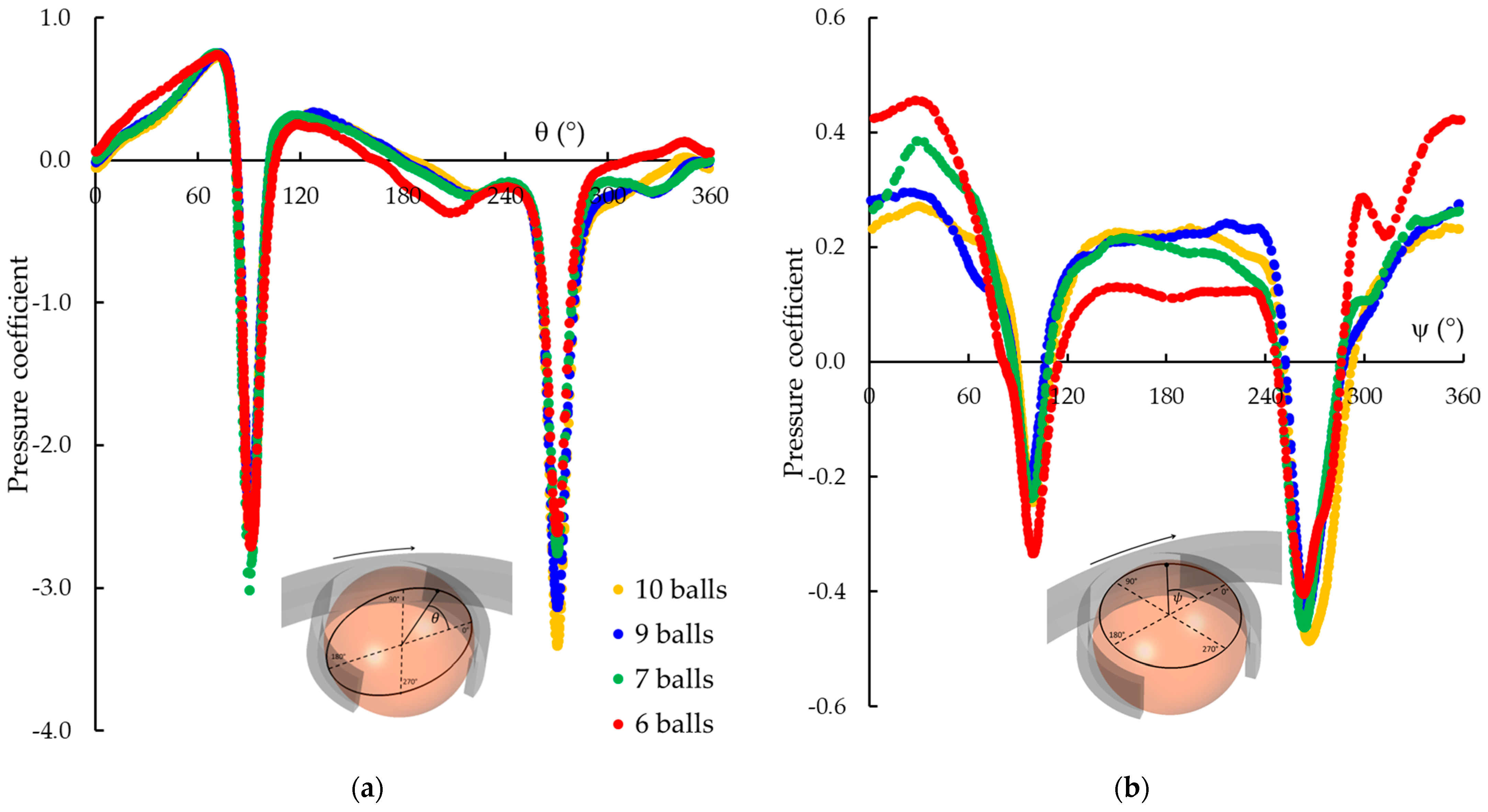
One observes that the relative distance has an influence on the pressure coefficient on the ball (Figure 11) since the size of the region where the high pressure occurs (region A in Figure 11) increases towards the front of the balls. The pressure then acts in a region where the unit vector is more aligned with the flow, and as a result, its action is increasingly effective in increasing the drag force. Moreover, one observes that the pressure action on the region located downstream of the cage hole (region B) differs from to the one with (Figure 11). This is confirmed when looking at the pressure coefficient distribution around two circles on the ball: a circle perpendicular with the bearing axis (Figure 12a) and a circle aligned with the bearing axis located at from the centre of the ball (Figure 12b). It is noticed that the influence of the relative distance is more pronounced in the region B rather than in region A where the pressure distribution is more imposed by the rotation of the ball and the ring.
These modifications in the pressure coefficient lead to a drag coefficient that evolves linearly with (Figure 13) as was already the case when aligned spheres were considered in the previous study. However, the increase in the drag coefficient is nearly five times higher when the bearing environment is involved in the calculation. The relative distance is therefore an important factor that should be considered in order to manage the drag power loss in the bearing.
7.2. Influence of the Cage Type
The role of the cage is mainly to keep the rolling elements at a regular distance from each other in order to manage the load distribution in the bearing and also to guide the rolling elements in the unload region. Its type depends on the wish to have ample space in the bearing to maximize the effect of the lubricant, and to reduce the centrifugal effect by employing lighter polymer cages. To numerically evaluate the impact of the cage type, two new ones are built in addition to the first cage previously investigated, namely one stamped metal cage (cage #2) and one machined metal cage (cage #3), all having the same thickness ( mm) (see Figure 14). Cages #1 and #2 only differ in terms of the location of the cylinder part that holds the cage near the balls, while cage #3 is characterised by a higher width. This geometrical difference has a great impact on the drag coefficient since the value reached for cage #3 is very low in comparison with the two others (approx. 80%—Table 8). This can be explained by considering the pressure coefficient distribution around the ball bearing, keeping in mind the form of the cage. It interesting to analyse the pressure coefficient distribution around the same circles located on ball 2, as previously shown in Figure 12. The pressures are approximatively the same on the first location even if the pressure coefficient value is slightly higher when cage #2 is used at (Figure 15a). A greater difference is noticed on the circle whose axis is aligned with the bearing one (the centre of the circle is moved from the centre of the ball at a distance equal to in order for this circle not to be blinded by the cage). The pressure coefficient values are greater for cage #2 and has the same distribution as the one observed for cage #3, the latter exhibiting less pressure coefficient values. When cage #1 is considered, a similar pressure coefficient distribution as the one noticed for cage #2 in the range angle is noticed, followed by a low pressure in the range angle, which is not observed with cage #2. This could reinforce the drag coefficient value. Consequently to these previous observations, the order of drag coefficient values is cage #3, cage #2 and cage #1 from the lowest value to the greatest one (Table 8). It should be noted, however, that cage #3 will probably generate more drag than the other ones due to its size and could therefore be taken into account in the bearing total power.
7.3. Influence of the Cage Thickness
For investigating the influence of the cage thickness, its value is either halved or nearly doubled, mm and mm respectively, with a relative distance . This modification does not greatly change the pressure distribution on the balls (Figure 16). While the influence of the thickness is low along the angular position , it is greater in the case when considering the angular position this time (Figure 17). The kinematics of the ball and the rings near the contact seems to impose the flow pattern in this region and thus hold a nearly constant pressure distribution.
Analysing the drag force, a decrease from N to N is observed when the thickness value increases from 3.5 mm to 7.0 mm ( (Figure 18). Since the cross-sectional area decreases from m² to m² (), the decrease in the force is less than the decrease in the cross-sectional area. The same observations stands when the thickness value increases from 7.0 mm to 10.0 mm. This leads to an increase in the drag coefficient that is almost linear over the entire range of variation in cage thickness (Figure 18). This observation is in contradiction with the observations previously made when balls are isolated, stationary and aligned. In the latter configuration, the drag coefficient remains constant when the thickness of the cage increases due to a great modification of the pressure coefficient on the ball [37], which is not the case here.
7.4. Influence of Rotational Speed
Since one takes an interest in DGBBs rotating at both moderate and high speed, the shaft angular velocity is increased so that N.dm approximately equals . One observes that the drag coefficient value does not vary that much, while the N.dm value is doubled (Figure 19). Therefore, increasing the speed leads to an increase in the pressure onto the ball while maintaining both its distribution and its pressure coefficient value (i.e., the pressure varies with the velocity). Consequently, the drag coefficient value does not vary very much, indicating that the flows for these five N.dm values are similar.
8. Conclusions
The goals of this work were to first propose a numerical approach in order to estimate the drag coefficient in a DGBB configuration. The following conclusions apply: (1) three balls must be present in the numerical domain associated with periodic conditions, (2) the mesh in the gap between the ball and the ring should be built comprising at least three elements, and (3) the element size onto the ball should represent , where is the ball diameter. Moving away from this configuration in order to reduce the number of nodes and increase the computing speed has little impact on the approach, which nevertheless remains capable of predicting a good order of magnitude of the drag coefficient. More obviously, both the rings and the cage, and their velocities, and the raceway curvatures, must be included in the computation; otherwise, the values of the drag coefficient are very far apart from the one reached when the computation includes them. When employing this approach, the second part of the study showed that the distance between the balls, the cage type and its thickness have a noticeable influence on the pressure distribution onto the balls leading to a modification of the drag coefficient values. Lastly, doubling the N.dm product does not influence very much the drag coefficient value, indicating that the flow remains unchanged in that N.dm range. The numerical approach relies, however, on hypothesis that will have to be verified. Among these aspects are the sliding velocity and the homogeneous mixture. The former could be investigated using the present numerical approach with a modification of the velocity boundary conditions imposed onto the ball’s surface. The difference between the ball’s velocity and the ring velocity could nevertheless lowering the convergence quality. The assumption of a homogeneous mixture could be tackled involving the volume of fluid numerical method. However, the gravitational effect and the complexity of the internal flow mean that it would be necessary to simulate entirely the bearing cavity. This would significantly increase the number of nodes and push back the numerical questions about the relevance of the two-phase approach in the numerical approach. Therefore, since there is no formulation for predicting the drag coefficient value in REB as a function of its geometry, the numerical approach remains a possibility. However, further work is required to validate the values obtained.
Author Contributions
Conceptualization, Y.M., C.C. and F.V.; methodology, Y.M., C.C. and F.V.; software, Y.M.; investigation, Y.M., C.C. and F.V.; writing—original draft preparation, Y.M.; writing—review and editing, Y.M., C.C. and F.V. All authors have read and agreed to the published version of the manuscript.
Funding
This research received no external funding.
Data Availability Statement
The purpose of the article is the methodolgy rather than the numerical data. Therefore the data is not given.
Conflicts of Interest
The authors declare no conflicts of interest.
References
- Transport and Environment Report 2021 Decarbonising Road Transport—The Role of Vehicles, Fuels and Transport Demand. EEA Report No 02/2022. Available online: https://www.europeansources.info/record/transport-and-environment-report-2021-decarbonising-road-transport-the-role-of-vehicles-fuels-and-transport-demand/ (accessed on 6 March 2024).
- Fernandes, C.M.C.G.; Marques, P.M.; Martins, R.C.; Seabra, J.H.O. Gearbox Power Loss. Part I: Losses in Rolling Bearings. Tribol. Int. 2015, 88, 298–308. [Google Scholar] [CrossRef]
- Harris, T.A. Rolling Bearing Analysis, 3rd ed.; John Wiley & Sons Inc.: New York, NY, USA, 1991; ISBN 0471513490. [Google Scholar]
- SKF Group. Rolling Bearings; SKF Group: Göteborg, Sweden, 2013; 1375p. [Google Scholar]
- Morales-Espejel, G.E.; Wemekamp, A.W. An engineering drag losses model for rolling bearings. Proc. Inst. Mech. Eng. Part J J. Eng. Tribol. 2022, 237, 415–430. [Google Scholar] [CrossRef]
- Niel, C.; Changenet, C.; Ville, F.; Octrue, M. Thermomecanical study of high speed rolling element bearing: A simplified approach. Proc. Inst. Mech. Eng. Part J J. Eng. Tribol. 2017, 233, 541–552. [Google Scholar] [CrossRef]
- Marchesse, Y.; Changenet, C.; Ville, F. Drag Power Loss Investigation in Cylindrical Roller Bearings Using CFD Approach. Tribol. Trans. 2019, 62, 404–411. [Google Scholar] [CrossRef]
- Wang, Z.; Wang, F.; Duan, H.; Wang, W.; Guo, R.; Yu, Q. Numerical Investigation of Oil–Air Flow Inside Tapered Roller Bearings with Oil Bath Lubrication. J. Appl. Fluid Mech. 2024, 17, 273–283. [Google Scholar]
- Macks, E.F.; Nemeth, Z.N. Lubrication and Cooling Studies of Cylindrical-Roller Bearings at High Speeds. National Advisory Committee for Aeronautics Report 1064. 1952. Available online: https://ntrs.nasa.gov/citations/19930092110 (accessed on 22 April 2024).
- Zaretsky, E.V.; Bamberger, E.N.; Signer, H. Operating Characteristics of 120-Millimeter-Bore Ball Bearings at 3 Million DN. NASA TN-D-7837. 1974. Available online: https://ntrs.nasa.gov/citations/19750004258 (accessed on 22 April 2024).
- Schuller, F.T.; Signer, H.R. Performance of Jet and Inner-Ring-Lubricated 35-Millimeter-Bore Ball Bearings Operating to 2.5 Million DN. NASA TP-1808. 1981. Available online: https://ntrs.nasa.gov/citations/19810010931 (accessed on 22 April 2024).
- Yan, K.; Wang, Y.; Zhu, Y.; Hong, J.; Zhai, Q. Investigation on heat dissipation characteristic of ball bearing cage and inside cavity at ultra-high rotation speed. Tribol. Int. 2016, 93, 470–481. [Google Scholar] [CrossRef]
- Rumbarger, J.H.; Filetti, E.G.; Gubernick, D. Gas turbine engine mainshaft roller bearing-system analysis. J. Lubr. Tribol. 1973, 95, 401–416. [Google Scholar] [CrossRef]
- Nelias, D. Influence de la lubrification sur la puissance dissipée dans les roulements à rouleaux cylindriques. Rev. Française Mécanique 1994, 2, 143–154. [Google Scholar]
- Concli, F.; Gorla, C. CFD simulation of power losses and lubricant flows in gearboxes. In Proceedings of the American Gear Manufacturers Association Fall Technical Meeting 2017, Columbus, OH, USA, 22–24 October 2017. [Google Scholar]
- Hill, M.J.; Kunz, J.; Medvitz, R.B.; Handschuh, R.F.; Long, W.; Noack, R.F.; Morris, P.J. CFD analysis of gear windage losses: Validation and parametric aerodynamic studies. ASME J. Fluids Eng. 2011, 133, 031103. [Google Scholar] [CrossRef]
- Fondelli, T.; Andreini, A.; Facchini, B. Numerical investigation on windage losses of high-speed gears in enclosed configuration. AIAA J. 2018, 56, 1910–1921. [Google Scholar] [CrossRef]
- Concli, F.; Conrado, E.; Gorla, C. Analysis of power losses in an industrial planetary speed reducer: Measurements and computational fluid dynamics calculations. Proc. Inst. Mech. Eng. Part J J. Eng. Tribol. 2013, 228, 11–21. [Google Scholar] [CrossRef]
- Hirt, C.W.; Nichols, B.D. Volume of fluid (VOF) method for the dynamics of free boundaries. J. Comput. Phys. 1981, 39, 201–225. [Google Scholar] [CrossRef]
- Hildebrand, L.; Dangl, F.; Sedlmair, M.; Lohner, T.; Stahl, K. CFD analysis on the oil flow of a gear stage with guide plate. Forsch. Ingenieurwes. 2022, 86, 395–408. [Google Scholar] [CrossRef]
- Concli, F.; Mastrone, M.N. Advanced Lubrication Simulations of an Entire Test Rig: Optimization of the Nozzle Orientation to Maximize the Lubrication Capability. Lubricants 2023, 11, 300. [Google Scholar] [CrossRef]
- Hu, J.; Wu, W.; Wu, M.; Yuan, S. Numerical investigation of the air-oil two phase flow inside an oil-jet lubricated ball bearing. Int. J. Heat Mass Transf. 2014, 68, 85–93. [Google Scholar] [CrossRef]
- Wu, W.; Hu, J.; Yuan, S.; Hu, C. Numerical and experimental investigation of the stratified air-oil flow inside ball bearings. Int. J. Heat Mass Transf. 2016, 103, 619–626. [Google Scholar] [CrossRef]
- Liebrecht, J.; Si, X.; Sauer, B.; Schwarze, H. Investigation of Drag and Churning Losses on Tapered Roller Bearings. J. Mech. Eng. 2015, 61, 399–408. [Google Scholar] [CrossRef]
- Adeniyi, A.A.; Morvan, H.P.; Simmons, K.A. A multiphase computational study of oil-air flow within the bearing sector in aeroengines. In Proceedings of the ASME Turbo Expo 2015: Turbine Technical Conference and Exposition GT2015, Montreal, QC, Canada, 15–19 June 2015. 10p. [Google Scholar]
- Peterson, W.; Russel, T.; Sadeghi, F.; Berhan, M.T. Experimental and analytical investigation of fluid drag losses in rolling element bearings. Tribol. Int. 2021, 161, 107106. [Google Scholar] [CrossRef]
- Peterson, W.; Russel, T.; Sadeghi, F.; Berhan, M.T.; Stacke, L.E.; Stahl, J. A CFD investigation of lubricant flow in deep groove ball bearings. Tribol. Int. 2021, 154, 106735. [Google Scholar] [CrossRef]
- Arya, U.; Peterson, W.; Sadeghi, F.; Meinel, A.; Grillenberger, H. Investigation of oil flow in a ball bearing using bubble image velocimetry and cfd modeling. Tribol. Int. 2023, 177, 107968. [Google Scholar] [CrossRef]
- Feldermann, A.; Fischer, D.; Neumann, S.; Jacobs, G. Determination of hydraulic losses in radial cylindrical roller bearings using CFD simulations. Tribol. Int. 2017, 113, 201. [Google Scholar] [CrossRef]
- Marchesse, Y.; Changenet, C.; Ville, F. Numerical Investigations on Drag Coefficient of Balls in Rolling Element Bearing. Tribol. Trans. 2014, 57, 778–785. [Google Scholar] [CrossRef]
- De Cadier de Veauce, F.; Darul, L.; Marchesse, Y.; Touret, T.; Changenet, C.; Ville, F.; Amar, L.; Fossier, C. Power losses of oil-jet lubricated ball bearings with limited applied load: Part 2—Experiments and model validation. Tribol. Trans. 2023, 66, 822–831. [Google Scholar] [CrossRef]
- ISO 281: 2007; Rolling Bearings—Dynamic Load Ratings and Rating Life. 2nd Edition. 51p. Available online: https://www.iso.org/standard/38102.html (accessed on 6 March 2024).
- Isbin, H.S.; Neil, C.; Sher, C.; Eddy, K.C. Void fractions in two-phase steam-water flow. Am. Inst. Chem. Eng. J. 1957, 3, 136–142. [Google Scholar] [CrossRef]
- Parker, R.J.; Signer, H.R. Lubrication of high speed large bore tapered roller bearings. J. Lubr. Technol. Trans. ASME 1978, 100, 31–38. [Google Scholar] [CrossRef]
- Ferziger, J.H.; Perić, M. Computational Methods for Fluid Dynamics, 3rd ed.; Springer: Berlin, Germany, 2002. [Google Scholar]
- Menter, F. Two-Equation Eddy Viscosity Turbulent Models for Engineering Applications. AIAA J. 2002, 4, 1598–1605. [Google Scholar]
- Marchesse, Y.; Changenet, C.; Ville, F. Numerical investigations of the cage and rings influence on ball drag coefficient. In Proceedings of the STLE 70th Annual Meeting & Exhibition, Dallas, TX, USA, 17–21 May 2015. [Google Scholar]
Figure 1.
Schematic of the hypothesis and the simplifications made for the CFD approach.

Figure 2.
Detailed view of the mesh in the ball, the cage and the inner race and in a plane perpendicular to the flow and definition of the cell size on the ball, .
Figure 2.
Detailed view of the mesh in the ball, the cage and the inner race and in a plane perpendicular to the flow and definition of the cell size on the ball, .

Figure 3.
Boundary conditions when one ball is considered in the numerical domain.

Figure 4.
Time evolution of the drag coefficient (; three balls in the computational domain; three elements in the gap between the balls and the rings; ).
Figure 4.
Time evolution of the drag coefficient (; three balls in the computational domain; three elements in the gap between the balls and the rings; ).

Figure 5.
Streamlines in the plane located in the middle of the REB (a) and pressure coefficient distribution on balls and streamlines in the cage region (b) (The white arrow indicates the direction of rotation).
Figure 5.
Streamlines in the plane located in the middle of the REB (a) and pressure coefficient distribution on balls and streamlines in the cage region (b) (The white arrow indicates the direction of rotation).

Figure 6.
Meshes based on size cells equal at maximum to (left) and (right); definition of the cell size, .
Figure 6.
Meshes based on size cells equal at maximum to (left) and (right); definition of the cell size, .

Figure 7.
Numerical domain comprising one ball (left), three balls (centre) and five balls (right).

Figure 8.
Pressure distribution on the ball located at the centre of all the balls when the numerical domain comprises one ball (left), three balls (centre) and five balls (right).
Figure 8.
Pressure distribution on the ball located at the centre of all the balls when the numerical domain comprises one ball (left), three balls (centre) and five balls (right).

Figure 9.
Surface streamlines in the plane in the middle of the REB obtained from computational domain comprising one ball (left), three balls (centre) and five balls (right).
Figure 9.
Surface streamlines in the plane in the middle of the REB obtained from computational domain comprising one ball (left), three balls (centre) and five balls (right).

Figure 10.
Numerical domain representing the following: 10 balls, (a); 9 balls, (b); 7 balls, (c); 6 balls, (d). The configuration with 8 balls, , is presented in the centre of Figure 7.
Figure 10.
Numerical domain representing the following: 10 balls, (a); 9 balls, (b); 7 balls, (c); 6 balls, (d). The configuration with 8 balls, , is presented in the centre of Figure 7.

Figure 11.
Influence of the relative distance between two consecutive balls on the pressure coefficient distribution ((left), ; (centre), ; (right), ). The white arrow indicates the direction of rotation.
Figure 11.
Influence of the relative distance between two consecutive balls on the pressure coefficient distribution ((left), ; (centre), ; (right), ). The white arrow indicates the direction of rotation.

Figure 12.
Influence of the relative distance between two consecutive balls on the pressure coefficient distribution around the ball ((a), circle perpendicular to the bearing axis; (b), circle aligned with the rotation axis located at from the centre of the ball; the black arrow indicates the direction of rotation).

Figure 13.
Influence of the relative distance between two consecutive balls on the drag coefficient.
Figure 13.
Influence of the relative distance between two consecutive balls on the drag coefficient.

Figure 14.
Influence of the type of the cage on the pressure coefficient distribution (.

Figure 15.
Influence of the cage type on the pressure coefficient distribution around the ball ((a), circle perpendicular to the bearing axis; (b), circle aligned with the rotation axis located at from the centre of the ball).
Figure 15.
Influence of the cage type on the pressure coefficient distribution around the ball ((a), circle perpendicular to the bearing axis; (b), circle aligned with the rotation axis located at from the centre of the ball).

Figure 16.
Influence of the thickness, , of the cage on the pressure coefficient on the ball.

Figure 17.
Influence of the thickness of the cage on the pressure coefficient distribution around the ball ((a), circle perpendicular to the bearing axis; (b), circle aligned with the rotation axis located at from the centre of the ball).
Figure 17.
Influence of the thickness of the cage on the pressure coefficient distribution around the ball ((a), circle perpendicular to the bearing axis; (b), circle aligned with the rotation axis located at from the centre of the ball).

Figure 18.
Influence of the thickness of the cage on the drag coefficient ().

Figure 19.
Influence of the rotational speed on the drag coefficient ().


Table 1.
REB characteristics.
| Bore diameter, (mm) | 55 |
| Outer diameter, (mm) | 120 |
| Mean diameter, (mm) | 89 |
| Width, (mm) | 29 |
| Number of balls | 8 |
| Ball diameter, (mm) | 21 |
Table 2.
Oil properties.
| Kinematic Viscosity at 40 °C (cSt) | Kinematic Viscosity at 100 °C (cSt) | Density at 15 °C (kg/m3) |
|---|---|---|
| 36.6 | 7.8 | 864.6 |
Table 3.
Influence of number of layers on the drag coefficient (no structured mesh is employed here).
Table 3.
Influence of number of layers on the drag coefficient (no structured mesh is employed here).
| No. of Layers | No. of Elements in the Mesh | |
|---|---|---|
| 1 | 73,617 | 0.76 |
| 2 | 125,862 | 0.93 |
| 3 | 2,499,240 | 0.95 |
| 4 | 4,687,735 | 0.96 |
| 5 | 8,053,854 | – |
Table 4.
Influence of the edge size of the first cell on the ball.
| (mm) | Relative Size of the Cell | |
|---|---|---|
| 0.5 | – | |
| 1.0 | 0.98 | |
| 2.0 | 0.91 |
Table 5.
Influence of number of balls involved in the computation domain on the drag coefficient ( is the drag coefficient of the ball located at the centre of all three or five the balls; is the drag coefficient of the ball located at the centre of the five-ball configuration).
Table 5.
Influence of number of balls involved in the computation domain on the drag coefficient ( is the drag coefficient of the ball located at the centre of all three or five the balls; is the drag coefficient of the ball located at the centre of the five-ball configuration).
| No. of Balls | |
|---|---|
| 1 | 0.89 |
| 3 | 0.99 |
| 5 | – |
Table 6.
Influence of the REB environment on the influence of the relative distance between two consecutive balls on the drag coefficient (the value corresponding to three balls without REB environment comes from reference [30]); .
Table 6.
Influence of the REB environment on the influence of the relative distance between two consecutive balls on the drag coefficient (the value corresponding to three balls without REB environment comes from reference [30]); .
| Configuration | |
|---|---|
| Three balls in the REB environment | 0.250 |
| Three balls without the REB environment | 0.116 |
Table 7.
Influence of osculation value on the drag coefficient value .
| Raceway Osculation | |
|---|---|
| 0.187 | |
| −0.087 |
Table 8.
Influence of the type of cage on the drag coefficient.
| Cage | |
|---|---|
| #1 | 0.187 |
| 0.116 | |
| #3 | 0.028 |
Disclaimer/Publisher’s Note: The statements, opinions and data contained in all publications are solely those of the individual author(s) and contributor(s) and not of MDPI and/or the editor(s). MDPI and/or the editor(s) disclaim responsibility for any injury to people or property resulting from any ideas, methods, instructions or products referred to in the content. |
© 2024 by the authors. Licensee MDPI, Basel, Switzerland. This article is an open access article distributed under the terms and conditions of the Creative Commons Attribution (CC BY) license (https://creativecommons.org/licenses/by/4.0/).
Share and Cite
MDPI and ACS Style
Marchesse, Y.; Changenet, C.; Ville, F. Computational Fluid Dynamics Methodology to Estimate the Drag Coefficient of Balls in Rolling Element Bearings. Dynamics 2024, 4, 303-321. https://0-doi-org.brum.beds.ac.uk/10.3390/dynamics4020018
AMA Style
Marchesse Y, Changenet C, Ville F. Computational Fluid Dynamics Methodology to Estimate the Drag Coefficient of Balls in Rolling Element Bearings. Dynamics. 2024; 4(2):303-321. https://0-doi-org.brum.beds.ac.uk/10.3390/dynamics4020018
Chicago/Turabian StyleMarchesse, Yann, Christophe Changenet, and Fabrice Ville. 2024. "Computational Fluid Dynamics Methodology to Estimate the Drag Coefficient of Balls in Rolling Element Bearings" Dynamics 4, no. 2: 303-321. https://0-doi-org.brum.beds.ac.uk/10.3390/dynamics4020018