
Predicting Wildfire Ember Hot-Spots on Gable Roofs via Deep Learning

Glenn Department of Civil Engineering, Clemson University, Clemson, SC 29634, USA
*
Author to whom correspondence should be addressed.
Fire 2024, 7(5), 153; https://0-doi-org.brum.beds.ac.uk/10.3390/fire7050153
Submission received: 4 March 2024
/
Revised: 11 April 2024
/
Accepted: 22 April 2024
/
Published: 25 April 2024
(This article belongs to the Special Issue Advanced Approaches to Wildfire Detection, Monitoring and Surveillance)
Abstract
:Ember accumulation on and around homes can lead to spot fires and home ignition. Post wildland fire assessments suggest that this mechanism is one of the leading causes of home destruction in wildland urban interface (WUI) fires. However, the process of ember deposition and accumulation on and around houses remains poorly understood. Herein, we develop a deep learning (DL) model to analyze data from a series of ember-related wind tunnel experiments for a range of wind conditions and roof slopes. The developed model is designed to identify building roof regions where embers will remain in contact with the rooftop. Our results show that the DL model is capable of accurately predicting the position and fraction of the roof on which embers remain in place as a function of the wind speed, wind direction, roof slope, and location on the windward and leeward faces of the rooftop. The DL model was augmented with explainable AI (XAI) measures to examine the extent of the influence of these parameters on the rooftop ember coverage and potential ignition.
1. Introduction
Wildfires are becoming an increasing risk to people living in wildland urban interface (WUI) communities due to the climate change induced growth in the number and severity of wildfires [1,2,3]. For example, 17 of the 20 largest wildfires recorded in California, USA, have occurred in the past 10 years [4]. WUI fires can cause significant home destruction and loss of life. Recent examples include the Camp Fire in California, USA [4] (85 fatalities and 18,800 destroyed structures), the Black Friday Fires in Victoria, Australia [5] (173 fatalities), and the 2019/20 bushfire season in New South Wales, Australia [6] (26 fatalities, 8000 structures destroyed).
One of the largest contributors to home destruction is spot fires caused by embers (also known as firebrands) landing on and around structures leading to their ignition [7,8,9]. Embers can be formed from burning vegetation [10,11] or structures [12,13] and range in size from around 1 mm to almost 0.5 m [14]. Once embers have detached from a burning object, they can be lofted into the atmosphere by the buoyant fire plume and then transported ahead of the main fire front [15]. This process is typically modeled using either a plume dynamics model [16], a computational fluid dynamics (CFD) simulation [17,18], or wind tunnel testing [19].
Research in this area has primarily focused on the so-called ember dragons [13,20,21] that generate embers from burning wood particles and then fire them at structures using an air jet. These dragons have been used to examine accumulation and ignition for a range of geometries, including in front of obstacles [22], along fences [23], and various building components [24]. These studies have provided significant insight into the conditions under which ember accumulation can lead to spot fire ignition.
However, these studies lack full dynamic and geometric similarity as they do not model the full structure and wind field. Recently, experimental studies of ember accumulation on and around structures where full flow similarity was achieved have been published [25,26,27] that highlighted the complex interaction of the turbulent wind flow and the building geometry that leads to ember accumulation. For example, Ref. [26] showed that only a very small percentage of embers land on a building rooftop compared to the number that land on the ground over the same area. When in contact with the roof, embers either fall off, are blown off, or are blown to rooftop regions that allow embers to come to rest. These rooftop dead zones, where embers remain at rest despite the wind flow, are clearly important in understanding structure ignition as they are regions where embers can accumulate in large enough numbers to ignite rooftop spot fires.
An experimental analysis of rooftop dead zones, referred to as hotspots hereafter, was presented in [28]. In this study, the roofs of model buildings were covered with model embers and then exposed to a range of wind speeds and wind angles. Tests were run for rectangular buildings with gable end roofs of different roof slopes. Care was taken to ensure dynamic similarity by carefully selecting roof covering and ember materials that have the same coefficient of friction as full-scale embers on an asphalt shingle roof. Geometric similarity was achieved by matching the ratio of the building size to the ember size, though only the larger end of the ember size spectrum was modeled. The tests conducted measured the rooftop locations where embers remained in contact with the roof surface throughout the test.
Qualitative results showed that the rooftop locations where embers remained in contact were controlled by the roof slope and the flow separation over the structure. For example, there was a clear indication of ember scour due to corner vortices when the wind approached from a 45° angle to the long axis of the building. There was also scour on the leeward side of the rooftop due to flow separation vortices from the roof ridge. An image analysis of the videos taken during each experiment allowed for the calculation of the fraction of the rooftop that remained covered with embers. However, these data were primarily used for the qualitative description of the causes of ember removal and quantification of particular flow phenomena. The data were not used to develop a predictive model of ember retention on rooftops.
More recently, there has been an ongoing interest in incorporating artificial intelligence (AI) by means of deep learning (DL) into the area of wildfires to enhance our understanding of the associated risks (i.e., home fires, casualties, and environmental effects). For example, Jain et al. [29] identified 300 relevant research works on integrating AI into wildfire domain problems. These researchers also noted that the use of AI aligns well with wildland fire sciences and wildfire management, especially when using sufficient, high-quality data [30]. AI has been used to predict the occurrence of wildfires through historical wildfire data using various methods, including deep learning (DL) [31,32,33,34]. Additional work also noted such use to predict the probability of fire occurrence by building either a classification model [35,36], regression model [37,38,39], or a combination of both categories [40,41].
Currently, there is limited work on specialized problems, such as ember accumulation on roofs. Thus, integrating modern technological approaches (e.g., AI) can offer a significant step toward understanding the dynamics and physics behind such a complex problem. Along the same lines, AI shows the potential to predict wildfires through various methods, but the complexity and anonymity of the internal workings of AI predictive models can be seen to limit their acceptability among users.
To overcome the aforementioned limitation, explainable AI (XAI) provides insights into AI models’ decision-making (prediction) process. Utilizing XAI tools eases the complexities associated with AI models and allows researchers to identify and communicate the importance of different input variables in influencing a prediction. A prime example of XAI tools is the SHAP (SHapley Additive exPlanations) [42] summary plot, which provides feature importance and, most importantly, a direction of feature influence on the prediction based on the model’s understanding of the given task.
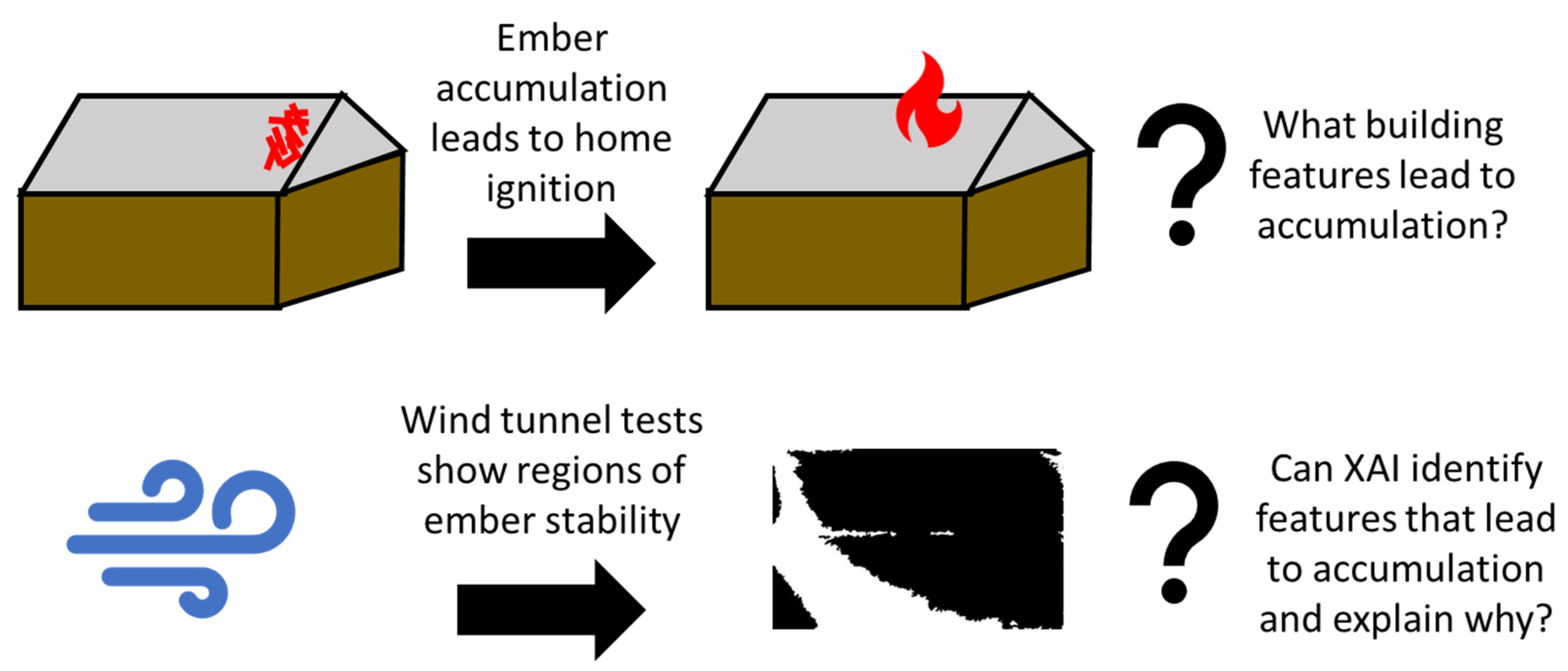
The literature shows that ember accumulation on buildings can lead to home ignition. This research addresses the overarching question, ‘what building features lead to accumulation of embers?’ Previously published wind tunnel experiments quantified where embers can remain in contact with a rooftop. Therefore, the specific research questions for this project are: ‘Can XAI identify building geometric features that lead to accumulation?’ and ‘can XAI explain why these features are important?’ See Figure 1 for a workflow diagram of this research project.
The results shown below demonstrate the following:
- The DL model is capable of accurately predicting the fraction of the roof that retains embers as a function of the building geometry and wind conditions;
- The XAI tools can identify the nature of the relationship between the ember coverage and the building and wind parameters;
- There is a distinct difference between the behavior on the windward and leeward retention processes that was elucidated by the XAI data.
The remainder of the paper is structured as follows. The experimental method used by [28] is briefly reviewed in Section 2, including a description of the parameter space tested and the image analysis tools used for data extraction. The DL model development and explainable AI tools used are described in Section 3. Model results are presented in Section 4, including a discussion of the model performance, explainable AI metrics, and limitations of the current study. Conclusions and suggestions for future directions are given in Section 5.
2. Experimental Methods
A series of experiments were carried out in the Clemson University atmospheric boundary layer wind tunnel with gable roof buildings with different roof slopes. The roof pitches used in the experiments were flat roofs and roofs with slopes of 2/12, 4/12, 6/12, and 10/12. The rooftops of the model houses were covered with model embers before exposing to the controlled wind load condition. The area of embers retained on the rooftop during and after experiments was tracked with a camera. These tracking images were then used for analysis.
2.1. Experimental Conditions
The flow similarity was carefully considered with both geometric and dynamic similarities to make sure that the lab-scale experiments modeled real-world problems. Geometric similarity was satisfied by matching the scale-down ratio for both model buildings and model embers. The model building was built with a geometric scale of 1/30. The model eave height was selected to be 10.1 cm (4 in) with a wall length of 20.3 cm (8 in) by 40.6 cm (16 in). This scaling ratio of 1/30 was selected to ensure that the cross-section area of the model building did not exceed 5% of the total wind tunnel cross-section area. This was to avoid the acceleration of the flow around the blockage generated by the building [43]. The resulting model building’s dimensions are shown in Figure 2 and Table 1. The model represents a full-scale building with plan dimensions of 6 m by 12 m (20′ by 40′) with a 3 m (10′) eave height.
Model embers were mass produced from pine straw. To satisfy the geometric similarity, model embers also needed to be scaled down at the same ratio as the model building, i.e., 1:30. To meet this scale down ratio, the model ember diameter had to be 0.16 mm and mass production was not practical for this study. The embers that were produced for this study had a mean length of 5 mm. The results of the embers retained on the rooftop presented in [28] proved that the size of the embers is significantly smaller than the size of the buildings and the retained ember area. Therefore, although the model ember sizes did not meet strict geometric similarity, the results could be reasonably extrapolated to full scale. The details of the ember production and the explanation of the satisfaction of the ember’s geometric similarity are presented in [28].
Dynamic similarity was met by equating non-dimensional force ratios at full and lab scale. The forces in this study are the aerodynamic forces on the house, the aerodynamic forces on the embers, the ember weight, and the friction between the embers and the roof material. The material of the fabric that was used to cover the rooftop of the model houses was selected to have the same friction coefficient as the shingle on the full-scale houses. This was to make sure that the model embers stayed in contact with the rooftops of the model houses under the wind load in a similar pattern as in the full-scale case. The process of testing the rooftop materials for the model houses is described in detail in [28], in which P60 sandpaper was chosen for covering the rooftop of model houses.
The similarity requirement of the aerodynamic forces on the houses should be satisfied by matching the Reynold number between full-scale and lab-scale experiments. However, this is not possible in boundary layer wind tunnels. However, according to [44], the flow becomes independent of the Reynolds number if it is larger than 7500. Therefore, provided the wind speed used in this study was greater than 1.1 m/s, we satisfied dynamic similarity for the flow over the model buildings.
In a similar way, the aerodynamic forces on the embers are dependent of the Reynold number, which is about 2000 for full-scale and approximately 140 for model embers. However, the drag coefficient for embers in the shape of cylinders with a length to diameter ratio of 8 is approximately constant over those Reynold numbers [45,46]. Although the Reynolds number matching was not satisfied, the drag coefficient was similar for both the full-scale and lab-scale scenarios.
Ember weight was reflected through the gravitation force, which is included in the non-dimensional Tachikawa number [47] as:
where is the density of air, is the wind speed at the eave height, is the ember material density, is gravitational acceleration, and is a characteristic length of the ember. Knowing the air density and the ember’s properties, the wind speeds in the experiments were adjusted based on the range of full-scale windspeed during an WUI fire to obtain the same K number for both full and lab scale.
2.2. Summary of Test Conditions
Six buildings were tested with an identical width of 20.3 cm (8 in), a length of 40.6 cm (16 in), and a height of 10.1 cm (4 in), but different roof pitches of 0/12 to 10/12 with 2/12 increments. The dimensions of these buildings are demonstrated in Figure 2 and are summarized in Table 1.
With each building listed in Table 1, the experiments were carried out with 7 different wind angles of 0, 15, 30, 45, 60, 75, and 90 degrees, where 0 degrees of wind direction is the case when the long side of the building is perpendicular to the flow, while 90 degrees is when the short side of the building is facing the wind flow. For each wind direction, each building was tested with 6 different wind speeds. The wind speed was measured at the eve height of the building. The wind speeds measured were 2.7, 3.1, 3.3, 3.5, 3.8, and 4.1 m/s (see Table 2). Hence, for each building listed in Table 1, there were 42 experiments (test conditions) (see Table 2).
2.3. Image Analysis
During each experiment, a camera was placed above the roof and was used to record the roof surface. This was then used to determine the area of the rooftop on which embers were retained. The experiment was ended when a visual observation confirmed that ember removal had stopped.
The image of the recording was then downloaded onto a computer and processed using the Matlab Image (MatLab R2023b) analysis toolbox. For each test condition (experiment), the image was cropped to show only the roof and then converted into a black and white image. The conversation was performed by applying an algorithm to differentiate the area covered by embers and the area of ember removal (see [28] for more details on this process). An example of an original image of the roof after an experiment and the black and white image is shown in Figure 3 below.
The area of retained embers on the roof was identified by a black color, where a black pixel has a value of 1 while the white pixel has a value of 0. Therefore, the total fractional area of retained embers on the rooftop can be quantified by summing the total value of the black pixels and dividing it by the total number of pixels in the image.
2.4. Qualitative Result
A total of 252 separate tests were conducted in this study for six roof slopes, seven wind directions, and six wind speeds. Some broad qualitative behaviors were observed. For example, it is clear that the ember removal was significantly impacted by the structure of the flow separation over the building. This can be seen in Figure 3, which shows significant ember removal along the path of the corner vortex that forms when the wind approaches a building at a 45° angle. It was also observed that increasing the roof slope did not always increase ember removal due to the flow separation over the roof ridge. A more detailed description of the experimental results is presented in [28], which presented data for the fraction of the entire roof surface on which embers were retained. However, while general results were discussed in [28], the paper does not develop a predictive model for ember retention and only addresses retention on the entire roof, despite the qualitative differences in ember retention on the windward and leeward sides of the rooftop. This paper seeks to address these shortcomings by breaking the experimental dataset into leeward and windward retention fractions and reanalyzing the data using deep learning techniques. The dataset analyzed consists of 504 separate roof segments with the retention fraction being controlled by the wind speed, wind angle, roof slope, and windward/leeward roof location.
3. Deep Learning (DL)
DL represents a subset of AI inspired by the human brain’s structure. The foundational work by McCulloch and Pitts in 1943 [48] laid the basics of understanding how the brain’s neuron’s function and since then has inspired the development of artificial neural networks (ANN). An ANN capitalizes on training neural networks with deep and fluid architectures to contain the unique structure of a series of processing layers. An ANN with multiple hidden layers can be formally termed a DL model.
A typical DL model consists of multiple layers of artificial neurons that process information by passing inputs through weighted sums and nonlinear activation functions. In each layer, each neuron receives input from all neurons in the preceding layer, forming a matrix-vector multiplication. Below is the general formula for a matrix-vector product, where is an (M × N) matrix, and the subscripts are the trained parameters of the preceding layers. From the above matrix multiplication, one can say that the output coming from the dense layer will be an N-dimensional vector.
Additionally, activation functions within these layers introduce nonlinearity, enabling the network to learn complex patterns and relationships in the data beyond what linear processes can achieve. Common activation functions include the Rectified Linear Unit (ReLU), which reduces the likelihood of vanishing gradients during training, thereby supporting deeper network architectures. The sigmoid function is another commonly used activation function that maps any input value to an output that ranges between 0 and 1, making it particularly suitable for tasks where the output is a probability or a fraction within this range. Figure 4 shows the above-mentioned activation functions’ identity functions. It should be noted that other examples of activation functions can be found elsewhere [49].
Finally, dropout layers can be critical in enhancing a DL model’s generalization capabilities, preventing overfitting [50]. In the dropout layer, a random subset of neurons is omitted during the training phase, which prevents the model from becoming overly dependent on any single feature and reduces the risk of overfitting. This technique effectively encourages the network to improve performance and reliability when exposed to new, unseen data. Together, dense layers, activation functions, and dropout layers constitute essential components that empower DL models to tackle various predictive modeling tasks.
3.1. Deep Learning Model Description
This section describes the development and validation of a DL model that can predict the accumulation of embers on a flat roof. This research utilized a comprehensive image database of ember accumulation on roofs conducted at Clemson University’s wind tunnel [28]. Subsequently, images were processed and analyzed to determine the total number of black and white pixels. The black pixels represent the accumulated embers, while the white pixels represent the areas from which embers were removed due to the imposed wind. The next step was building a DL model to predict the accumulation of embers based on the image analysis. Lastly, we implemented an explainability tool (i.e., SHAP) [42] to address the key factors influencing the accumulation of embers based on three scenarios.
- Using the complete ‘Full’ database of roof images, including leeward and windward sections;
- The database is segmented into two datasets based on the side feature;
- Lastly, the third segment of the windward dataset is selected for further examination.
In all three scenarios, the same model was initiated to observe the changes in the key influencing features and the changes in the roof settings on the accumulation of embers (which is tied to the possibility of ignition). Observing such changes offers explanations to better understand the DL model’s predictiveness, which, in turn, enhances the building’s fire safety and provides a safer roof setting to lessen the accumulation of embers on flat roofs.
3.2. Database Preprocessing
The collected database consisted of 504 roof images with various settings. Each image in the database illustrated ember accumulation under various features (conditions). Hence, the ember accumulation was selected as the target feature (output). The number of black pixels in the image represents the accumulation of embers (see Figure 3b). That is, the model did not take the images as its input but rather the fraction of the roof surface that remained covered with embers. The selected features as input included roof slopes, wind direction (denoted as an angle), wind speeds, and the side feature, which specifies whether the scenario was on the windward or leeward side of the roof.
The preprocessing stage started by importing and analyzing the images to extract the features from the images. Factors such as side, roof angle, and wind speed data were directly extracted from the source database using identifiable patterns related to the experimental setup. On the target (output) front, ember accumulation, the developed model calculated the accumulated embers on the rooftop by counting the number of black pixels in each roof image. The number of black pixels was then divided by the total number of pixels (white and black pixels) to normalize the target feature between 0–1. The above-mentioned extracted data were recorded and structured in matrix arrays as an input database for the model to make predictions.
3.3. Model Architecture
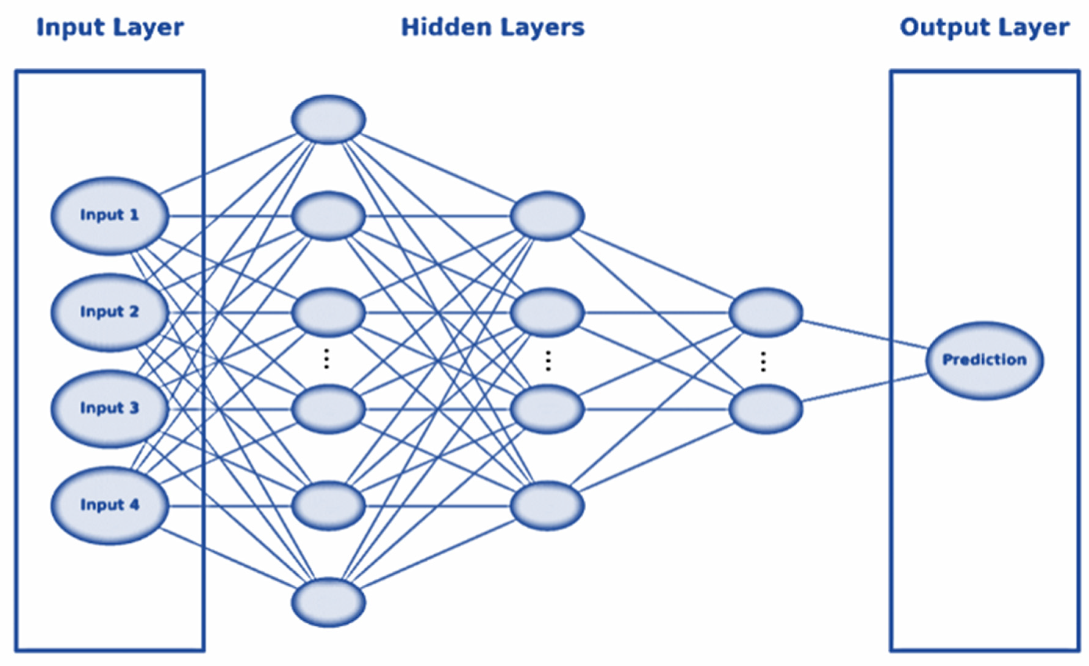
After a series of tuning steps, the designed DL model consisted of four dense layers, which allowed the model to learn and identify relationships between various features and the target label (the fraction of the roof surface covered in embers). The input dense layer contained 504 neurons with an input dimension mirroring the dimensionality of the input database and 128 for the leeward and windward datasets. Subsequent (hidden) layers were progressively smaller, with 64, 32, and 16 neurons respectively. Finally, the model architecture ended with a final dense layer with a single neuron, making a funnel-like ANN model structure for data processing—see Figure 5. The ‘ReLU’ activation function was selected for the input and hidden layers to introduce nonlinearity into the learning process. However, the ‘linear’ activation function was selected for the output layer since the target feature was a continuous fraction between 0 and 1 [51]. To combat overfitting, we implemented a dropout layer with a 20% rate to randomly ignore a subset of neurons during training.
3.4. Dataset Partitioning and Model Training and Evaluation
During the model’s training phase, a systematic analysis of selecting 200 epochs, with a batch size of five, provided the model with enough iterations to learn and balance the computational efficiency. Adopting the Adam optimizer [52,53], which is known for its adaptive learning rate properties, facilitates more accurate and practical model updates. This optimizer was instrumental in guiding the model toward an optimal set of weights, ensuring that each update was meaningful and conducive to the model’s overall learning curve.
The model’s performance was validated against a subset of the dataset to confirm the effectiveness of the learning process. This step was critical to ascertain that the model advanced beyond mere memorization of the training data. The dataset was divided into training and validation/testing sets, with a 70:30 ratio between the training and validation/testing data. It is noteworthy that the dataset was split using ‘sklearn train_test_split’ [54] in a random manner, with a condition of ensuring a non-changed data distribution. Upon completion of the training phase, the model’s predictions were evaluated against actual values in the validation set. The employed performance metrics were the coefficient of determination (R2) and the mean absolute error (MAE) [55,56,57]. The R2 score measures the quality of the model’s predictions of the actual data variance. The MAE, on the other hand, quantifies the average magnitude of errors in the predictions.
4. Results and Discussion
This section represents the outcomes of the data exploratory and XAI analyses. The discussion will focus on displaying the Pearson and Spearman correlation matrices. However, the ‘side’ feature is binary; hence, it will be discussed using the Point-biserial correlation. Subsequently, we focus on the model performance during the training, testing, and validating phases. Following that, we illustrate the results from the SHAP summary plots by focusing on the three segments of datasets used in this analysis, namely, the full images database, a second dataset that includes the leeward roof side of the images, and finally, the dataset that comprises only the windward side of the roof images.
4.1. Correlations
The Pearson correlation coefficients heatmap, which demonstrates the strength and direction of a linear relationship between the fraction of black pixels and all other features, is shown in Figure 6. This heatmap identifies which variables have the largest and lowest degrees of linear correlation with regard to the fraction of black pixels (fraction of the roof surface that retains embers), which is indicative of ember accumulation.
One can observe a mix of negative and positive correlations in the last row. The most notable negative correlation appears between wind speed and the fraction of accumulated embers, with a coefficient of −0.59. This strong inverse relationship suggests that increasing the wind speeds contributes to less ember accumulation. In addition, the coefficient between the roof slope and the fraction of black pixels is −0.35, indicating that the steeper roofs experience less ember accumulation. The correlation between the angle and the fraction of black pixels accounted for only −0.2, representing a relatively weak negative correlation. We opted not to discuss the ‘side’ feature in the Pearson correlation matrix because it can only be used for continuous features.
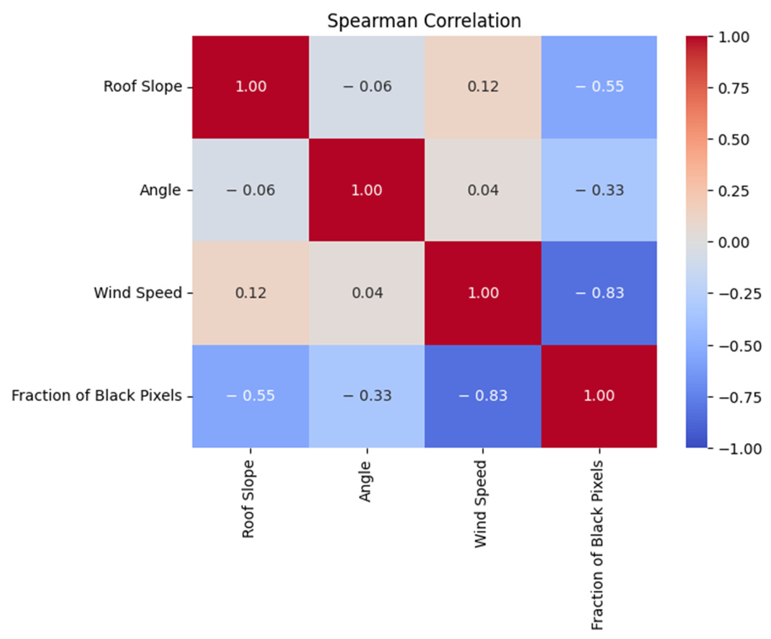
The Spearman correlation coefficients heatmap is shown in Figure 7. This shows the degree of monotonic relationship between the fraction of black pixels and the other features. Similar to the Pearson correlation coefficient, the most significant negative correlation is between wind speed and the fraction of black pixels, accounting for around −0.83. The roof slope accounted for a Spearman correlation of −0.55 with the fraction of black pixels, suggesting that roofs with greater slopes tend to have less ember accumulation, which is in line with the monotonic but not necessarily linear trend this measure captures. The angle presents a milder negative Spearman correlation of −0.33 with the fraction of black pixels, indicating a less strong yet inverse relationship. Like the Pearson correlation, the Spearman correlation heatmap cannot be used for binary features; hence, it will be discussed in the Point-biserial correlation. A cross-examination between the Spearman and Pearson correlation matrices shows that the Spearman coefficient is higher in magnitude than the Pearson’s.
Lastly, the Point-biserial correlation is a special case of the Pearson correlation that can be applied when one variable is categorical with two categories, and the other data are continuous. As seen in Figure 8, the heatmap shows a positive correlation of 0.24 between the leeward side variable and the fraction of black pixels and a negative −0.24 for the windward side. Moreover, the leeward side is the only positive correlation observed, which indicates an increase in ember accumulation on the side of the structure that does not face the wind compared to the windward side.
4.2. Model Evaluation
This section presents the model evaluation process. First, a visual comparison through a line plot, illustrating the model’s predictions versus actual outcomes, was applied to the full database to evaluate the overall predictive performance. Then, we utilized two evaluation metrics: R-squared (R2) and mean absolute error (MAE). These metrics were adopted to evaluate the model performance for predicting ember accumulation on roofs. Lastly, in addition to the full database, these metrics were implemented into the model to provide insight into the accuracy and precision of our model across the leeward and windward datasets.
4.2.1. Full Database Model Performance
Figure 9 visually illustrates the model’s prediction versus the actual outcome. As one can see, the model accurately predicted the fraction of ember coverage (represented by the black pixels). In addition, the R2 evaluation metric showed a value of 95.5%, which signifies a high level of accuracy. This indicates that the model can predict the fraction of black pixels within 95.5% of the original fraction of ember accumulation. Similarly, the MAE showed a 0.05 error, representing the average magnitude of the errors in the model’s predictions. This combination of a high R2 and a low MAE demonstrates the model’s robust predictive capability, making it a potentially valuable tool for applications requiring precise ember accumulation forecasts.
4.2.2. Leeward and Windward Datasets
The model’s results varied when segmenting the database into two segments based on the side feature, whether the images were for the leeward or the windward roof section. On the leeward front, the R2 accuracy remained stable at around 93.4%, and the MAE dropped slightly to 0.050. Alternatively, the windward dataset’s R2 accuracy dropped to around 87.7%. In addition, the MAE evaluation showed an increase in error to 0.08.
Notably, the training evaluation metrics followed a similar trend to the testing results, with the complete database dropping slightly, which can be explained by the considerable number of samples the model used for training. Table 3 tabulates the training and testing/validating evaluation metrics for the original database and the segmented datasets.
4.2.3. SHAP Explainability Tools
The second goal of this study was to identify the impact of the selected parameters on roof ember accumulation by utilizing the SHAP explainability tool [42]. SHAP is a model-agnostic tool designed to provide an explainable layer to AI models, which are typically black boxes because users cannot observe how such models reached a prediction. SHAP offers a visual representation of how much each selected feature contributes to the model’s final prediction and the direction of its impact.
More specifically, such an explainability tool achieves both broad and detailed interpretations by calculating Shapley values, which consider every combination and interaction between features in the database rather than directly using the database features [58]. Shapley values are based on game theory, which requires two essential parts, namely, the ‘game’ and the ‘players’, where each player is a feature, and each game is a prediction. The ‘game’ represents the model’s outcome, while the players represent the database features. Shapley values quantify the impact of each player on the game, or in other words, each feature’s contribution to a prediction.
In regression models, to calculate the effect of a feature on prediction, Shapley values require training the model in all feature subsets as shown in Table 4 [42]. To determine that specific feature effect, the model is trained using that specific feature, and then another model is trained on another feature. Subsequently, based on the input, comparisons are to be made between predictions from the two associated models . This comparison accounts for the fact that the impact of excluding a feature is influenced by the presence of other features in the model. Such differences are calculated for every subset of features, Shapley values are subsequently derived, and the average is taken and utilized as feature importance.
SHAP generates a holistic (global) understanding and investigates the impact of each feature on the model’s target feature via SHAP summary plot. It is typically illustrated as a dot plot, where each point represents a Shapley value for a feature and an instance. Features are listed on the y-axis, arranged by their overall importance (usually determined by the sum of SHAP value magnitudes across all instances). The graph organizes these factors in descending order, starting with the most influential contributor and moving down to the least, according to their effect on the model’s output. The x-axis represents the Shapley values, indicating how each feature contributes to shifting the model output from the base point.
Moreover, the summary plot added a new layer to determine the direction of the impact of the feature on the model prediction. The color coding of dots provides that additional layer where high feature values, represented by red dots, contribute to higher predictions. In addition, the density of the dots across the x-axis can also inform about the variability of a feature’s effect. A wide spread of dots across the Shapley values range indicates a significant impact on the prediction, while a narrow spread suggests a lower influence. This section demonstrates the results obtained from implementing the SHAP explainability tool by means of a summary plot into the DL model.
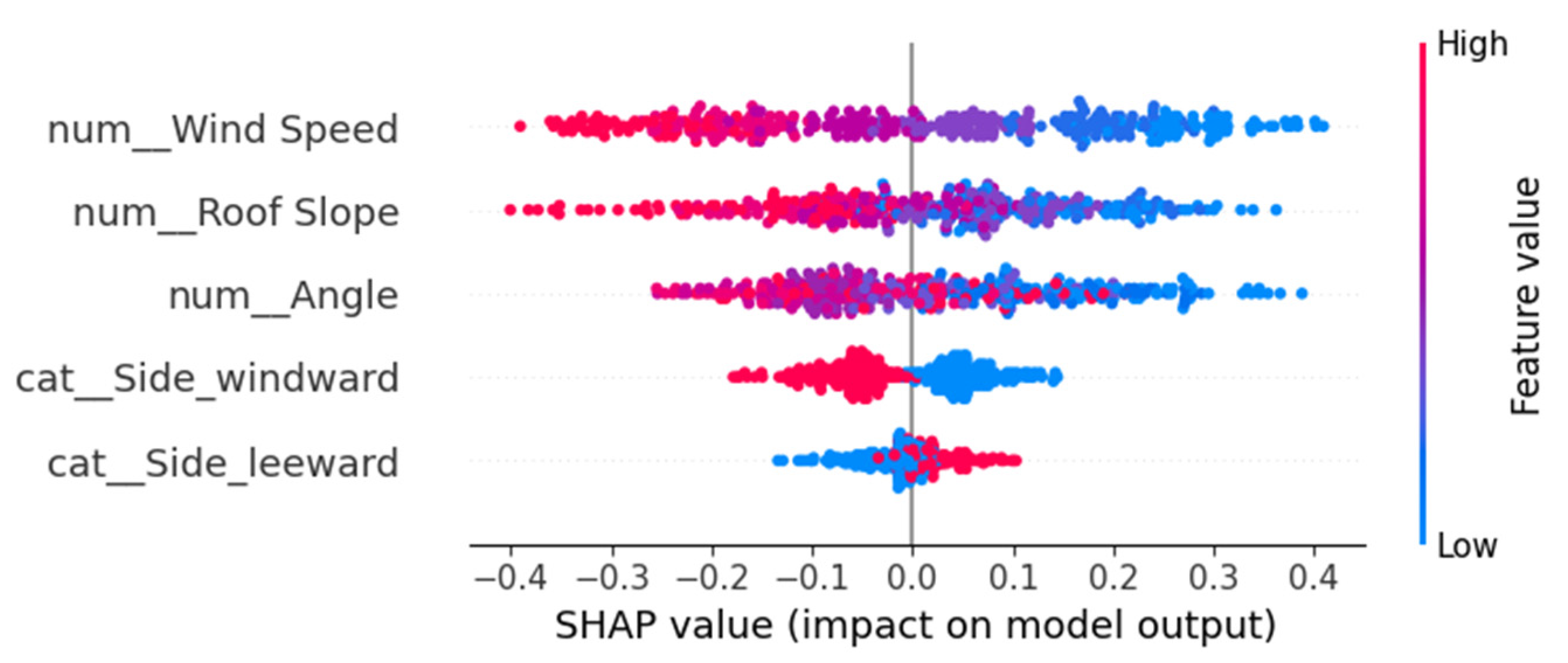
Figure 10 shows that wind speed was the most critical feature contributing to the prediction, followed by the roof slope and wind angle. In addition, the windward and leeward categories were the lowest contributors to the predictions. On the color-coding front, all the top three influencing features showed that higher values [represented by the red dots] of these features contributed to decreasing the fraction of black pixels. Moreover, lower values [represented by blue dots] were associated with a higher accumulation of embers in the fraction of black pixels. This is consistent with the correlation coefficients data in Figure 6 and Figure 7, which show that all these parameters were negatively correlated with ember coverage.
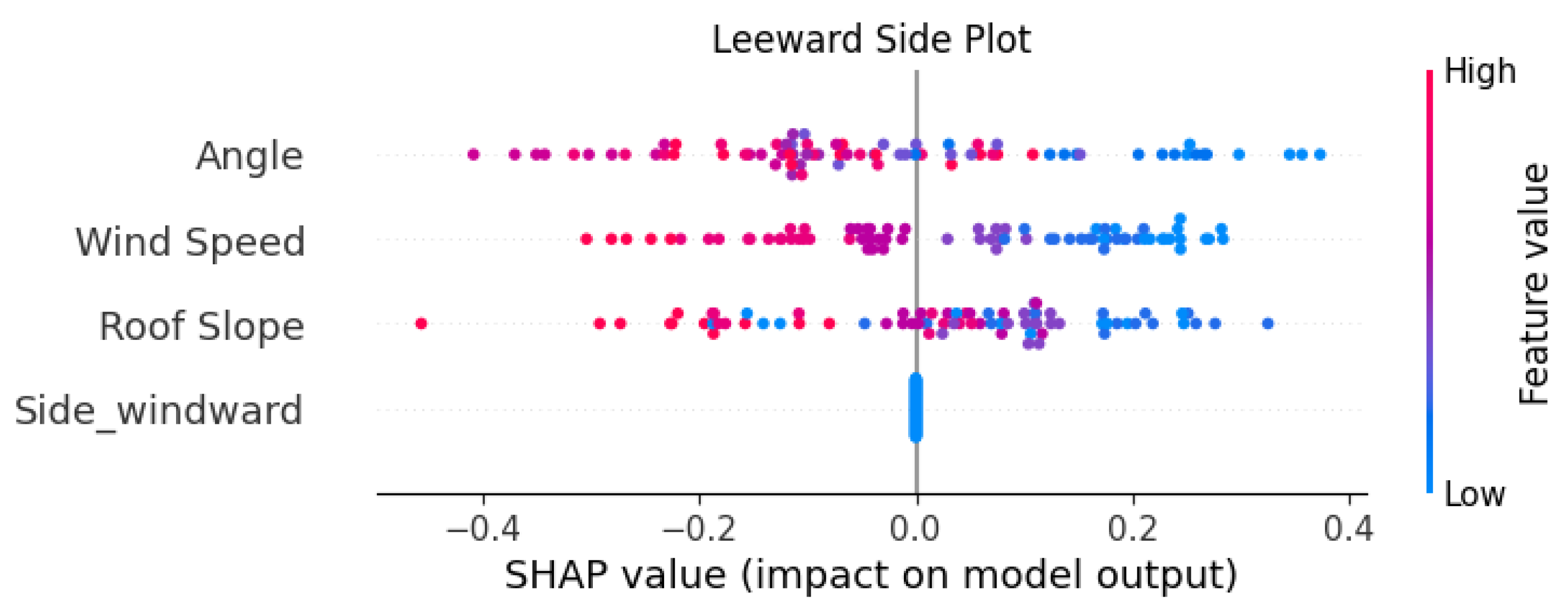
The SHAP summary plots for the separated windward and leeward datasets are shown in Figure 11. A comparison of the two SHAP summary plots highlights some key differences between the ember retention on the windward and leeward sides of the rooftop. First, wind speed played the largest role in the model prediction for the windward side, followed by roof slope and wind angle. Moreover, the roof slope played the largest role for the leeward side, followed by wind speed and wind angle. This is consistent with the theory suggested in [28], which states that the flow separation along the eaves and roof ridge controls ember removal. For the roof’s leeward side, the flow structure was controlled by the flow separation along the ridge and was, therefore, significantly influenced by the roof slope at the ridgeline.
A second interesting distinction is that the wind angle played a much larger role in the ember retention on the leeward side compared to the windward side. All but three SHAP values for the windward side range between , whereas for the leeward side of the roof, the values range from −0.3 to +0.35. This is again consistent with the flow separation theory. The structure of the wind flow on the leeward side of the roof is controlled by the roof ridge angle and the wind angle relative to the ridge line. It is also worth noting that, on the windward side, many of the large wind angles (red dots) have positive SHAP values, whereas predominantly small wind angles (blue dots) have positive SHAP values. Again, this suggests that the retention process on the leeward side of the rooftop is qualitatively and quantitatively different. This is not clear from the summary model quality statistics presented in Table 3 and is only shown through a detailed analysis of the SHAP summary plots.
The results above demonstrate the power of this approach to quantify ember retention on rooftops during WUI fires and the value of XAI tools for elucidating behaviors that influence ember retention. However, there is more work needed before this tool can be of general use in home fire risk assessment. The limitations of the present study are as follows:
- This work is limited to rectangular floor plan buildings with sloped gable end roofs and does not account for complex roof shapes. This is due, in part, to the lack of experimental data for non-rectangular roof buildings. Once building shapes beyond rectangular are considered, there is a significant increase in the number of parameters. For example, simply adding a T-shaped building introduces internal and external roof corners. There are geometric features that have only one dimension (length) and so much more work would need to be done to assess the influence area of such features. This would require a much larger dataset of non-rectangular buildings than is currently unavailable;
- In general, complicating the roof types/shapes will increase the complexity of the DL model, which will dramatically increase the already significant computational resources required for training and testing;
- Although some explainability tools can be implemented in ANN to extract qualitative insights and verify domain knowledge, quantified interpretability remains a challenge. That is, the XAI data must still be interpreted with a domain expert to gain the full benefit of the analysis.
5. Conclusions
A DL model was used to develop a predictive model for identifying the fraction of a roof surface that is susceptible to ember accumulation during a WUI fire. The experimental data of [28] were used as the data source for both training and testing the developed model. The model was trained and tested on the full dataset and on subsets of the dataset to distinguish between the windward and leeward halves of the roof. Global measures of the quality of fit were used to assess the model performance. Both the R2 and MAE parameters showed very good performance for the model for both the full dataset and the two halves of the dataset analyzed separately.
Explainability tools (XAI) were then applied to provide insights into the workings of the model. The SHAP summary plot for the entire dataset shows that the wind speed is the biggest contributor to the model prediction and, consistent with the Pearson and Spearman correlation heat maps in Figure 6 and Figure 7, the fraction of the rooftop on which embers are retained is negatively correlated with the magnitude of the wind speed. When the dataset was segmented into windward and leeward halves, the SHAP summary charts were qualitatively and quantitatively different. In particular, the wind angle plays a much larger role in ember retention on the leeward side of the rooftop. This is consistent with the theory that the flow structure is controlled by the flow separation along the eaves and roof ridge and, therefore, that the incident angle between the ridge and the wind is key to controlling ember retention. This suggests that the AI model is capturing some subtle features of the flow behavior and ember removal process.
The application of DL and XAI to ember accumulation provides both accurate quantitative predictions of the fraction of the rooftop on which embers can accumulate and insights into the mechanisms that allow embers to remain in contact with the roof surface. One drawback of the current study is that the dataset consists only of rectangular floor plan buildings with sloped gable end roofs. In the future, this work should be expanded to include more complex building floor plans and roof shapes. While limited experimental data in the literature [28] can be used to train and test such a model, the size of the datasets available would limit the accuracy of the model. Additional experiments are required to expand this dataset. Furthermore, work needs to be done to develop metrics for quantifying various roof features, such as dormer windows and internal corners, before they could be implemented into the model presented herein.
Author Contributions
Conceptualization: N.B.K., M.K.A.-B., M.Z.N. and D.N.; Methodology M.Z.N. and M.K.A.-B.; Data curation: D.N.; Analysis: M.K.A.-B. and M.Z.N.; Resources: N.B.K.; Writing, review, and editing: N.B.K., M.K.A.-B., D.N. and M.Z.N.; Funding Acquisition: N.B.K. All authors have read and agreed to the published version of the manuscript.
Funding
This work was performed under the following financial assistance award 70NANB17H213 from the US Department of Commerce, National Institute of Standards and Technology.
Institutional Review Board Statement
Not applicable.
Informed Consent Statement
Not applicable.
Data Availability Statement
Data are contained within the article.
Conflicts of Interest
The authors declare no conflict of interest.
References
- Mckenzie, D.; Littell, J.S. Climate change and the eco-hydrology of fire: Will area burned increase in a warming western USA? Ecol. Appl. 2017, 27, 26–36. [Google Scholar] [CrossRef] [PubMed]
- Abatzoglou, J.T.; Kolden, C.A. Climate Change in Western US Deserts: Potential for Increased Wildfire and Invasive Annual Grasses. Rangel. Ecol. Manag. 2011, 64, 471–478. [Google Scholar] [CrossRef]
- Pinol, J.; Terradas, J.; Lloret, F. Climate warming, wildfire hazard, and wildfire occurrence in coastal eastern Spain. Clim. Change 1998, 38, 345–357. [Google Scholar] [CrossRef]
- Cal Fire. Top 20 Deadliest California Wildfires. Available online: https://www.fire.ca.gov/our-impact/statistics (accessed on 12 December 2023).
- National Museum of Australia, National Museum of Australia—Black Saturday Bushfires. Available online: https://www.nma.gov.au/defining-moments/resources/black-saturday-bushfires (accessed on 12 December 2023).
- Unprecedented season breaks all records. Bush Fire Bull. 2020, 42, 2–4. Available online: https://www.rfs.nsw.gov.au/__data/assets/pdf_file/0007/174823/Bush-Fire-Bulletin-Vol-42-No1.pdf (accessed on 12 December 2023).
- Mell, W.E.; Manzello, S.L.; Maranghides, A.; Butry, D.; Rehm, R.G. The wildland–urban interface fire problem—Current approaches and research needs. Int. J. Wildland Fire 2010, 19, 238–251. [Google Scholar] [CrossRef]
- Manzello, S.L.; Suzuki, S.; Gollner, M.J.; Fernandez-Pello, A.C. Role of firebrand combustion in large outdoor fire spread. Prog. Energy Combust. Sci. 2020, 76, 100801. [Google Scholar] [CrossRef] [PubMed]
- Koo, E.; Pagni, P.J.; Weise, D.R.; Woycheese, J.P. Firebrands and spotting ignition in large-scale fires. Int. J. Wildland Fire 2010, 19, 818–843. [Google Scholar] [CrossRef]
- Manzello, S.L.; Maranghides, A.; Mell, W.E. Firebrand generation from burning vegetation. Int. J. Wildland Fire 2007, 16, 458–462. [Google Scholar] [CrossRef]
- Mell, W.; Maranghides, A.; McDermott, R.; Manzello, S.L. Numerical simulation and experiments of burning Douglas fir trees. Combust. Flame 2009, 156, 2023–2041. [Google Scholar] [CrossRef]
- Sayaka, S.; Manzello, S.L. Firebrand production from building components fitted with siding treatments. Fire Saf. J. 2016, 80, 64–70. [Google Scholar]
- Manzello, S.L.; Suzuki, S. Generating wind-driven firebrand showers characteristic of burning structures. Proc. Combust. Inst. 2017, 36, 3247–3252. [Google Scholar] [CrossRef] [PubMed]
- Tohidi, A.; Kaye, N.B.; Bridges, W. Statistical description of firebrand size and shape distribution from coniferous trees for use in Metropolis Monte Carlo simulations of firebrand flight distance. Fire Saf. J. 2015, 77, 21–35. [Google Scholar] [CrossRef]
- Albini, F.A. Transport of firebrands by line thermals. Combust. Sci. Technol. 1983, 32, 277–288. [Google Scholar] [CrossRef]
- Anthenien, R.A.; Tse, S.D.; Fernandez-Pello, A.C. On the trajectories of embers initially elevated or lofted by small scale ground fire plumes in high winds. Fire Saf. J. 2006, 41, 349–363. [Google Scholar] [CrossRef]
- Bhutia, S.; Jenkins, M.A.; Sun, R. Comparison of firebrand propagation prediction by a plume model and a coupled-fire/atmosphere large-eddy simulator. J. Adv. Model. Earth Syst. 2010, 2, 4. [Google Scholar] [CrossRef]
- Tohidi, A.; Kaye, N.B. Stochastic modeling of firebrand shower scenarios. Fire Saf. J. 2017, 91, 91–102. [Google Scholar] [CrossRef]
- Tohidi, A.; Kaye, N.B. Comprehensive wind tunnel experiments of lofting and downwind transport of non-combusting rod-like model firebrands during firebrand shower scenarios. Fire Saf. J. 2017, 90, 95–111. [Google Scholar] [CrossRef]
- Wadhwani, R.; Sutherland, D.; Ooi, A.; Moinuddin, K. Firebrand transport from a novel firebrand generator: Numerical simulation of laboratory experiments. Int. J. Wildland Fire 2022, 31, 634–648. [Google Scholar] [CrossRef]
- Standohar-Alfano, C.D.; Estes, H.; Johnston, T.; Morrison, M.J.; Brown-Giammanco, T.M. Reducing Losses from Wind-Related Natural Perils: Research at the IBHS Research Center. Front. Built Environ. 2017, 3, 9. [Google Scholar] [CrossRef]
- Suzuki, S.; Manzello, S.L. Experimental investigation of firebrand accumulation zones in front of obstacles. Fire Saf. J. 2017, 94, 1–7. [Google Scholar] [CrossRef]
- Suzuki, S.; Johnsson, E.; Maranghides, A.; Manzello, S. Ignition of wood fencing assemblies exposed to continuous wind-driven firebrand showers. Fire Technol. 2016, 52, 1051–1067. [Google Scholar] [CrossRef]
- Manzello, S.; Suzuki, S.; Nii, D. Full-scale experimental investigation to quantify building component ignition vulnerability from mulch beds attacked by firebrand showers. Fire Technol. 2017, 53, 535–551. [Google Scholar] [CrossRef] [PubMed]
- Stephen, L.Q.; Christine, S.-A.; Faraz, H.; Daniel, J.G. Factors influencing ember accumulation near a building. Int. J. Wildland Fire 2023, 32, 80–387. [Google Scholar]
- Nguyen, D.; Kaye, N.B. Quantification of ember accumulation on the rooftops of isolated buildings in an ember storm. Fire Saf. J. 2022, 128, 103525. [Google Scholar] [CrossRef]
- Nguyen, D.; Kaye, N.B. The role of surrounding buildings on the accumulation of embers on rooftops during an ember storm. Fire Saf. J. 2022, 131, 103624. [Google Scholar] [CrossRef]
- Nguyen, D.; Kaye, N.B. Experimental investigation of rooftop hotspots during wildfire ember storms. Fire Saf. J. 2021, 125, 103445. [Google Scholar] [CrossRef]
- Jain, P.; Coogan, S.C.P.; Subramanian, S.G.; Crowley, M.; Taylor, S.; Flannigan, M.D. A review of machine learning applications in wildfire science and management. Environ. Rev. 2020, 28, 478–505. [Google Scholar] [CrossRef]
- Aikaterini-Eleni, L. Wildfire Prediction Using Machine Learning; University of West Attica Institutional Repository: Athens, Greece, 2022. [Google Scholar] [CrossRef]
- Storer, J.; Green, R. PSO Trained Neural Networks for predicting forest fire size: A comparison of implementation and performance. In Proceedings of the International Joint Conference on Neural Networks, Vancouver, Canada, 24–29 July 2016; pp. 676–683. [Google Scholar] [CrossRef]
- Lall, S.; Mathibela, B. The Application of Artificial Neural Networks for Wildfire Risk Prediction. In Proceedings of the International Conference on Robotics and Automation, Stockholm, Sweden, 16–21 May 2016; Available online: https://0-ieeexplore-ieee-org.brum.beds.ac.uk/abstract/document/7931880/ (accessed on 23 February 2024).
- Li, L.-M.; Song, W.-G.; Ma, J.; Satoh, K. Artificial neural network approach for modeling the impact of population density and weather parameters on forest fire risk. Int. J. Wildland Fire 2009, 18, 640–647. [Google Scholar] [CrossRef]
- Xiong, Y.; Wu, J.; Chen, Z. Machine Learning Wildfire Prediction Based on Climate Data. Available online: http://noiselab.ucsd.edu/ECE228-2020/projects/Report/75Report.pdf (accessed on 23 February 2024).
- Sakr, G.; Elhajj, I.; Mitri, G. Efficient forest fire occurrence prediction for developing countries using two weather parameters. Eng. Appl. Artif. Intell. 2011, 24, 888–894. [Google Scholar] [CrossRef]
- Vecín-Arias, D.; Castedo-Dorado, F.; Ordóñez, C.; Rodríguez-Pérez, J.R. Biophysical and lightning characteristics drive lightning-induced fire occurrence in the central plateau of the Iberian Peninsula. Agric. For. Meteorol. 2016, 225, 36–47. [Google Scholar] [CrossRef]
- Preeti, T.; Kanakaraddi, S.; Beelagi, A.; Malagi, S.; Sudi, A. Forest Fire Prediction Using Machine Learning Techniques. In Proceedings of the 2021 International Conference on Intelligent Technologies, CONIT 2021, Hubli, India, 25–27 June 2021. [Google Scholar] [CrossRef]
- Aldersley, A.; Murray, S.; Cornell, S. Global and regional analysis of climate and human drivers of wildfire. Sci. Total. Environ. 2011, 409, 3472–3481. [Google Scholar] [CrossRef] [PubMed]
- Cortez, P.; Morais, A. A Data Mining Approach to Predict Forest Fires Using Meteorological Data. 2007. Available online: https://repositorium.sdum.uminho.pt/handle/1822/8039 (accessed on 23 February 2024).
- Guo, F.; Zhang, L.; Jin, S.; Tigabu, M.; Su, Z.; Wang, W. Modeling Anthropogenic Fire Occurrence in the Boreal Forest of China Using Logistic Regression and Random Forests. Forests 2016, 7, 250. [Google Scholar] [CrossRef]
- Xie, Y.; Peng, M. Forest fire forecasting using ensemble learning approaches. Neural Comput. Appl. 2019, 31, 4541–4550. [Google Scholar] [CrossRef]
- Lundberg, S.; Lee, S.-I. A Unified Approach to Interpreting Model Predictions. In Proceedings of the 31st International Conference on Neural Information Processing Systems, Long Beach, CA, USA, 4–9 December 2017; pp. 4768–4777. [Google Scholar]
- American Society of Civil Engineers. Wind Tunnel Testing for Buildings and Other Structures: ASCE/SEI 49-12; American Society of Civil Engineers: Reston, VA, USA, 2012. [Google Scholar]
- Meroney, R.N.; Pavageau, M.; Rafailidis, S.; Schatzmann, M. Study of line source characteristics for 2-D physical modelling of pollutant dispersion in street canyons. J. Wind. Eng. Ind. Aerodyn. 1996, 62, 37–56. [Google Scholar] [CrossRef]
- Hoerner, S.F. Fluid-Dynamic Drag: Practical Information on Aerodynamic Drag and Hydrodynamic Resistance; Liselotte A. Hoerner: Bakersfield, CA, USA, 1965. [Google Scholar]
- Knudsen, J.G.; Katz, D.L. Fluid Dynamics and Heat Transfer; McGraw-Hill: New York, NY, USA, 1958. [Google Scholar]
- Holmes, H.D.; Baker, C.J.; Tamura, Y. Tachikawa number: A proposal. J. Wind. Eng. Ind. Aerodyn. 2006, 94, 41–47. [Google Scholar] [CrossRef]
- McCulloch, W.S.; Pitts, W. A logical calculus of the ideas immanent in nervous activity. Bull. Math. Biophys. 1943, 5, 115–133. [Google Scholar] [CrossRef]
- Lau, M.M.; Lim, K.H. Review of Adaptive Activation Function in Deep Neural Network. In Proceedings of the 2018 IEEE-EMBS Conference on Biomedical Engineering and Sciences (IECBES), Sarawak, Malaysia, 3–6 December 2018; pp. 686–690. [Google Scholar] [CrossRef]
- Srivastava, N.; Hinton, G.; Krizhevsky, A.; Salakhutdinov, R. Dropout: A Simple Way to Prevent Neural Networks from Overfitting. J. Mach. Learn. Res. 2024, 15, 1929–1958. [Google Scholar]
- Pratiwi, H.; Windarto, A.P.; Susliansyah, S.; Aria, R.R.; Susilowati, S.; Rahayu, L.K.; Fitriani, Y.; Merdekawati, A.; Rahadjeng, I.R. Sigmoid Activation Function in Selecting the Best Model of Artificial Neural Networks. J. Phys. Conf. Ser. 2020, 1471, 012010. [Google Scholar] [CrossRef]
- Adam. Available online: https://keras.io/api/optimizers/adam/ (accessed on 25 February 2024).
- Sumera, S.; Sirisha, R.; Anjum, N.; Vaidehi, K. Implementation of CNN and ANN for Fashion-MNIST-Dataset using Different Optimizers. Indian J. Sci. Technol. 2022, 15, 2639–2645. [Google Scholar] [CrossRef]
- Pedregosa, F.; Varoquaux, G.; Gramfort, A.; Michel, V.; Thirion, B.; Grisel, O.; Blondel, M.; Prettenhofer, P.; Weiss, R.; Dubourg, V.; et al. Scikit-learn: Machine Learning in Python. J. Mach. Learn. Res. 2011, 12, 2825–2830. [Google Scholar]
- Pahlavani, P.; Raei, A.; Bigdeli, B.; Ghorbanzadeh, O. Identifying Influential Spatial Drivers of Forest Fires through Geographically and Temporally Weighted Regression Coupled with a Continuous Invasive Weed Optimization Algorithm. Fire 2024, 7, 33. [Google Scholar] [CrossRef]
- Labres dos Santos, J.F.; Kovalsyki, B.; Ferreira, T.d.S.; Batista, A.C.; Tetto, A.F. Adjustment of the Grass Fuel Moisture Code for Grasslands in Southern Brazil. Fire 2022, 5, 209. [Google Scholar] [CrossRef]
- Naser, M.Z.; Alavi, A.H. Error Metrics and Performance Fitness Indicators for Artificial Intelligence and Machine Learning in Engineering and Sciences. Archit. Struct. Constr. 2023, 3, 499–517. [Google Scholar] [CrossRef]
- Shapley, L.S. A Value for n-Person Games. In Contributions to the Theory of Games (AM-28); Princeton University Press: Princeton, NJ, USA, 2016; Volume II, pp. 307–318. [Google Scholar] [CrossRef]
Figure 1.
Flow diagram of research project showing motivation, experimental work, and research questions.
Figure 1.
Flow diagram of research project showing motivation, experimental work, and research questions.

Figure 2.
Diagram of the model building’s dimensions. The specific values for each dimension are given in Table 1.
Figure 2.
Diagram of the model building’s dimensions. The specific values for each dimension are given in Table 1.

Figure 3.
Roof image of retained embers. (a) Original image; (b) after processing, where black pixels indicate the presence of embers retained on the rooftop. For this experiment, the wind was approaching at a 45° angle from the upper-left corner of the building.
Figure 3.
Roof image of retained embers. (a) Original image; (b) after processing, where black pixels indicate the presence of embers retained on the rooftop. For this experiment, the wind was approaching at a 45° angle from the upper-left corner of the building.

Figure 4.
Commonly used activation functions.

Figure 5.
Illustration of a typical DL model, including one input layer, four hidden layers, and one output layer. Note: input features include wind speed, wind direction, roof slope, and location.
Figure 5.
Illustration of a typical DL model, including one input layer, four hidden layers, and one output layer. Note: input features include wind speed, wind direction, roof slope, and location.

Figure 6.
Pearson correlation heatmap.

Figure 7.
Spearman correlation heatmap.

Figure 8.
Point-biserial correlation heatmap.

Figure 9.
An illustration of the accuracy of the model prediction. The red line represents exact agreement.
Figure 9.
An illustration of the accuracy of the model prediction. The red line represents exact agreement.

Figure 10.
Summary plot of Shapley values for the full database.

Figure 11.
Summary plot of Shapley values for the windward (top) and leeward (bottom) datasets.


Table 1.
Summary of the geometry of tested buildings.
| House | cm | cm | cm | cm | Roof Pitch |
|---|---|---|---|---|---|
| A | 10.1 | 20.3 | 40.6 | 0 | 0/12 |
| B | 10.1 | 20.3 | 40.6 | 1.7 | 2/12 |
| C | 10.1 | 20.3 | 40.6 | 3.4 | 4/12 |
| D | 10.1 | 20.3 | 40.6 | 5.1 | 6/12 |
| E | 10.1 | 20.3 | 40.6 | 6.8 | 8/12 |
| F | 10.1 | 20.3 | 40.6 | 8.5 | 10/12 |
Table 2.
Tested condition for each roof pitch.
| Wind Angle (Degrees) | Wind Speed (m/s) |
|---|---|
| 0, 15, 30, 45, 60, 75, and 90 | 2.7, 3.1, 3.3, 3.5, 3.8, and 4.1 |
Table 3.
Comparison of the evaluation metrics for the three segments of datasets.
| Evaluation Metric | Full | Leeward | Windward | Full | Leeward | Windward |
|---|---|---|---|---|---|---|
| Training | Testing/Validation | |||||
| R2 | 98.8% | 99.2% | 99.2% | 95.5% | 93.4% | 87.7% |
| MAE | 0.025 | 0.023 | 0.02 | 0.050 | 0.056 | 0.077 |
Table 4.
Summary of Shapley value calculations used in the XAI models [42].
Table 4.
Summary of Shapley value calculations used in the XAI models [42].
| SHAP |
|---|
| : set of the selected features; s: the values of the input features in the set S. |S|!: the number of permutations of feature values that appear before i-th feature value. (|M| − |S| − 1)!: the number of permutations of feature values that appear after the i-th feature value. |
Note: The difference term in (|M| − |S| − 1)! is the marginal contribution of adding the i-th feature value to S.
Disclaimer/Publisher’s Note: The statements, opinions and data contained in all publications are solely those of the individual author(s) and contributor(s) and not of MDPI and/or the editor(s). MDPI and/or the editor(s) disclaim responsibility for any injury to people or property resulting from any ideas, methods, instructions or products referred to in the content. |
© 2024 by the authors. Licensee MDPI, Basel, Switzerland. This article is an open access article distributed under the terms and conditions of the Creative Commons Attribution (CC BY) license (https://creativecommons.org/licenses/by/4.0/).
Share and Cite
MDPI and ACS Style
Al-Bashiti, M.K.; Nguyen, D.; Naser, M.Z.; Kaye, N.B. Predicting Wildfire Ember Hot-Spots on Gable Roofs via Deep Learning. Fire 2024, 7, 153. https://0-doi-org.brum.beds.ac.uk/10.3390/fire7050153
AMA Style
Al-Bashiti MK, Nguyen D, Naser MZ, Kaye NB. Predicting Wildfire Ember Hot-Spots on Gable Roofs via Deep Learning. Fire. 2024; 7(5):153. https://0-doi-org.brum.beds.ac.uk/10.3390/fire7050153
Chicago/Turabian StyleAl-Bashiti, Mohammad Khaled, Dac Nguyen, M. Z. Naser, and Nigel B. Kaye. 2024. "Predicting Wildfire Ember Hot-Spots on Gable Roofs via Deep Learning" Fire 7, no. 5: 153. https://0-doi-org.brum.beds.ac.uk/10.3390/fire7050153