1. Introduction
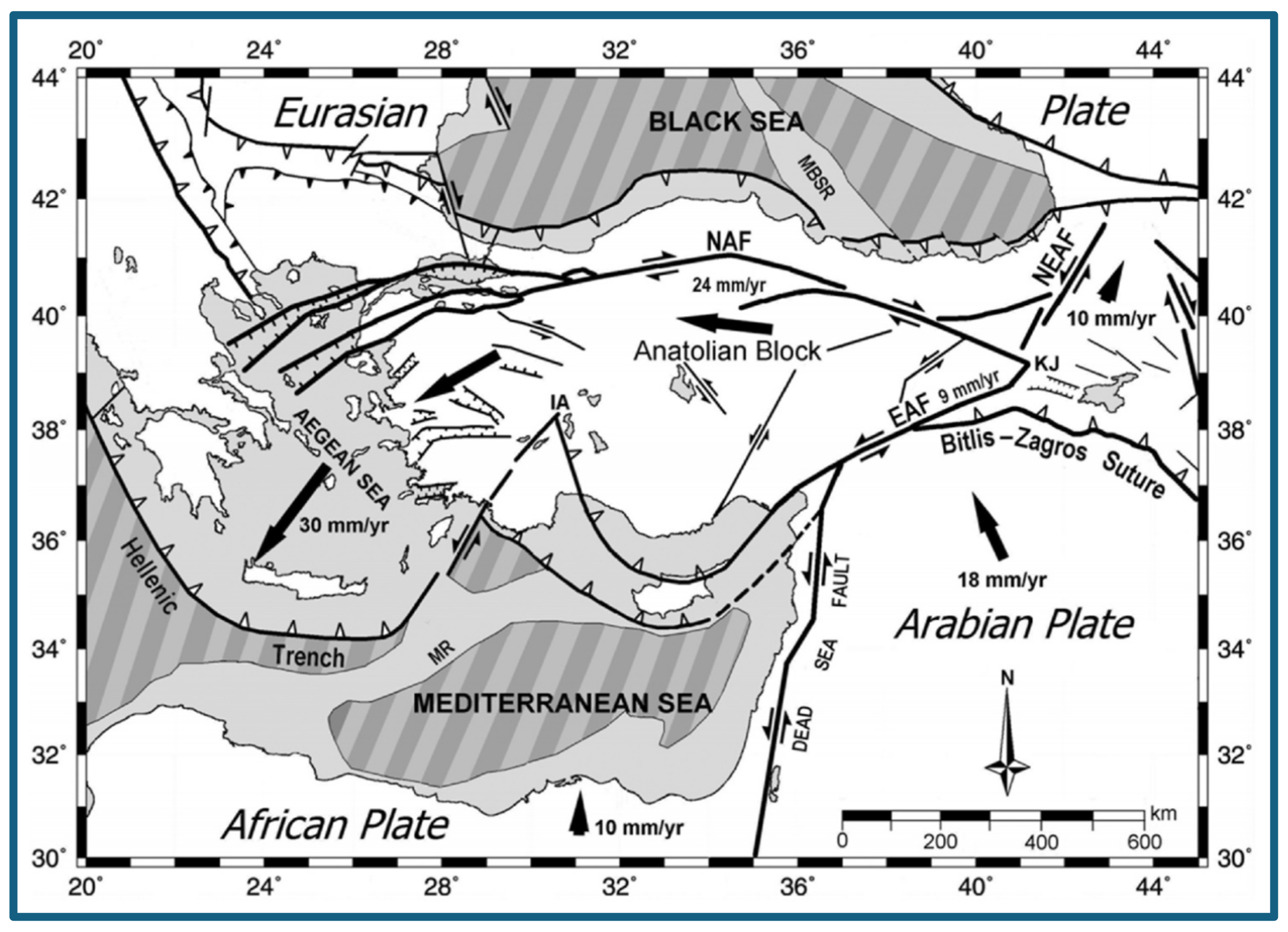
Türkiye is located in the Alpine–Himalayan mountain belt, which is known for its high level of tectonic activity. It lies on the boundaries of the Eurasian, African, and Arabian plates, making it one of the most geologically dynamic regions in the world [
1]. This region is characterized by active earthquake fault zones, including the North Anatolian Fault (NAF), East Anatolian Fault (EAF), and West Anatolian Fault (WAF) zones. These fault zones have the potential to generate destructive earthquakes, as evidenced by past events such as the 1999 Mw 7.6 Izmit, 1999 Mw 7.2 Düzce, 2011 Mw 7.1 Van, 2020 Mw 6.8 Elazıg, and 2020 Mw 7.0 Izmir earthquakes. The movement of the Arabian, Eurasian, and African plates, along with the Anatolian tectonic block, is primarily responsible for the significant seismic activity in Türkiye. The geological evolution of the area is a result of various significant interactions between major plate boundaries. These interactions involve subduction, extensive transform faulting, the formation of mountains through compression, and the extension of the Earth’s crust. The convergence of the African and Arabian plates with the Eurasian plate led to the closure of the Mediterranean Sea, resulting in the westward movement of the Anatolian block. This movement is predominantly accommodated along the North and East Anatolian faults. The convergence (subduction) boundary between the African plate in the south and the Anatolian block in the north is represented by the Cyprus Arc.
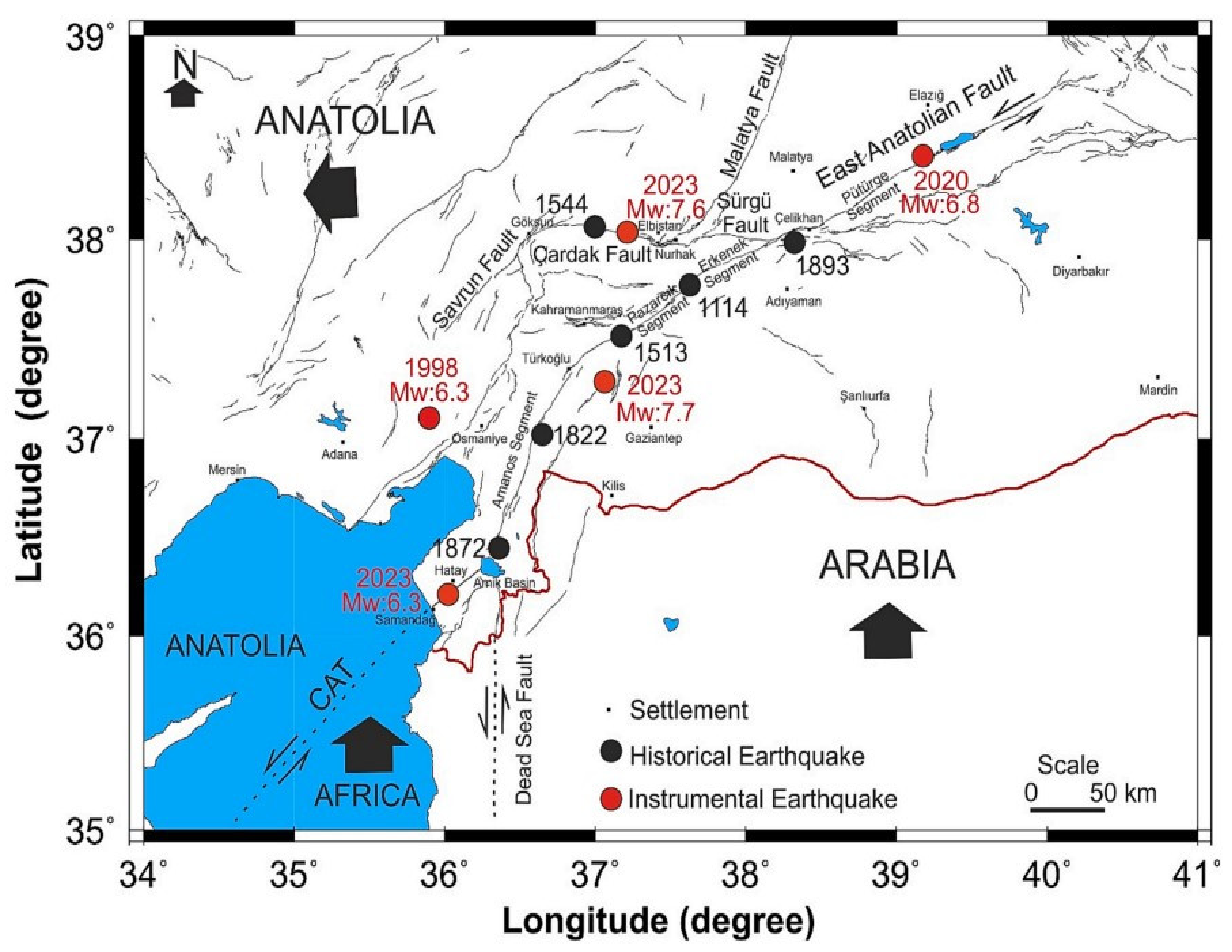
In 1999, Türkiye experienced one of its most catastrophic earthquakes in recent history, measuring 7.6 in magnitude near Izmit. This tragic event resulted in the loss of more than 16,900 lives and left a vast number of individuals without homes [
2]. However, the impact of the disaster reached new levels on 6 February 2023, when a seismic event of significant magnitude, measuring 7.7, struck near Pazarcik city in southern Turkey. This was followed by a second earthquake, measuring 7.5 magnitude, near Elbistan city 9 h later. The focal depths of these earthquakes were recorded at 8.6 km and 7.0 km, respectively. Fourteen days later, another significant earthquake with a magnitude of 6.4 occurred in Define, Hatay. The aftermath of these earthquakes was marked by over 11,000 aftershocks, as reported by Türkiye’s Disaster and Emergency Management Authority (AFAD). In total, more than 50,000 lives were lost, over 107,000 injuries were sustained, and extensive damage occurred across multiple provinces.
When such an event occurs, it is commonly assumed that neighboring regions experience an increase in stress. Over time, these stresses are relieved, resulting in aftershocks [
3,
4,
5,
6,
7,
8,
9]. The current study aims to provide detailed and precise statistical inferences regarding the sequence of aftershocks in Kahramanmaras. To achieve this, the statistical evolution of the aftershock data was analyzed, including parameters such as the
b-value, decay rate (
p-value), fractal dimension (
Dc-
value), and slip ratio. These analyses shed light on the seismotectonic properties of the area. Additionally, the changes in Coulomb stress resulting from the mainshock coseismic slip were evaluated to explain the occurrence of aftershocks. This study focuses on examining the geographic distribution of the Kahramanmaras sequence and sheds light on the underlying faults responsible for it. By analyzing this sequence, we can gain valuable knowledge about the local tectonic activity. It is crucial to uncover the geometry of the fault zone in order to comprehend the evolution of faults and the mechanics behind earthquake rupture. The findings of this research will contribute to the development of a comprehensive earthquake hazard model for the region.
Several studies, including [
10,
11,
12], have utilized global earthquake catalogs to gain insights into the complexity of earthquakes and to make predictions about their occurrence in terms of size, time, and location. Additionally, these studies have employed two robust empirical laws, namely the Gutenberg–Richter law and the Omori law, to characterize seismicity patterns. It has been observed that the productivity of aftershocks and the rate at which they decay are influenced by the faulting style of the mainshock. Specifically, strike-slip events exhibit a lower aftershock rate and a larger
p-value compared to thrust and normal events, respectively [
11]. In the studied region and its surroundings, the sinistral strike-slip mechanism of the East Anatolian Fault Zone (EAFZ) and Dead Sea Fault Zone (DSFZ)—along with the Cyprus Arc (CA) in southern Turkey, and the dextral strike-slip dominance along the North Anatolian Fault Zone (NAFZ) in the north—primarily accommodate the motion. This dynamic could potentially lead to an increased decay rate and a decrease in aftershock productivity [
13].
3. Data Collection, Methodology, and Data Analyses
The Incorporated Research Institutions for Seismology (IRIS) is a non-profit consortium consisting of more than 120 universities in the United States. Its primary focus is on the acquisition, management, and distribution of seismological data, while also fostering collaboration among researchers globally. IRIS is committed to advancing our understanding of the Earth through seismological research, education, and outreach. The organization strongly advocates for open access to seismic data and tools, ensuring that the global scientific community can benefit from them. IRIS operates multiple data centers that gather, store, and disseminate seismic data from various networks across the globe. These data centers offer real-time and historical seismic data, as well as analysis and visualization tools. With a network of over 150 stations, IRIS offers a comprehensive global span for studying seismic activities and structure of the Earth’s interior.
The earthquake data within a specified region, defined by latitudes 35.0°–39.0° N and longitudes 34.0°–41.0° E, has been compiled for the period between 6 February 2023 and 10 January 2024. This dataset consists of 471 local earthquakes, ranging in magnitude from 3.3 to 7.8, and focal depths vary between 0 to 27 km. To quantitatively analyze these data and the subsequent aftershock sequence, we have utilized two widely recognized scaling relationships in our study: the Gutenberg–Richter (G-R) frequency magnitude law [
27] and the Modified Omori’s Law/Omori–Utsu relationship [
28]. Statistical analyses of the dataset have been conducted using the ZMAP (version 6.0) software package [
29], a commercial software language which incorporates a range of tools written in Matlab
®. The software package comes with a graphical user interface (GUI), which offers various features such as catalog quality assessment (including artifact detection, and completeness evaluation), exploratory data analysis, identification of seismicity, and fractal dimension determination.
3.1. b-values and Magnitude of Completeness (Mc)
The earthquake frequency–magnitude distribution (FMD), commonly referred to as the Gutenberg–Richter relationship, is a commonly used power-law relation in seismicity studies. It was first introduced by [
30] and further developed by [
27]. This relationship establishes a correlation that links the frequency of earthquake occurrences with the distribution of magnitudes. This relationship is defined by Equation (1), which relates the cumulative seismic event count,
N(M), with magnitudes
M and higher.
The seismicity parameters constants, denoted as ‘
a’ and ‘
b’, play a crucial role in seismology. The parameter ‘
a’ represents the level of seismicity, while ‘
b’ signifies the slope of the FMD. In particular, the parameter ‘
b’ holds great importance in seismology due to its association with various geotectonic characteristics of a specific region [
31,
32]. Over the past several years, seismologists have extensively utilized the significance of ‘
b’ in earthquake prediction [
33,
34] and for quantifying seismicity [
35]. The
b-value has been found to vary significantly on a local scale, ranging from 0.3 to 2.5 [
36,
37,
38,
39,
40,
41,
42]. These variations can be attributed to various factors such as tectonic setting, focal depth, crustal heterogeneity, incomplete catalog data, predominant stress state, clustering of events, geothermal gradient, pore pressure, environmental or geophysical specifications, and method of calculation. All these elements, except for the method of calculation, are connected to the state of stress, either explicitly or implicitly [
43]. However, in most cases, the
b-value remains near one for extended durations and vast regions. In addition to indicating earthquake distribution, the
b-value also provides insights into the stress conditions of a region [
44].
It seems that an increase in the
b-value above 1.0 suggests regions with minimal exerted stress and crustal diversity, whereas values below 1.0 indicate significant unequal stress and uniformity of crust composition [
45,
46,
47]. Nevertheless, there are multiple approaches employed to compute the
b-value. In this study, we evaluated the
b-value using the Maximum Likelihood (ML) approach, which is implied in Equation (1). It is the most robust and widely acknowledged technique for calculating the
b-value, as proposed by Aki [
48] using the following formula:
where the minimum magnitude
represents the magnitude of completeness (
Mc) or the threshold magnitude for earthquakes, while the mean magnitude
and magnitude resolution
are also important factors. The
Mc plays a crucial role in seismicity research, serving as the minimum magnitude required for accurate reporting of earthquake magnitudes. Determining
Mc can be achieved by assuming the power-law distribution of G-R in relation to magnitude, as suggested by Wiemer and Wyss [
46].
The Frequency Magnitude Distribution (FMD) chart provides a visual representation of various aspects of the data and their analysis. In the FMD chart, a straight line is typically used to represent the best-fit line according to the Gutenberg–Richter frequency–magnitude relationship. Squares on the chart represent the actual observed data points for specific magnitude intervals, while triangles are often used to denote estimated cumulative frequencies or other derived data points. The slope of the straight line (the
b-
value) is critical for understanding the seismic characteristics of the region. A steeper slope indicates a higher frequency of smaller earthquakes relative to larger ones. Each square corresponds to a magnitude range and shows the number of earthquakes that occurred within that range during the observation period. The use of triangles to represent estimated cumulative frequencies allows researchers to visually assess the fit of the Gutenberg–Richter model across the entire magnitude range, especially in cases where data may be sparse or incomplete. This helps in identifying any discrepancies between observed data (squares) and model expectations (straight line). The distribution of the squares and triangles on the chart can also help in assessing the completeness of the seismic catalog and identifying any potential anomalies in the observed seismicity. Deviations from the straight line—such as a flattening of the curve at low magnitudes, indicated by the distribution of triangles and squares, may suggest issues with the magnitude of completeness (Mc) or a change in seismicity pattern, such as seismic quiescence or swarm-like behavior [
43,
44,
45,
46].
3.2. Decay Rate of Aftershocks (p-value)
It is widely acknowledged that the decline in aftershock activity over time (decay rate) is governed by the modified Omori law or Omori–Utsu law [
49]. This law provides a description of the anticipated number of aftershocks occurring at a specific time after a mainshock event.
where
shows the elapsed time since the mainshock. The constants
,
and
collectively define the shape and characteristics of the aftershock sequence.
, which is related to the overall productivity of aftershocks, provides valuable insights into the shape and intensity of the sequence. It is dependent on the total number of earthquakes in the sequence. On the other hand,
represents the rate of activity in the initial phase of the sequence. It also signifies the characteristic time scale over which aftershock activity decays. Smaller values of c indicate a more rapid decay of activity. Lastly,
is associated with the power law decay of aftershocks and influences the rate at which aftershock activity declines over time. A higher value of
suggests a slower decay rate, while a lower value indicates a faster decay. By adjusting the parameters
,
, and
, the particular seismic data can be tailored to suit a personalized model. Among these parameters,
holds the most significance and importance. Its range of variation is typically between 0.6 and 1.8, as observed in studies by [
45,
50]. It is worth noting that there may be variations of the Omori formula, and modifications can be made to account for different geological and seismological conditions. Furthermore, these parameters are often computed using statistical methods, such as Maximum Likelihood Estimation (MLE), based on observed seismic data.
The decay of aftershocks is believed to represent the rearrangement of stress caused by variations in stress resulting from the mainshock. The adjustment of stress can be seen as a reflection of the complex relaxation processes [
51], as well as the structural heterogeneity within the source volume [
49,
52] associated with the geological framework of the area. It remains uncertain which physical factors hold significance in determining the
p-value. The value of
p seems to be unaffected by the magnitude of completeness,
Mc. On the other hand, the
c-value is largely influenced by
Mc [
53]. It is probable that the absence of data right after the initial earthquake is the reason why numerous minor aftershocks cannot be identified on seismograph readings. The knowledge surrounding the chaotic characteristics of the
p-value in the crust is restricted. Various factors can be attributed to this phenomenon. For instance, [
54] suggested that
< 1 is commonly observed in aftershock series with normal mechanisms, whereas aftershocks that precede a large earthquake have
> 1. Significant attention is given to the determination of the
-
value using the ML technique, as recommended by [
55,
56].
3.3. Spatial Aftershock Distribution (Correlation Integral and Fractal Dimension)
Fractal properties can be observed in fault networks and epicenter distributions [
57,
58]. Consequently, the seismic activity distribution can be examined by calculating the fractal dimension, also referred to as the
Dc-
value. This fractal dimension extends beyond Euclidean dimensions and quantifies the level of earthquake clustering. The application of fractal dimensions allows for the examination of self-similarity in fault tectonics and seismicity phenomena and processes.
Fractal distributions are unique in that they lack a specific length scale and are therefore suitable for describing scale-invariant phenomena. In a two-dimensional space, the decimal value of
Dc can range from 0 to 2.0. When
Dc values tend towards 0, the events are increasingly distributed on a singular point. As
Dc approaches 1.0 in a space with 2-D, the event’s distributions become more linear. This same trend can be observed in the events’ distribution across a fracture. However, as
Dc tends towards 2.0, the events become evenly distributed throughout the plane [
59,
60]. The correlation dimension is utilized to compute the
Dc values, which are specified by [
46] as follows:
where the sphere radius being analyzed in the research is denoted as r, while the correlation integral is represented as C(r):
The quantity
N(
R <
r) represents the pairs count (
Xi,
Xj) that have a distance smaller than r. In the case of a fractal structure in the epicenter distribution, the subsequent correlation is derived:
The fractal dimension, denoted as
Dc, is specifically the correlation dimension [
61]. The estimation of the fractal dimension of the spatial distribution of earthquakes is achieved through the utilization of this relationship. By plotting
C(r) against r on a coordinate system with double logarithmic scales, the fractal dimension
Dc can be determined. The fractal dimension (
Dc) value is derived by drawing a blue tangent line to the fractal curve typically at a log–log scale. This line represents the linear correlation between the logarithm of the number of boxes and the logarithm of the box size. The slope (gradient) of this tangent line indicates the fractal dimension. The distance r between two events, (
Θ1,
Φ1) and (
Θ2,
Φ2), is measured by using a spherical triangle as described by Hirata [
62]:
where
and
represent, respectively, the geographic coordinates (latitudes and longitudes) of the ith and jth events. A least-square line is fitted in the scaling region to obtain the slope.
3.4. Slip Ratio (SP/S)
The slip, which refers to the relative displacement of points that were once adjacent on opposite sides of a fault, is a significant mechanism of crustal deformation. Typically, a portion of the slip takes place on the primary fault system, leading to the occurrence of the largest (and smallest) earthquakes, while the remaining slip occurs on the secondary fault segment [
63]. The slip ratio, which represents the proportion of slip occurring on the primary fault compared to the total slip, can be determined by evaluating the spatial fractal dimension as:
where the slip atop the principal fault (
) and the cumulative slip along the fault system (
), are two distinct measurements used to quantify the displacement along the fault [
63,
64]. When
Dc equals 3, the complete slip rate is diverted towards the secondary faults, which are smaller in size. Conversely, when
Dc is equal to 0, the entire slip is discharged on the principal fault.
The flowchart shown in
Figure 4 illustrates the interconnections among the
b-value,
p-value, fractal dimension, and slip ratio. These relationships provide valuable insights into the seismicity, fault behavior, and earthquake hazard of the studied region. However, the precise nature of these relationships may differ based on the geological context and the specific characteristics of the seismic data under analysis.
3.5. Coseismic Coulomb Stress Changes
Coulomb stress pertains to the shear stress exerted on a fault or rock mass due to tectonic forces. It quantifies the additional stress that can either facilitate or impede fault movement, depending on whether it aligns with or opposes the existing stress on the fault plane. In the fields of geology and seismology, Coulomb stress is utilized to evaluate the probability of earthquake occurrence and comprehend faulting mechanics. When the Coulomb stress surpasses a specific threshold, it has the potential to initiate or hinder fault movement, potentially resulting in earthquakes or aseismic slip. This concept is crucial for comprehending fault behavior mechanics and assessing seismic hazards. In certain instances, an escalation in Coulomb stress may encourage fault slip, leading to larger coseismic displacements; while in other cases, it may impede fault slip, resulting in smaller displacements. Coseismic displacement denotes the movement or displacement that transpires along a fault during an earthquake, specifically during the earthquake’s rupture period. It represents the instantaneous movement of rock masses on either side of a fault plane as a consequence of the accumulated strain being released during the seismic event. Alterations in Coulomb stress can influence the likelihood of fault slip and the magnitude of displacement during an earthquake. Moreover, the correlation between coseismic Coulomb stress and coseismic displacement can vary depending on factors such as the fault’s geometry and orientation, the regional stress field, and the mechanical properties of the rocks surrounding the fault [
65].
3.6. The Akaike Information Criterion (AIC): Description and Algorithm Validation
The Akaike Information Criterion (
AIC) is derived from information theory and serves as a means to estimate the amount of information that would be sacrificed if a specific model were employed to describe the underlying process of the analyzed data [
66]. By using AIC, one can compare and rank a collection of statistical models based on the extent of information loss in the investigated process. It is crucial to emphasize that
AIC is solely applicable for comparative purposes and cannot determine the absolute quality of a model. The formula for
AIC is expressed as follows:
The variable represents the quantity of data points, denotes the cumulative sum of squared residuals for the assessed model, and signifies the count of independent parameters within the model. According to Equation (9), the optimal model is estimated by the minimum value of that corresponds to the lowest value. Therefore, this model best represents the investigated process. For example, when comparing two potential models, their relative quality can be assessed by calculating the difference in values. This approach can also be used in reverse, such as in the context of seeking a particular action within a time series. In such a scenario, two models are selected: one that precisely characterizes the desired conduct and another that represents a different behavior.
The forecast aftershock occurrences using Maximum Likelihood Estimation (MLE) and Root Mean Square (RMS) analysis involves several key parameters that are vital for understanding and forecasting seismic aftershock sequences. These parameters include Omori parameters (p-value, c-value, and k-value), and power-law decay parameters (pm, cm, and km), which control the initial level, decay rate, and time scale of aftershock activity, respectively. The parameter pm signifies the rate of aftershock occurrence immediately following the mainshock, with a higher value indicating a greater initial level of activity. Conversely, cm determines the speed at which aftershock rates decrease post-mainshock, where a higher cm value denotes a slower decay, indicating prolonged aftershock activity. The parameter km reflects the time frame over which aftershock rates decrease, with higher values suggesting a longer-lasting aftershock period. Additionally, statistical measures such as the Kolmogorov–Smirnov (KS) test, Hurst exponent (H), KS statistic, and Root Mean Square (RMS) error are essential in assessing model fit and accuracy. The KS test evaluates how well predicted aftershock rates align with observed data, with a lower KS statistic indicating better agreement. The Hurst exponent quantifies long-term memory in aftershock occurrence patterns, with higher values indicating stronger persistence. The RMS error measures differences between predicted and observed values, with lower values signifying better predictive accuracy. Furthermore, parameters such as Effective Parameter Count (Epl) and Best Model (Bst) help assess model complexity and identify the most suitable model. Higher standard deviations (σ) associated with Epl and Bst indicate greater uncertainty in determining model complexity and selecting the best-fitting model, respectively. Overall, these parameters collectively contribute to a comprehensive understanding of aftershock behavior and aid in improving forecasting accuracy, while accounting for model uncertainty.
4. Results and Discussions
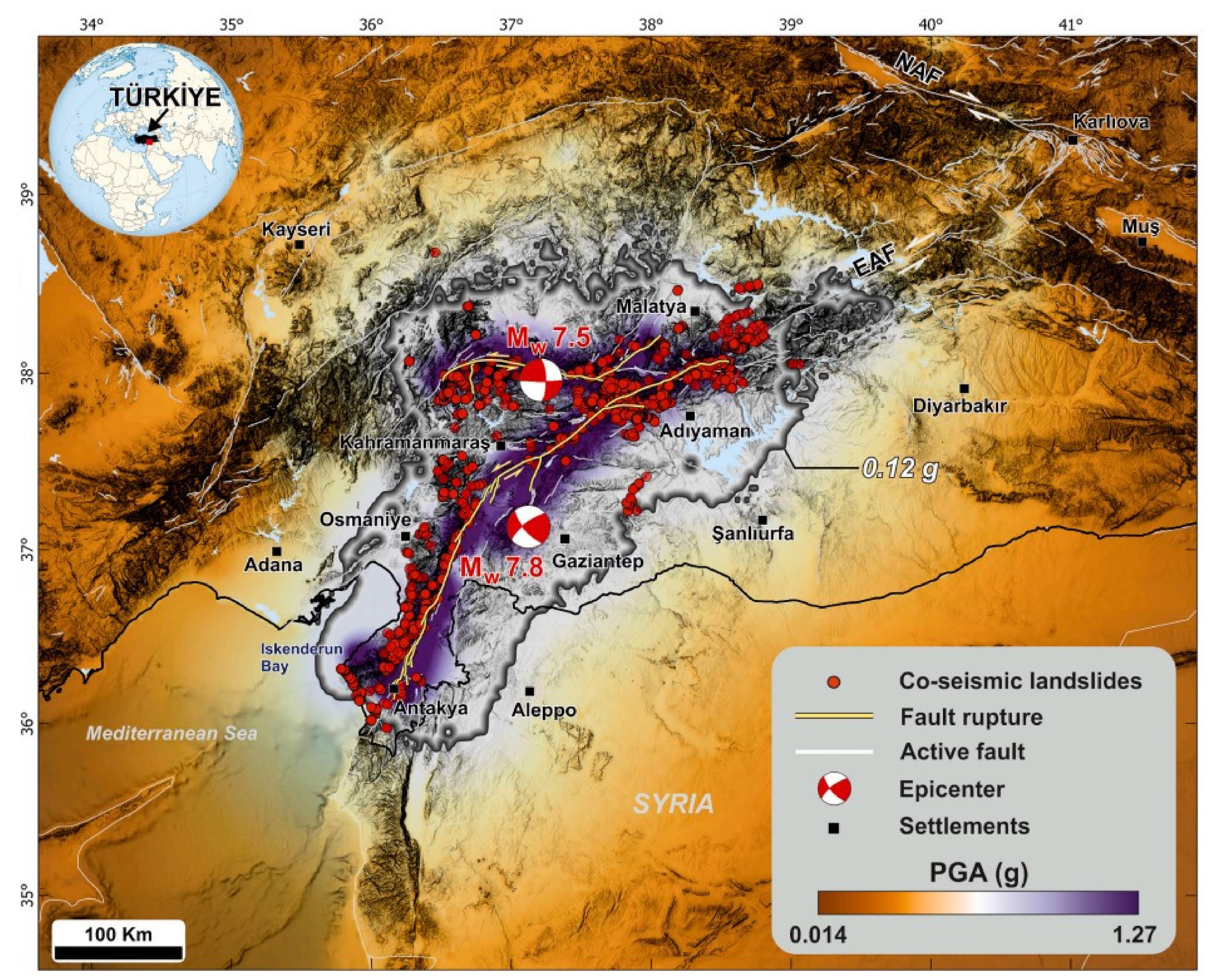
A series of powerful aftershocks (reaching up to Mw 6.7) have been observed subsequent to the occurrence of two consecutive earthquakes measuring Mw 7.8 and 7.5 (on 6 February 2023) along the segments of the East Anatolian Fault Zone (EAFZ). The estimation of the earthquake distribution using the
b-value and the decay rate of aftershocks (
p-value) has been conducted using the magnitude–frequency relation of Gutenberg and Richter (Equation (1)) and the modified Omori law (Equation (3)), respectively. In order to obtain accurate
b-value, events with a magnitude greater than the completeness magnitude (
Mc) were selected using the maximum curvature method.
Mc holds significant importance in seismicity-based research as it allows for the analysis of a maximum count of events with high quality. For the entire sequence, the
Mc of 4.4 was determined (
Figure 5), resulting in a calculated
b-value of 1.21 ± 0.03. The squares and triangles on the frequency–magnitude distribution plot often represent observed and estimated cumulative earthquakes for each magnitude value, respectively, which provide insights into the observed and predicted patterns of seismicity in the studied region (
Figure 5). Xu et al. [
67] conducted a study in the studied area to analyze the seismicity rates of events ranging from Mw 1–7 using the Gutenberg–Richter (G-R) law. Considering this, Melger et al. [
68] explored two different scenarios. The first scenario involved investigating the seismicity rates since a major earthquake was historically reported in 1114 (Mw = 7.8) up until 2022, with
b-values ranging approximately from 0.92 to 0.94. The second scenario focused on the period between 2007 and 2019, with
b-values of 1.1. In our study, the
b-value slightly surpasses those observed in the two scenarios mentioned and the global average of 1.0. This suggests that the Türkiye sequence is predominantly characterized by aftershocks with smaller magnitudes relative to larger ones, playing a role in regulating fluctuating crustal stress levels within the region, which reflects a more stable or less stressed seismic environment, where smaller earthquakes are more prevalent [
45,
46].
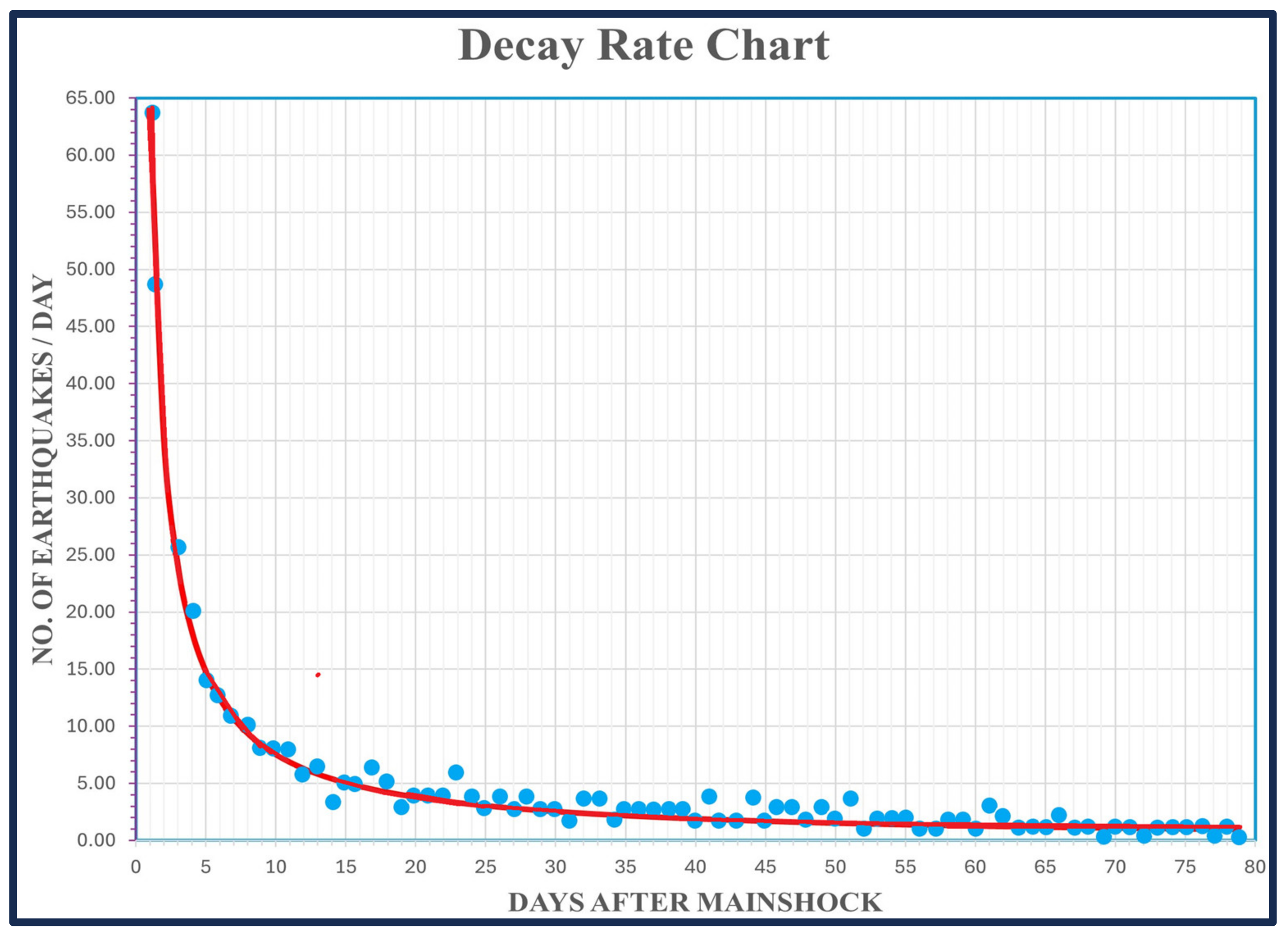
Figure 6 illustrates the rate at which aftershocks occurred within 80 days of the Türkiye earthquake doublet. The graph shows that the occurrence rate decreased rapidly from ~65 events per day immediately after the main shock, to ~15 events per day after the first 5 days, and then to about five events per day after 15 days. The rate then gradually declined over the course of 80 days. The decay characteristics of the Türkiye aftershock sequence were analyzed using the
p-value of the modified Omori law, as shown in
Figure 7. The parameters of Omori’s law primarily vary depending on the tectonic environment, such as the styles of faulting, in the region [
11]. The observed
p-value was found to be as low as 1.1 ± 0.04, which is slightly higher than the mean value of 1.0. A higher
p-value indicates a faster decay of aftershock activity. The characteristic time scale, represented by the
c-value, for the decay of aftershock activity was determined to be 0.204 ± 0.058. This suggests a relatively moderate or low initial productivity of aftershocks. The point at which the observed rate of aftershocks starts to follow the predicted decay pattern is known as the “decaying onset”. This point typically aligns closely with the parameter
c, which helps adjust the model to match the start of the decay curve. By visually examining the graph representing the decay curve and identifying the c value (
Figure 7), we can observe the moment when the curve starts to sharply decline from its peak. This adjusted point, determined by the
c value, offers an estimate of when the decay rate begins to significantly decrease, indicating the onset of decay. The
c parameter itself provides a quantitative estimate of this onset, representing the time offset from t = 0 (the time of the mainshock) where the Omori–Utsu formula becomes a suitable fit for the data. Therefore, the value of
c, expressed in the same time units as the
x-axis of the graph (usually days), can be understood as the estimated day of the decaying onset following the mainshock. The constant (
k-value) in the Omori formula, which is related to the overall productivity of aftershocks, was calculated to be 76.75 ± 8.84. This suggests that the decrease in aftershock activity began between approximately 68 to 86 after the occurrence of the mainshocks, as shown in
Figure 7. By comparing this outcome with
Figure 6, we can infer that the decay in aftershock activity commenced 68 days following the mainshocks’ occurrence.
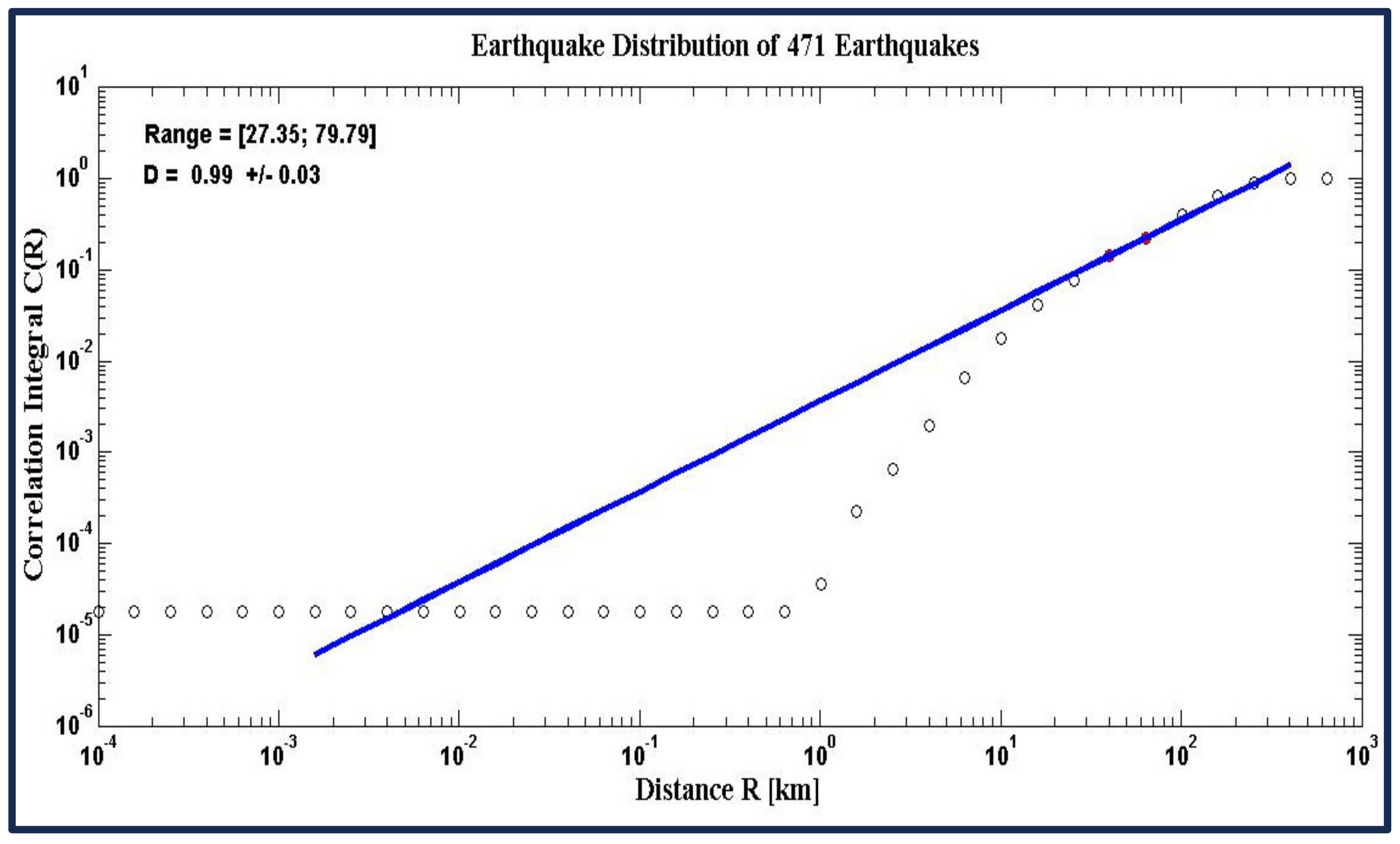
Bayrak and Kirci [
69] conducted an analysis of active fault data along the East Anatolian Fault Zone (EAFZ) using both manual (classic) and modern versions of the box counting method. The fractal analysis revealed that the total fault length along the EAFZ is 450 km (15 × 30 km), with a fault area of 13,500 km
2. The fractal dimensions of the main EAFZ fault trace, calculated using the manual box counting method, ranged from 0.81 to 1.47. The highest fractal dimension value (1.47) was observed in the Karlıova region and its surroundings, while the lowest value (0.81) was found in the area around Hazar Lake. The fractal dimension values for the areas surrounding the two main shocks, were 1.15 and 1.21 (determined using the manual box counting method) and 1.01 and 1.13 (determined using the Free box and Grid methods), respectively. In contrast, Sarp [
70] utilized the box-counting method to determine the fractal dimension of major fault networks along the EAFZ, resulting in values ranging from 0.90 to 1.23. In this study, the determination of the fractal dimension (
Dc) involved analyzing the characteristics of earthquake sites, including epicenters and hypocenters. To calculate the fractal dimension, the box-counting technique was utilized. The research area was partitioned into a series of smaller boxes, and the count of boxes with at least one earthquake was documented for different box dimensions. A linear relationship can be observed by graphing the quantity of boxes against the size of the box (both in a logarithmic scale). The data points corresponding to the chosen earthquakes on the fractal curve were determined, and logarithmic transformations were applied to them. The slope of the tangent line was then calculated using linear regression analysis. Following that, a blue tangent line was usually drawn on the fractal curve at a logarithmic scale. The slope of this line represents the fractal dimension. In the case of the Türkiye sequence, the fractal dimension (
Figure 8) was determined to be 0.99 ± 0.03 by analyzing the correlation integral and distance between hypocenters using data from 471 earthquakes. Despite considering the three-dimensional space, the fractal dimension value being smaller than 1.0 suggests that the events are clustered and distributed along the fault line. Xu et al. [
67] indicated that the long-term slip rates inferred from GPS data prior to the latest significant earthquakes range from 3 to 7 mm/year. From the east to the west along the East Anatolian Fault (EAF), the slip rates substantially decrease to 1–4 mm/year. The slip ratio that arises from the sequence of aftershocks pertains to the proportion of the overall fault slip that occurred during the seismic event, in relation to the total length of the fault rupture. This ratio quantifies the extent of fault slip relative to the length of the fault that was involved in the earthquake. In the case of the Türkiye sequence, where
Dc = 0.99, the slip ratio is determined to be 0.75. In simpler terms, 75% of the total slip is attributed to the primary rupture during the Türkiye sequence, while the remaining 25% is distributed across the secondary rupture. Melgar et al. [
68] demonstrated that the EAF exhibits a maximum slip of 8 m, primarily concentrated at depths ranging from 3 to 7 km, indicating a shallow slip deficit. Similarly, the Çardak fault experiences a maximum slip of 11 m during the Mw 7.6 aftershock, extending from the surface to a depth of 7 km.
The initial phase of the M 7.8 earthquake caused a rupture in a fault segment that spans approximately 50 km to the east of the main East Anatolian fault (EAF). This segment is located along the northern extension of the Dead Sea fault (DSF) in the southern region. The Coulomb stress changes resulting from this initial rupture indicate positive values to the northeast of the EAF, suggesting that this initial slip may have played a role in triggering slip on the EAF. The complete rupture of the Mw 7.8 earthquake, as observed through remote sensing, covered a section of the EAF that spans approximately 300 km. The resulting Coulomb stress changes on the Sürgü fault, which is an east-west trending fault in the area where the Mw 7.5 aftershock originated, also show positive values. This indicates that the M 7.8 event may have contributed to triggering the Mw 7.5 earthquake that occurred about 9 h later. Lastly, the Coulomb stress change modelling can be used to evaluate how the overall sequence of earthquakes, including the Mw 7.8 and Mw 7.5 events, has altered the regional stress state.
Figure 9a illustrates the Coulomb stress change on left-lateral strike-slip faults that strike in a northward direction, similar to the DSF. The northern part of the DSF, just south of the Mw 7.8 epicenter, as well as the western end of the Sürgü fault, have been loaded.
Figure 9b displays the Coulomb stress change on left-lateral strike-slip faults that strike in a northeastward direction, like the EAF. The majority of the EAF has been relieved of stress due to the mainshock slip on this structure, although there are still areas of stress increase at the ends of the rupture on the EAF [
65].
The Akaike Information Criterion (
AIC) is a useful tool in aftershock modelling for comparing the fit of different models, such as the Maximum Likelihood Estimation (MLE) and the Root Mean Square (RMS) models, to observed aftershock data (
Figure 10). Models with lower
AIC values are better fitting, indicating that they provide a more accurate representation of the observed data. Aftershock modelling fit refers to how well a specific aftershock model, such as MLE or RMS, captures the observed patterns and behaviors of aftershocks following a mainshock. By comparing the predictions of these models to observed aftershock data, the
AIC can be used as a quantitative measure to evaluate their fit. A lower
AIC value suggests a better fit, indicating that the model provides a more accurate representation of the observed aftershock sequence. The Maximum Likelihood Estimation (MLE) is a statistical method utilized to estimate the parameters of a probability distribution that most accurately represents the observed data. In the context of aftershock activity, the MLE model is employed to estimate parameters such as the decay rate. On the other hand, the Root Mean Square (RMS) model is a physical model that describes the behavior of faults and the generation of earthquakes by considering frictional properties. The dashed vertical line at time = 20 days in
Figure 10 represents the minimum
AIC value or the
AIC value of the best-performing model among those under comparison. Essentially, it signifies the model that offers the optimal trade-off between goodness of fit and complexity, as per the
AIC criterion.
By utilizing the RMS model, it becomes possible to simulate the occurrence and behavior of aftershocks based on the fault’s frictional characteristics. By analyzing the
AIC, the optimal model that provides the best fit can be selected. In the case of forecasting aftershock occurrence using the MLE model, the following results are obtained: The Omori parameters indicate a decay rate of (
p = 1.25,
c = 0.25, and
k = 88.2). Additionally, a modified version of the Omori formula incorporates a power-law decay parameter, which shows values of (
pm = 1.09,
cm = 0.163, and
km = 72.5). Furthermore, the Kolmogorov–Smirnov (
KS) test is utilized to compare the observed data distribution with the expected distribution from the model, and supplementary statistics are also provided (
Figure 11). The data presented include the null hypothesis (
H = 0), with a
KS statistic of 0.064 and a
p-value of 0.499. A higher
p-value suggests that the model is a good fit for the data. The Root Mean Square (
RMS = 8.427) measures the average difference between observed and predicted values. Lower
RMS values indicate a better fit. The standard deviation of the best-fit model,
σ(Bst), is 31.04. The seismicity rate change parameter,
Rc, is 0.08. The
AIC is used for model selection, where models with reduced
AIC values suggest a more optimal trade-off between accuracy and complexity (
AIC = −1788.73). The forecasted aftershock occurrence using the RMS model yields the following results: The Omori parameters are (
p = 1.08,
c = 0.19, and
k = 75.2). The standard deviations of the best-fit model for aftershock occurrence are
σ(Epl) = 59.4 and
σ(Bst) = 34.6. A lower value indicates a better fit to the observed data. The parameters associated with seismicity rate changes are
Rc(Epl) = −0.149 and
Rc(Bst) = −0.256. These parameters provide insights into the expected modifications in seismic activity, capturing the influence of the aftershock sequence on the overall seismicity rate. The evaluation of different models in representing the decline of aftershock rate over time has been evaluated, and the most optimal model is illustrated in
Figure 11 and
Table 1.
5. Conclusions
The present study examines the occurrence of earthquakes during the Türkiye sequence through the use of statistical models and coseismic Coulomb stress modelling. To accomplish this objective, several parameters including b-value, p-value, Dc-value, slip ratio, and coulomb stress transfer were calculated. The estimated b-value is 1.21 ± 0.1, indicating that the East Anatolian Fault Zone (EAFZ) exhibits complex stress distribution patterns and frequent seismic activity characterized by larger magnitude aftershocks. This elevated b-value could be indicative of heterogeneity in the fault zone, potentially caused by the presence of fault asperities or variations in the crustal composition that impact stress accumulation and release mechanisms. The aftershock decay rate (p-value = 1.1 ± 0.04) indicates that the frequency of aftershocks decreases linearly with time. In the context of the EAFZ, this implies a persistent release of stress post-mainshock, which is typical for fault zones with significant stored elastic energy and ongoing tectonic deformation. Meanwhile, the observed moderate c-value of 0.204 ± 0.058 suggests a delay in the initiation of the aftershock sequence, possibly due to the complex rupture dynamics or the presence of barriers to rupture propagation within the fault zone. Additionally, the k-value of 76.75 ± 8.84 indicates a substantial amount of aftershock activity, pointing to the release of a significant amount of accumulated stress over a relatively extended period following the mainshocks occurred, which nearly disappeared approximately 68 to 86 days after the occurrence of the main shocks. By referring to the decay rate chart we can infer that the decay in aftershock activity commenced 68 days following the mainshocks’ occurrence. The fractal dimension Dc, determined using integral correlation, has been utilized to assess the slip ratio on the primary fault segment. The fractal dimension (Dc) of 0.99 ± 0.03 suggests that aftershock activity is highly localized along the main fault trace or closely parallel subsidiary structures. This linear clustering is indicative of a distinct, dominant fault structure that significantly influences seismicity patterns. Analysis of the slip ratio during the aftershock activity reveals that 75% of the total slip occurred in the primary rupture, while the remaining portion was distributed across secondary faults, indicating that the aftershocks occurred on slightly fractured rock mass. This distribution could imply that a significant amount of strain along the fault was released during the mainshock, with the remaining 25% accommodated through aftershock activity and potentially aseismic slip. This high slip ratio could point to a highly dynamic rupture process during the mainshock, with significant implications for understanding the seismic hazard posed by future large events on the EAFZ. The earthquake sequence likely induced stress changes in the region’s crust, potentially triggering or facilitating further rupture on neighboring faults. For instance, the Sürgü fault experienced the Mw 7.5 earthquake and significant aftershock activity. In sum, these parameters reveal a fault system characterized by complex stress distribution, significant heterogeneity, and a tendency to release accumulated tectonic stress through both seismic and aseismic mechanisms. The data suggest that the EAFZ is an active tectonic feature capable of generating large earthquakes and a complex aftershock sequence. This analysis can enhance seismic hazard assessment models for the region, particularly in predicting the distribution and magnitude of aftershocks following major seismic events. Moreover, understanding these dynamics can assist in preparing for future seismic activity through improved building codes, urban planning, and emergency response strategies.
In conclusion, this study has provided valuable insights into the underlying mechanisms of aftershock occurrences following recent major earthquakes in Türkiye. It has uncovered significant findings, including the rapid decrease in stress levels post-main shocks and the tendency towards clustering in aftershock seismicity. These findings challenge existing theories and contribute to a deeper understanding of earthquake dynamics. Our research has also addressed gaps in the current understanding of aftershock sequences in complex fault zones and demonstrated how it can be applied to improve predictive models for earthquake aftershock sequences globally. Additionally, by comparing our findings with existing literature, we have highlighted variations in aftershock characteristics, deepening our understanding of seismic activity variability and providing valuable insights for future research endeavors. While this study focused on specific seismic events and models, the methodologies and insights gained can be extrapolated to assist in forecasting aftershock occurrences for future earthquakes. By refining our understanding of aftershock dynamics and enhancing the accuracy of forecasting models, we can establish a solid foundation for more effective strategies in assessing seismic hazards and managing disaster risks.


