Article

Analyzing the Influence of Dean Number on an Accelerated Toroidal: Insights from Particle Imaging Velocimetry Gyroscope (PIVG)

1
Department of Mechanical and Manufacturing Engineering, Schulich School of Engineering, University of Calgary, 2500 University Dr. NW, Calgary, AB T2N 1N4, Canada
2
Department of Geomatics Engineering, Schulich School of Engineering, University of Calgary, 2500 University Dr. NW, Calgary, AB T2N 1N4, Canada
*
Author to whom correspondence should be addressed.
Submission received: 18 March 2024 / Revised: 14 April 2024 / Accepted: 22 April 2024 / Published: 25 April 2024
(This article belongs to the Special Issue Flow Visualization: Experiments and Techniques)

Abstract

:
Computational Fluid Dynamics (CFD) simulations were utilized in this study to comprehensively explore the fluid dynamics within an accelerated toroidal vessel, specifically those central to Particle Imaging Velocimetry Gyroscope (PIVG) technology. To ensure the robustness of our simulations, we systematically conducted grid convergence studies and quantified uncertainties, affirming the stability, accuracy, and reliability of our computational grid and results. Comprehensive validation against experimental data further confirmed our simulations’ fidelity, emphasizing the model’s fidelity. As the PIVG is set up to address the primary flow through the toroidal pipe, we focused on the interaction between the primary and secondary flows to provide insights into the relevant dynamics of the fluid. In our investigation covering Dean numbers (De) from 10 to 70, we analyzed diverse aspects, including primary flow, secondary flow patterns, pressure distribution, and the interrelation between primary and secondary flows within toroidal structures, offering a comprehensive view across this range. Our research indicated stability and fully developed fluid dynamics within the toroidal pipe under accelerated angular velocity, particularly for low De. Furthermore, we identified an optimal Dean number of 11, which corresponded to ideal dimensions for the toroidal geometry with a curvature radius of 25 mm and a cross-sectional diameter of 5 mm. This study enhances our understanding of toroidal fluid dynamics and highlights the pivotal role of CFD in optimizing toroidal vessel design for advanced navigation technologies.

1. Introduction

Inertial measurement units (IMUs) are integral components of navigation systems; they provide essential information about a moving platform’s position, velocity, and attitude. IMUs rely on the accurate measurement of linear acceleration and angular rate. However, the traditional gyroscopes used in commercial IMUs suffer from bias instability, which affects their performance and introduces errors in attitude estimation. To overcome this limitation, novel gyroscope technologies are being explored to improve the accuracy and reliability of IMUs [1,2,3].
One such emerging technology is the Particle Imaging Velocimetry Gyroscope (PIVG). The PIVG is a fluid-based gyroscope that offers several advantages over conventional gyroscopes. It is nearly drift-free and exhibits minimal bias instability, even for navigation-grade IMUs. Additionally, the PIVG boasts a high signal-to-noise ratio (SNR), making it an attractive alternative for various navigation applications. Moreover, its low cost makes it a cost-effective solution in comparison to traditional gyroscopes. The PIVGs are constructed with three channels that are arranged in perpendicular axes, each with a circular, toroidal shape. A significant process employed in this configuration is Particle Imaging Velocimetry (PIV). This involves utilizing digital cameras to capture images of particles while they move through the water within toroidal channels. After capture, the images undergo processing; determining the displacement of each particle provides a measurement indicating fluid velocity. This information allows us to calculate the angular acceleration of the toroidal structure and provides valuable insights into the rotational dynamics of the PIVG. This three-axis design allows the gyroscope to comprehensively measure angular motion in multiple dimensions. However, for some applications, the design can be simplified to a single-axis system by using only one circular channel, making the construction more streamlined and less complex [1].
The study of fluid flow behavior in curved geometries is significant in various engineering applications, such as pipeline systems, ducting in internal combustion engines, heat exchangers, biological system flows, and microfluidic devices [4]. This behavior, which is complex in nature, exhibits secondary flows and vortices. Our literature review focuses on two phenomena: pressure-driven flow and rotating or spinning curved pipes. By leveraging insights from these studies, we can enhance our understanding of the intricate fluid behavior within the toroidal chamber of the PIVG. These phenomena, despite their different driving mechanisms, share common dynamics and characteristics, underscoring the importance of their study in the context of fluid flow in curved structures.
In pressure-driven research, Dean proposed an analytical solution for Newtonian flow in a curved conduit with a circular cross-section in 1928 [5,6]. He considered the secondary flow as a minor perturbation upon the primary flow, like Poiseuille flows in a straight pipe. Dean’s study established that the axial velocity within a curved pipe and the stream function of the secondary radial flow depend on the curvature parameter (k), which is summarized in the equation:
k = 2 R e 2 a R
where “a” is the channel’s radius, “R” is the torus’s radius, and “Re” is the Reynolds number. Subsequently, White introduced the term “Dean’s number (De)”:
D e = R e a R
The Dean number (De) and the curvature number (k) provide valuable insights into the flow behavior in curved pipes. The Dean number measures the relative influence of centrifugal forces compared to viscous forces, indicating the fluid flow’s behavior. Simultaneously, the curvature number quantifies the importance of the pipe’s curvature in relation to the fluid’s viscosity. A crucial finding emerged in the insightful studies conducted by Ligrani [7] under laminar flow conditions. It was revealed that a critical limit exists for the Dean number, specifically in the De ≤ 40~60 range, under which the influence of secondary flows on the primary flow remains minimal. This vital understanding emphasizes the critical balance necessary to maintain the stability and integrity of the fluid dynamics within the given parameters.
On the other hand, in 1963 Greenspan and Howard [8], who were researching spinning curved pipes, employed linear techniques to investigate spin-up phenomena. They recognized three unique phases: the formation of Ekman boundary layers, secondary flow within the body of the fluid, and viscous decay of residual motion. Additionally, they applied linear theory to estimate the characteristic spin-up time for two cylindrical geometries. In the first scenario, the cylinder was bounded by a flat disk, while in the second, it was enclosed by a conical section. Notably, the disk and the conical sections rotated along the cylinder walls. Through experimentation, Greenspan and Howard validated their theoretical predictions in each case. Greenspan (1968) [9] provided specifics of the methods involved, and a significant portion of the early work in this field is described.
Moreover, Cowley et al. [10] studied the fluid inside a curved pipe rotated around its curvature axis. In the limit of a high De, they demonstrated that boundary-layer collision and unsteady separation can occur impulsively and can begin to flow through a stationary curved conduit. A more thorough explanation of this phenomenon is given by Lam [11], who also includes estimates of the flow caused by the impulsive rotation of a curved pipe around its curvature axis.
The work that aligns most closely with our research, albeit with different objectives, is the study conducted by Madden and Mullin in 1994 [12]. They explored how fluid flow behaved within a toroidal sealed pipe under the impact of inertial angular rotation. Their study aimed to examine fluid velocity affected by inertia and the effects of ocean flow on the earth’s surface. They performed experiments on a toroidal pipe filled with water. However, Laser Doppler Velocimetry (LDV) was used to track the fluid movement inside the toroidal pipe. Therefore, tracer particles were added to the stream. The tracer particles were observed to calculate the fluid flow velocity field in a Eulerian frame. Additionally, the study made sure that the toroidal pipe was not subjected to any external forces aside from the inertial force that was created when the pipe was spun about its vertical axis from rest up to a constant angular velocity with a linear acceleration ramp, ensuring the pipe reached its top speed in 0.8 s. The experimental setup measured the absolute velocity field in relation to a stationary LDV setup. Moreover, the study conducted a numerical simulation for various fluid flow channel dimensions to produce a definite conclusion regarding the fluid behavior under the effect of an angular rotation in the form of a spin-up from rest up to a specific angular velocity. However, the study’s computational and experimental results showed that the fluid flow inside the toroidal pipe would have two main components to its velocity. A primary flow constitutes the majority of the fluid flow and moves in the opposite direction of the pipe flow. A second fluid flow also exists, and it moves in the radial direction of the toroidal pipe cross-section.
In this study, our aim is to conduct a thorough investigation of the fluid dynamics within accelerated toroidal geometry and its implications for PIVG systems. Two key criteria were evaluated with Computational Fluid Dynamics (CFD), namely domain validity and model fidelity. The range of Dean numbers (De) for reliable predictions of fluid velocities within the profile, known as domain validity, and model fidelity, which evaluates the mathematical model’s accuracy in estimating these numbers needs to be considered when evaluating PIVG performance. Therefore, precise measurements of primary flow dynamics by integrated cameras are crucial for accurate angular acceleration measurement, which could be impeded by secondary flow phenomena. Hence, we examined primary and secondary flows across different toroidal channel dimensions and De ranges, and we analyzed pressure distributions during this study. According to empirical evidence, the Reynolds number is a key parameter, and laminar flow should not exceed 200, according to a literature review. Similarly, the Dean number plays a part in characterizing secondary flow effects; thus, a suggested range of 40–60 has been identified to reduce these effects while maintaining mostly one-dimensional profiles. Altogether, these criteria furnish a comprehensive framework for optimizing fluid dynamics within the PIVG, thereby ensuring its accurate operation and performance [1,2,13].
The structure of this paper is organized as follows. In Section 2, we present an overview of the governing equations that describe the fluid dynamics inside the toroidal geometry of the PIVG system. Section 3 presents our numerical setup for simulating fluid dynamics in the toroidal geometry, detailing the computational domain, boundary conditions, and solution methods for the governing equations. In Section 4, we ensure accuracy through grid convergence and validate our simulations against experiments, establishing credibility. We then present vital insights from our numerical analysis, following a systematic approach. Finally, in Section 5, we conclude the paper by summarizing the contributions of this study and highlighting the implications for the design and optimization of the toroidal geometry in fluid-based gyroscopes.

2. Governing Equations

In the study of fluid flow in toroidal pipes, a toroidal coordinate system (r, θ, ϕ), as shown in Figure 1, is commonly used. Here, ‘r’ is the coordinate along the radial direction, ‘θ’ represents the inclination of the cross-section in relation to a fixed axial plane, and ‘ ϕ ‘ is the coordinate along OZ (which corresponds to the axis of the toroidal). Additionally, the system is characterized by other key parameters: the cross-section radius of the pipe, denoted by ‘a’, and the curvature radius of the toroidal, denoted by ‘R’. Assuming the flow occurs in the direction of increasing ϕ due to angular acceleration around the z-axis, the velocity components can be defined as follows: ‘u’ in the r-direction, ‘v’ in the θ-direction, and ‘w’ in the ϕ-direction.
The equations of momentum and continuity [5,14] are:
u t + u u r + v r v θ v 2 r w 2 s i n θ R + r s i n θ = 1 ρ P r ν 1 r θ + c o s θ R + r s i n θ v r + v r + 1 r u θ
v t + u v r + v r v θ + u v r w 2 c o s θ R + r s i n θ = 1 ρ 1 r P θ + ν r + s i n θ R + r s i n θ v r + v r 1 r u θ
w t + v r w θ + u w s i n θ R + r s i n θ + v w c o s θ R + r s i n θ = 1 R + r s i n θ 1 ρ P ϕ + ν r + 1 r w r + w s i n θ R + r s i n θ + 1 r θ 1 r w θ + w c o s θ R + r s i n θ + f ϕ
u r + u r + u s i n θ R + r s i n θ + 1 r v θ + v c o s θ R + r s i n θ = 0 ,
where ν denotes the fluid’s kinematic viscosity, ρ is the fluid’s density, and f ϕ is the body force, as shown in the equation. Equation (7) is valid when the radius of the toroidal pipe is much smaller than the radius of the toroidal ( a < < R ) [15,16].
f ϕ = ρ R α z ( t ) ,
where α z is the angular acceleration around the toroidal axis (OZ).
Equations (1)–(6), along with appropriate boundary conditions, describe an unsteady flow problem within a toroidal configuration. By assuming that the flow within the toroidal structure is fully developed, where the velocity components (u, v, and w) become independent of the angular coordinate ϕ, and the pressure gradient in the axial direction (ϕ) remains constant, we strategically simplify the complexities of our study [15,16].

3. Numerical Simulation Setup

3.1. Computational Domain and Mesh Generation

The computational domain was designed to accurately represent the geometry of the accelerated toroidal system. The toroidal pipe was carefully modeled to capture the dynamic flow, as shown in Figure 2. To discretize the domain, a structured mesh generation technique was employed. A structured Hex dominant mesh, capable of handling complex geometries, was created using the built-in software ICEM CFD 14.5 to discretize the computational domain. The mesh resolution was carefully chosen to ensure an accurate representation of the flow features and gradients within the system. Special attention was given to maintaining the mesh quality, ensuring proper element aspect ratios and skewness to prevent numerical instabilities and inaccuracies. The overall mesh size and density were determined through mesh independence studies to ensure that the results were not significantly affected by the mesh resolution.

3.2. Boundary Conditions and Physical Model

The simulation of fluid flow inside an accelerated toroidal domain involves the application of specific boundary conditions to accurately model the behavior of the fluid. In this case, there are no distinct inlet and outlet boundaries, due to the toroidal geometry. Instead, the boundary conditions focus on the no-slip condition and the prescribed angular velocity variation.
In addition to the no-slip condition, the angular velocity of the toroidal domain is prescribed as a ramp function, as shown in Figure 3. The toroidal domain is at rest from 0 to t = 0.5 s, during which the angular velocity is 0 rad/s. Subsequently, the angular velocity gradually increases linearly until it reaches a constant value of 0.2793 rad/s (16 °/s) at t = 4.5 s. This ramp function represents the time variation of the angular velocity and is applied as a boundary condition at the toroidal surfaces. By incorporating the prescribed angular velocity, the simulation captures the effect of the acceleration on the fluid flow inside the toroidal domain.
In our simulation setup, we considered a transient flow regime with laminar flow characteristics, which mimicked the behavior of water as the fluid medium (density ρ = 998.2   k g / m 3 ), with a dynamic viscosity of μ = 0.001003   k g / m . s . The walls were assumed to be stationary. To capture the rotational motion of the toroidal domain, we employed a rotating reference frame with angular accelerated motion. This setup allowed us to simulate the dynamic behavior of the toroidal vessel accurately. In terms of simulation initialization, a hybrid method was used, and the time step size was set to 0.1 s. The simulation was allowed a maximum of 100 iterations per time step, ensuring convergence within each step. Residuals for continuity and velocity were limited to 1 × 10⁻⁶ to guarantee accurate and stable results. The input angular velocity and corresponding angular acceleration profiles, which are crucial for the toroidal rotation, were carefully converted into an ASCII format in order to integrate them into the ANSYSFluent 2021R1 software. This approach to boundary conditions and the physical model accurately represented real-world fluid dynamics within the toroidal domain.

4. Results and Discussion

4.1. Grid Independence Study

A grid convergence study was conducted to ensure that the numerical solution was independent of the mesh size and to estimate the numerical uncertainty associated with spatial discretization. The study utilized the Richardson extrapolation method, which is a widely accepted approach for assessing grid convergence [17]. In this work, three different meshes were generated by systematically refining the computational domain. The refinement ratio between the successive meshes was maintained at a value higher than 1.3, ensuring significant differences in grid resolution. The details of the three meshes are presented in Table 1, which showcases the varying levels of refinement achieved. This grid convergence study allows a reliable assessment of the numerical solution and provides valuable insights into the accuracy and reliability of the computed results. Additionally, the table provides visual representations of the three meshes employed in the grid convergence study, along with the corresponding total number of elements for each mesh. The slices of the meshes offer insights into the varying levels of refinement achieved.
To assess the uncertainty in the computed values of the tangential velocity, the relative tangential velocity (RTV) at a specific horizontal line on the cross-section is computed for each mesh, as depicted in Figure 4; to quantify the uncertainty resulting from spatial discretization, the grid convergence index (GCI) is calculated for the medium and fine meshes. The GCI is a measure used to estimate the uncertainty in the solution of a computational fluid dynamics (CFD) simulation due to spatial discretization. It is calculated by performing the simulation on two or more successively finer grids. As the grid is refined (the grid cells become smaller and the number of cells in the flow domain increases), the spatial discretization error should asymptotically approach zero [18]. The GCI values are summarized in Table 2. The table reveals that the medium mesh exhibits a higher uncertainty (GCI32%) compared to the fine mesh (GCI21%). The average uncertainty attributed to spatial discretization is 1.47% for GCI32% and 0.27% for GCI21%. These results indicate that as the number of elements increases, the solution becomes more independent of the grid refinement, indicating the consistency and reliability of the numerical scheme employed.

4.2. Validation

To validate our numerical simulation of the fluid-filled toroidal used in the PIVG sensor, we compare our results with the experimental work of Madden (1991) [12], who investigated the spin-up of a torus from rest. The experimental setup involved a torus made of Perspex with a radius of curvature of 125 ± 0.1 mm and a cross-sectional radius of 16 ± 0.1 mm, giving a radius ratio of δ = 0.128 . The torus was filled with distilled water. A powerful servo-controlled motor was used to rotate the torus, and its rotational speed was measured using an optical shaft encoder. Madden used a nonlinear ramp to increase the rotational speed from rest to a pre-selected rotation rate over 0.8 s. In this research, to compare the numerical results with the experimental data of Madden, a toroidal vessel was modeled with similar dimensions and operating conditions, including fluids with corresponding viscosities. The numerical model was solved using ANSYSFluent 2021R1 software, and the primary velocity time series at a specific point in the center of the pipe was extracted for validation purposes. These data were compared with previous findings by Madden to assess the accuracy and reliability of the numerical simulation.
The Reynolds number ( R e ), which is a dimensionless quantity, plays a crucial role in characterizing fluid flow. It is defined as the ratio of inertial forces to viscous forces and provides insights into the flow regime. In the context of this study, the R e is particularly relevant as it is influenced by the angular velocity of the toroidal vessel. At a specific angular velocity, the R e can be calculated using the characteristic length scale and fluid properties, as shown in Equation (8) [19].
R e = a R ν   ,
The numerical and experimental investigations were conducted at the same R e of 300, indicating similar flow behavior in terms of inertia and viscosity. By maintaining a constant R e , the focus was on comparing different modeling approaches. The agreement between the numerical and experimental outcomes at this R e highlights the consistency and reliability of the numerical simulation. This agreement not only validates our model but also attests to its good domain fidelity performance, further enhancing the reliability of our study. The primary velocity, recorded at the pipe’s center, was normalized to facilitate precise comparisons. This normalization method provides consistent scaling for meaningful analysis, as depicted in Figure 5. The dimensionless velocity profiles from the numerical simulation and experimental measurements exhibited close agreement, validating the accuracy of the numerical model in capturing the fluid flow characteristics in the accelerated toroidal.

4.3. Numerical Results

4.3.1. Dean Number (De) Study

The Dean number, denoted as De, serves as a fundamental parameter in fluid dynamics, particularly in the context of flow through curved conduits like toroidal pipes. In our examination, we systematically varied the De across a range from 10 to 70. This variation allowed us to analyze a complex interaction of factors that significantly influence fluid behavior within toroidal configurations. At the heart of our investigation lies the profound impact of the De on several critical aspects of fluid dynamics. First and foremost, it determines the RTV profile of the fluid within the toroid. This tangential velocity, a key parameter in the case of our PIVG sensor, plays a crucial role in determining the angular velocity [1,2]. Moreover, the De shapes the toroid’s radial and axial flow profiles. Understanding how fluid moves in these directions is essential for optimizing toroidal designs in our PIVG application and for other contexts where precise fluid mixing, or efficient heat transfer is a priority. One of the most exciting outcomes of our study involved the development of secondary flows. By comprehensively exploring the Dean number’s role in shaping secondary flows, we gain insights into how to utilize or reduce its effects in practical settings. In the context of PIVG, measuring angular velocity hinges on obtaining accurate relative tangential velocity data inside the toroidal while minimizing the impact of secondary flows.
Before delving into the analysis of Figure 6, Figure 7 and Figure 8, let us first define some of the key parameters that these graphs represent: D is the curvature diameter of the toroid, d is the cross-section diameter of the toroid, and δ is the ratio between the cross-section and curvature diameters. Figure 6, Figure 7 and Figure 8 visually represent the RTV, radial, and axial contour within the toroidal pipe at different time steps of 2, 4, and 8 s. These contour maps illustrate the distribution of tangential velocity, radial, and radial velocity across the cross-section of the toroid. Red lines indicate areas with lower velocities, while blue lines signify regions with higher velocity due to the negative sign associated with velocity calculation. These maps showcase how the De, a key parameter in our study, influences the rotational flow patterns within the toroid.
At a lower Dean number (De = 11), the maximum relative tangential velocity (RTV) is observed at the center of the cross-section, indicating a uniform flow dominated by viscous forces at 2, 4, and 8 s (as shown in Figure 6a, Figure 7a and Figure 8a). However, as the Dean number increases to 70, the RTV exhibits distinct behaviors over time intervals. At 2 s, and Dean number 70, the RTV peaks, forming an elliptical shape (as shown in Figure 6a). Subsequently, at 4 s, the maximum velocity shifts towards the inner curvature of the toroid, indicating a transition in flow dynamics. Finally, at 8 s, the maximum velocity shifts towards the outer diameter of the toroidal curvature. This shift is attributed to the heightened influence of centrifugal forces at higher Dean numbers, which intensify the secondary flow and decelerate the RTV.
The observed changes in RTV behavior at different time intervals and De underscore the complexities of fluid dynamics within toroidal structures. Specifically, the shift in maximum velocity positions presents challenges for PIVG measurements, particularly at higher Dean numbers like 70. As the PIVG relies on capturing primary flow dynamics, alterations in RTV due to secondary flow effects can impact measurement accuracy. At Dean 70, where the RTV position shifts, it becomes challenging to precisely capture these changes using the camera, highlighting the importance of understanding and controlling secondary flow phenomena for accurate PIVG operation.
The radial contours are depicted in Figure 6b, Figure 7b and Figure 8b for 2, 4, and 8 s, respectively, while the axial contours are illustrated in Figure 6c, Figure 7c and Figure 8c at 2, 4, and 8 s. The radial flow, representing the cross-sectional fluid movement, exhibits an elliptic dimple pattern with a central vortex, which is indicative of this secondary flow. Concurrently, the axial flow, which is parallel to the rotation axis, exhibits four distinct vortices, two near the inner wall and two near the outer wall. Notably, the flow pattern at De 11 demonstrates a higher degree of uniformity compared to De 70; this is crucial factor for ensuring consistent and predictable fluid behavior, particularly in systems like the PIVG. The results for other Dean numbers are provided in Appendix A for further reference.
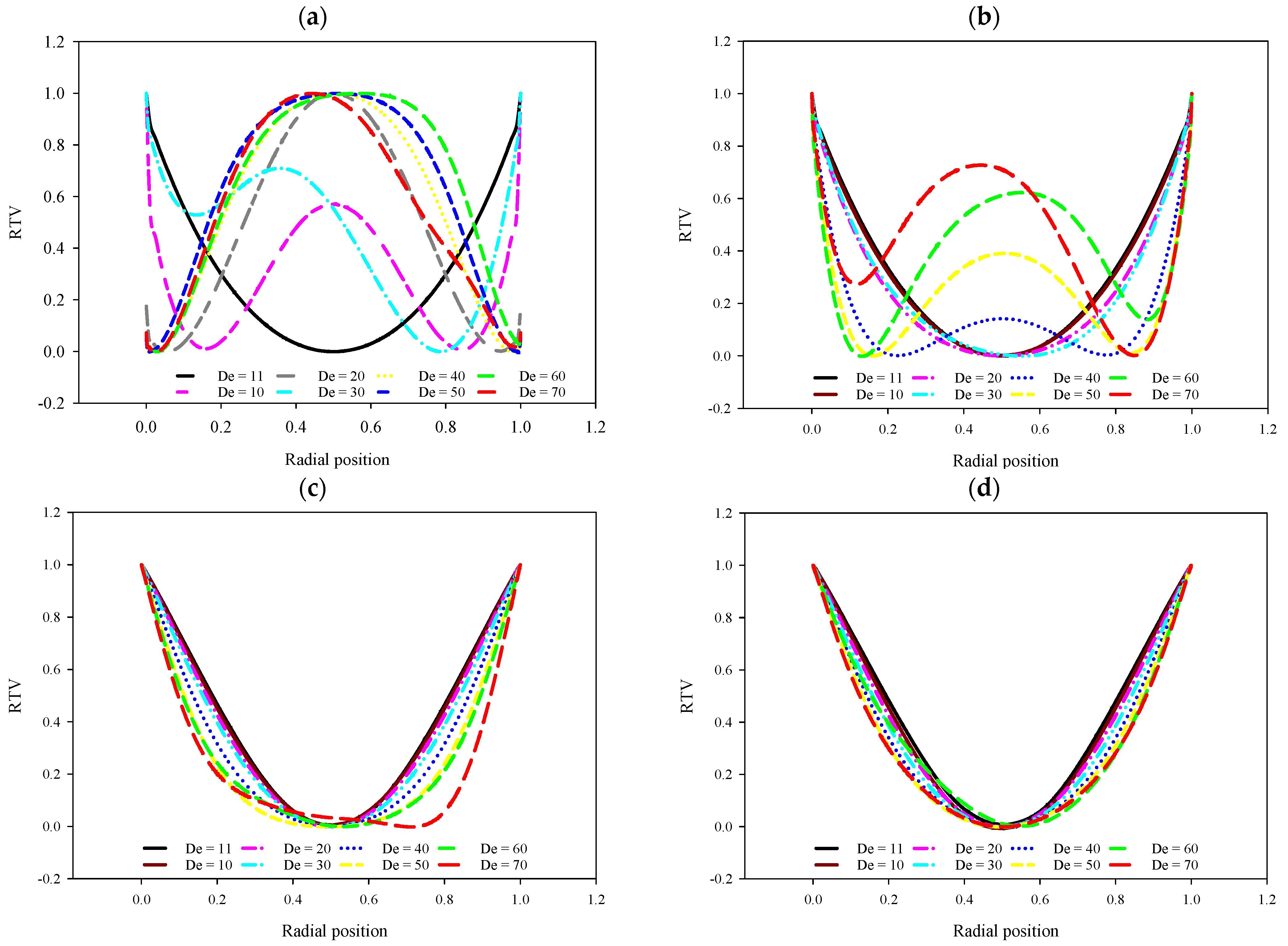
Figure 9 illustrates the RTV at different De over specific time intervals. The graphs are normalized, simplifying the comparison of trends across different Dean numbers. At 2 s, the fluid appears notably unstable, forming a parabolic shape only at D e = 11 , suggesting a specific stability threshold at this early stage. Moving to 4 s, D e = 10 , 20, and 30, exhibiting stability and forming parabola shapes which are indicative of potential full development, while the other Dean numbers do not follow this pattern. By 6 s, all the Dean numbers, except for 70, demonstrate stability, suggesting a transition to a more consistent flow pattern. Finally, at 8 s, all the Dean numbers stabilize and form parabolic shapes, indicating a fully developed and stable flow regime—characterized by consistent and predictable behavior over time, without sudden fluctuations.
In addition, it is noteworthy that at all time intervals, the De of 11 consistently exhibits a uniform and predictable profile, aligning closely with the input velocity shown in Figure 4. This stability ensures that the PIVG measurement can accurately capture the angular velocity at each time step. In contrast, higher Dean numbers exhibit fluctuations, resulting in less reliable measurements and potentially compromising the accuracy of the PIVG system. This highlights the significance of selecting an optimal Dean number, such as 11, to ensure consistent and reliable performance in capturing fluid dynamics within the toroidal pipe.
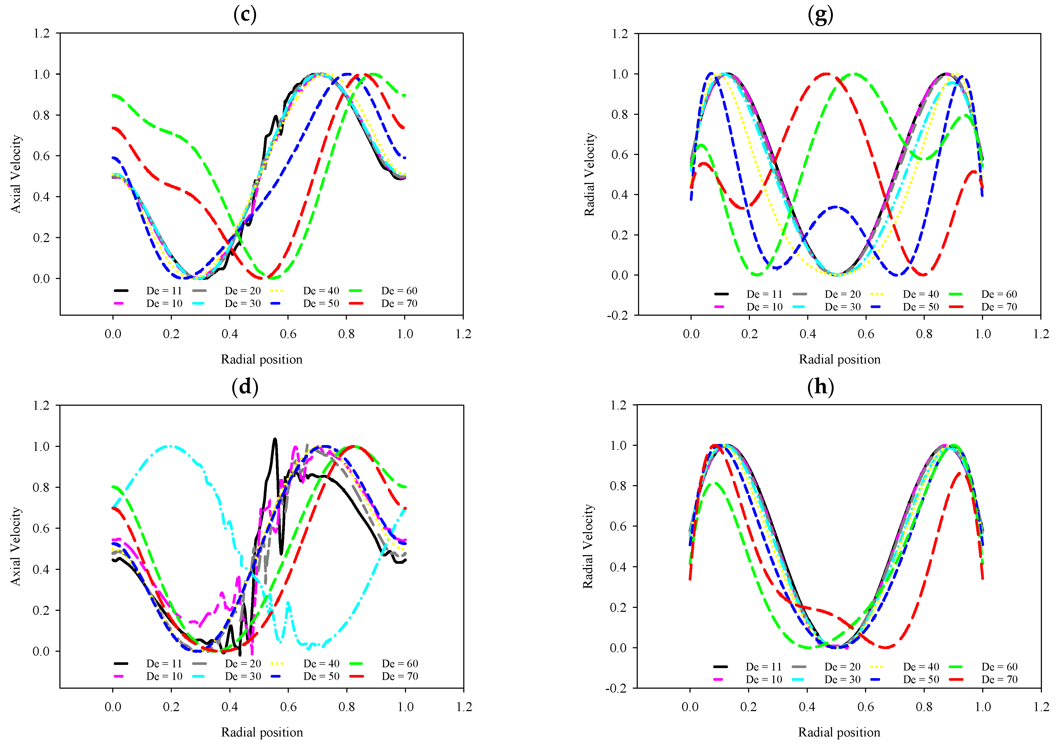
The normalized axial and radial velocity profiles are shown in Figure 10, which highlights the complex secondary flow patterns within the toroidal pipe at various Dean numbers. As mentioned, normalization enhances comparability, allowing a detailed analysis of these patterns. The axial velocity profile showcases consistent flow patterns at lower Dean numbers, resembling sinusoidal trends. This sinusoidal behavior signifies stable fluid movement along the toroid’s length. However, as the Dean numbers increase, especially around 70, the sinusoidal pattern becomes more frequent, indicating a higher number of oscillations within a given time frame. This increase in frequency implies intensified oscillatory behavior in the fluid’s axial and radial movements. Similarly, the radial velocity profiles, exhibit sinusoidal trends at lower Dean numbers, indicating predictable radial fluid movements. Yet, at higher Dean numbers, particularly around 70, the sinusoidal pattern becomes more rapid, signifying a higher frequency of radial oscillations. This observation emphasizes the complex fluid dynamics that accompany higher Dean numbers, leading to rapid and complex movements. Understanding these complications is crucial when researching secondary flows in many engineering contexts.

4.3.2. Optimal Fluid Dynamics at De = 11 for PIVG Operation

In this part, we consider the vital decision regarding selecting a De of 11 for the PIVG system. Our purpose is to illuminate the dependability and uniformity of fluid flow phenomena under these specific circumstances and to provide useful thoughts about the design and operation.
  • The RTV and Secondary Flow
In this section of results, attention is directed towards the optimization of the PIVG system, with a specific emphasis on the most pertinent Dean number, De = 11. This choice is pivotal for ensuring the ideal conditions for PIVG functionality and marks a crucial step towards enhancing the reliability and precision of the PIVG sensor. Additionally, it is important to note that the results presented in this section are not normalized, and they allow a clear distinction between the values of the primary and secondary flow.
In this 3D (Figure 11) graph the exponential increase in velocity until 4.5 s, followed by an exponential decrease until the end, confirms the correlation between the velocity distribution and the input angular acceleration rate. These findings further support the consistency between the numerical simulation and the expected behavior of the fluid flow inside the toroidal system. The stability is vital for the PIVG sensor’s accurate operation; regardless of the PIV’s position, it will yield consistent results. Furthermore, this finding underscores the suitability of the toroidal dimensions and fluid behavior for integration into the PIVG system.
The secondary flow at the De = 11 is shown here, and the velocity vector field on the radial cross-section of the toroidal pipe is displayed, offering insights into flow dynamics at different time steps, as shown in Figure 12. Velocity vectors intensify until 4 s, reflecting the toroidal system’s increasing angular velocity. A transformation occurs from 6 to 8 s; while the counter vortices are always present at all times, their intensity notably increases between 6 and 8 s. This evolution from outwards to inwards aligns with Dean’s curved pipe study [4,6,20], underlining the enduring relevance of his insights. Additionally, in Figure 13, the temporal evolution of the secondary flow (SF) at time intervals measured at radial positions r = 0 (center), r = 1, and r = 2 within the toroidal pipe is illustrated. Clearly, for all three radial positions, the secondary flow exhibits a consistent pattern of gradual augmentation from 2 to 4 s, culminating in a prominent peak at the 4 s mark. This peak is observed both at the center (r = 0) and progressively towards the outer radial positions (r = 1 and r = 2), accentuating the synchronized nature of this phenomenon across the toroidal pipe’s cross-section. Beyond this peak, the secondary flow gradually decreases at 6 and 8 s, indicating a consistent behavior across various radial positions.
The graph (Figure 14) presents a comparative visualization of two crucial flow aspects within a toroidal system: secondary flow and RTV. Remarkably, it is discernible that the secondary flow exhibits notably weaker intensity in contrast to the comparatively more dominant RTV. The noticeable difference in strength implies that the secondary flow can be disregarded, especially when using particle image velocimetry (PIV) to measure RTV, which is crucial for the function of the PIVG. The reduced impact of the secondary flow allows a simplified measurement process (i.e., u = v = 0). This simplification enables a direct and precise determination of fluid velocity specifically in the direction of relative tangential motion, rather than measuring in three dimensions using PIV techniques.
  • Pressure Distribution
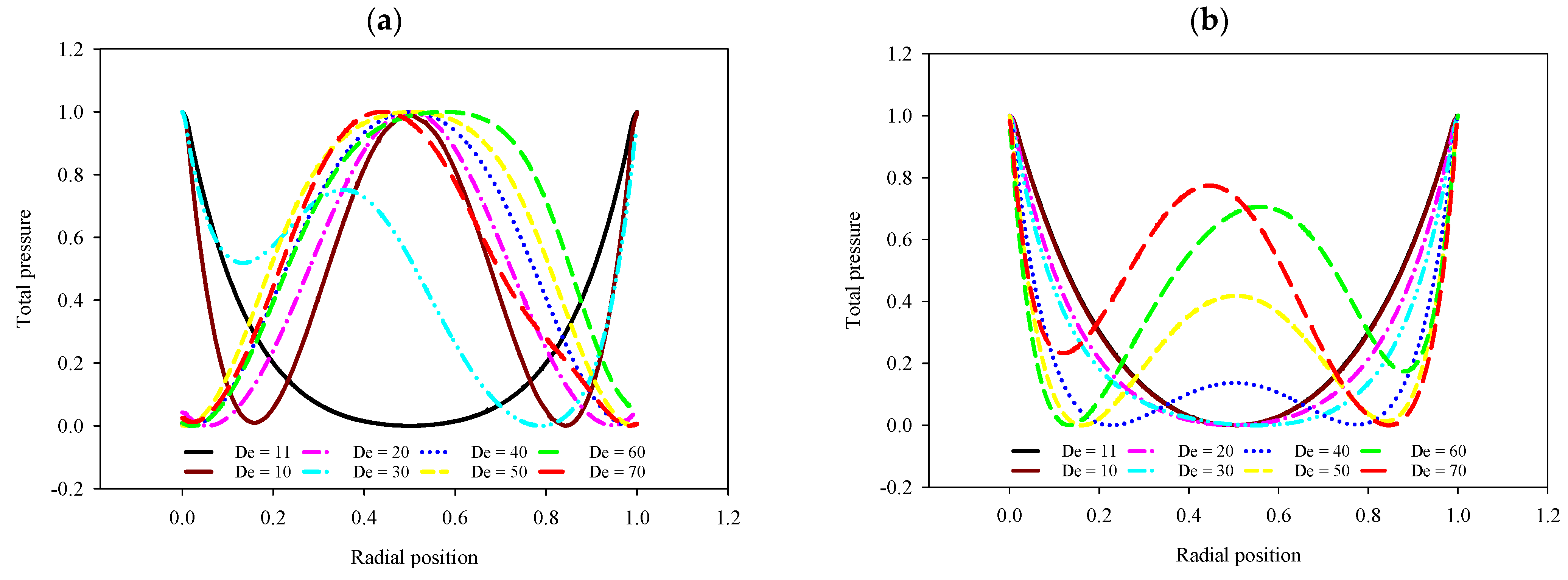
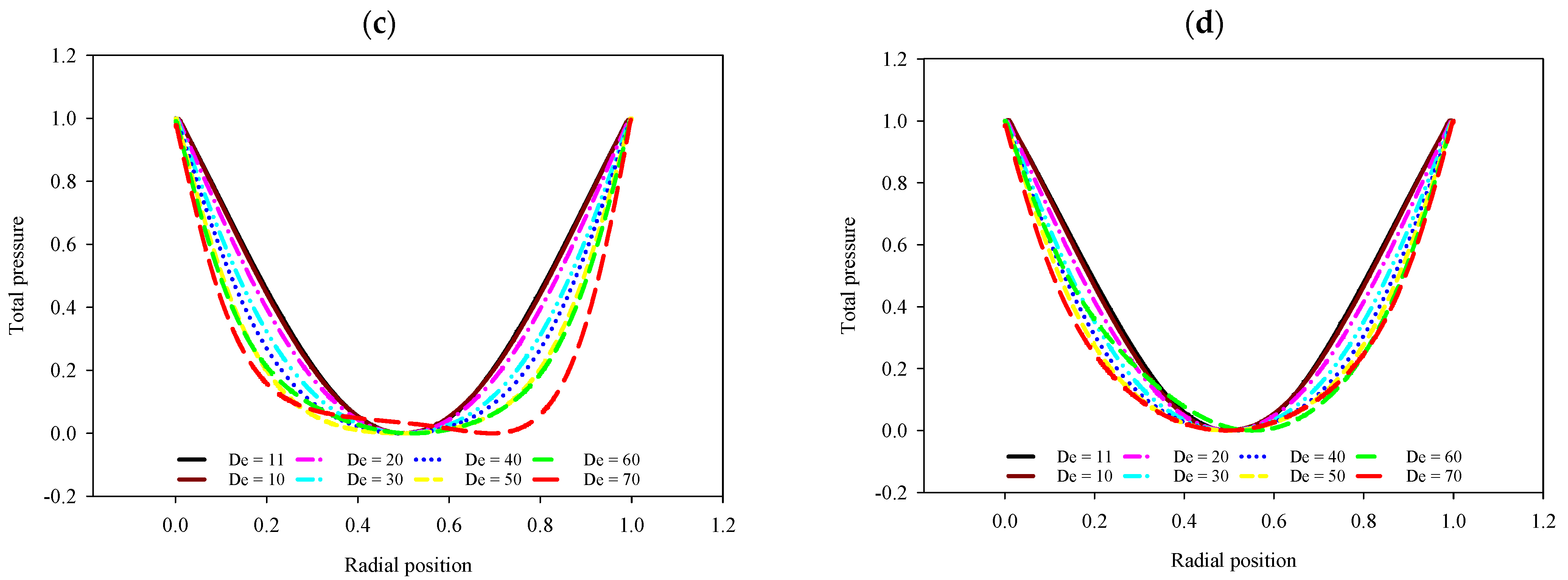
The examination of pressure along the curvature of the toroidal geometry in Figure 15 offers valuable insights into the fluid dynamics within the PIVG system. By measuring pressure at various angles along the curvature, we gain an understanding of how centrifugal forces are distributed within the toroidal vessel. The consistent pattern observed in the pressure gradient graph, with the gradient remaining close to zero across different angles, indicates a balanced distribution of centrifugal forces. This balance is attributed to the uniform curvature of the toroidal cross-section, which ensures consistent fluid behavior regardless of the angle of measurement. Importantly, the near-zero pressure gradient (∂P/∂ϕ = 0) signifies a stable fluid flow pattern, which is crucial for accurate and reliable performance of the PIVG. Understanding the pressure distribution along the toroidal curvature helps optimize the design of the PIVG system, ensuring uniform fluid behavior and minimizing disturbances that could affect angular velocity measurements.
From the CFD results, it can be inferred that the mathematical model, represented by the Navier–Stokes equation, for the PIVG sensor provides a wide domain of validity with high fidelity. However, ensuring that the fluid behavior aligns with the prescribed limits, particularly in terms of laminar flow with a low Dean number, is crucial for optimal PIVG performance. After analyzing a range of Dean numbers from 10 to 70, our study identified a De of 11 as optimal for achieving favorable fluid dynamics within the toroidal vessel. This finding has significant implications for the design of the toroidal geometry, as we pinpointed ideal dimensions characterized by a curvature radius of 25 mm and a cross-sectional diameter of 5 mm. These dimensions were found to promote stable and well-developed fluid flow patterns, which are particularly suitable for PIVG operation. With these dimensions identified, we can tailor the packaging of the gyroscope to ensure optimal performance and functionality, offering valuable guidance for decision making in the design and implementation of PIVG systems, thereby enhancing their effectiveness in inertial navigation applications.

5. Conclusions

In conclusion, our study, which is specifically tailored to the accelerated toroidal pipes utilized in PIVGs, stands as a cornerstone in the ongoing enhancement of navigation sensor technologies. The study examined several aspects, including a convergence study, validation, evaluation of the pressure gradients, and a detailed examination of relative tangential and secondary flows. The convergence study revealed notable differences, with the medium mesh exhibiting a higher uncertainty (GCI32%) than the fine mesh (GCI21%). The average uncertainty attributed to spatial discretization is 1.47% for GCI32% and 0.27% for GCI21%. In the validation phase, the study showed remarkable agreement with the experimental data, validating the accuracy of our simulations. This agreement establishes the domain fidelity crucial for PIVG performance. Our simulations have provided a viewpoint on an accelerated toroidal geometry, highlighting how the fluid behaves under this acceleration and different conditions, with Dean numbers ranging from 10 to 70, and we utilized a ramp profile as the input angular velocity for the toroidal pipe. However, the most stable configuration, which was particularly beneficial for PIVG applications, was identified at De = 11 due to its stable dynamic fluid behavior, aligning with the toroid’s specific dimensions. By selecting De = 11, we not only identify suitable dimensions for toroidal construction but also mitigate secondary flow effects, thus enhancing the precision and reliability of PIVGs in inertial navigation applications. Moreover, by selecting De = 11 and minimizing secondary flow, our study suggests the potential for a reduction in the mathematical model complexity and a focus on PIVG measurements based solely on primary flow dynamics; this offers a promising avenue for future research and practical implementation.

Author Contributions

Conceptualization, R.E.; Methodology, R.E.; Validation, R.E.; Writing—original draft, R.E.; Writing—review & editing, A.M.; Supervision, N.E.-S. and A.M. All authors have read and agreed to the published version of the manuscript.

Funding

This research received no external funding.

Data Availability Statement

The original contributions presented in the study are included in the article, further inquiries can be directed to the corresponding author.

Acknowledgments

The authors acknowledge the National Science Engineering Research Council of Canada (NSERC) for their support.

Conflicts of Interest

The authors declare no conflicts of interest.

Appendix A. The Results at Different De

Figure A1. RTV contour at (a) 2 s, (b) 4 s, (c) 6 s, and (d) 8 s and different values of De.
Fluids 09 00103 g0a1aFluids 09 00103 g0a1b
Figure A2. Radial velocity contour at (a) 2 s, (b) 4 s, (c) 6 s, and (d) 8 s and different values of De.
Fluids 09 00103 g0a2aFluids 09 00103 g0a2b
Figure A3. Axial velocity contour at (a) 2 s, (b) 4 s, (c) 6 s, and (d) 8 s and different values of De.
Fluids 09 00103 g0a3aFluids 09 00103 g0a3b

Appendix B. The Pressure Distribution at Different De

Figure A4 presents the pressure distribution profiles at various time points and different De, offering a comprehensive insight into the pressure behaviors within the toroidal vessel. Incredibly, the pressure trends mirror the patterns observed in the RTV profiles, indicating a significant correlation between fluid pressure and rotational dynamics. Notably, all the profiles have been normalized, ensuring a consistent basis for comparison. These findings have pivotal implications for applications such as the PIVG sensor, where understanding pressure dynamics is integral.
Figure A4. Pressure distribution at (a) 2 s, (b) 4 s, (c) 6 s, and (d) 8 s and at different De.
Fluids 09 00103 g0a4aFluids 09 00103 g0a4b

Appendix C. The Detailed RTV at Different Curvature Angle and Different Radius

The stability of the fluid dynamics at De = 11 is confirmed by a different approach. Figure A5a, representing the relative tangential velocity at the time interval of 2 s at varying curvature angles, offers an insight into the fluid dynamics within our toroidal system. A consistent trend emerges across the diverse angles examined, revealing a uniformity in the RTV within the toroidal pipe. As well as Figure A5b shows the RTV against time series at different cross-section radii.
Figure A5. (a) RTV at the different circumferential positions at 2 s, (b) RTV vs. time series at different cross-section radii.
Fluids 09 00103 g0a5

References

  1. Youssef, A.A.; El-Sheimy, N. Particle imaging velocimetry gyroscope. Sensors 2019, 19, 4734. [Google Scholar] [CrossRef] [PubMed]
  2. Elaswad, R.; El-Sheimy, N.; Mohamad, A.A. Review—Basic and Advanced Inertial Navigation Fluid-Based Technology. ECS Sens. Plus. 2023, 2, 023201. [Google Scholar] [CrossRef]
  3. El-Sheimy, N.; Youssef, A. Inertial sensors technologies for navigation applications: State of the art and future trends. Satell. Navig. 2020, 1, 2. [Google Scholar] [CrossRef]
  4. Norouzi, M.; Sedaghat, M.; Shahmardan, M. An analytical solution for viscoelastic dean flow in curved pipes with elliptical cross section. J. Non-Newtonian Fluid Mech. 2014, 204, 62–71. [Google Scholar] [CrossRef]
  5. Dean, W.R.; Hurst, J.M. Note on the Motion of Fluid in a Curved Pipe. Mathematika 1959, 6, 77–85. [Google Scholar] [CrossRef]
  6. Dean, W.R., LXXII. The stream-line motion of fluid in a curved pipe (Second paper). Lond. Edinb. Dublin Philos. Mag. J. Sci. 1928, 5, 673–695. [Google Scholar] [CrossRef]
  7. Ligrani, P.M. A Study of Dean Vortex Development and Structure in a Curved Rectangular Channel with an Aspect Ratio of 40 at Dean numbers up to 430; AD-A286 159 NASA Army Research Laboratory Contractor Report 4607; Army Research Laboratory: Adelphi, MD, USA, 1994. [Google Scholar]
  8. Greenspan, H.P.; Howard, L.N. On a time-dependent motion of a rotating fluid. J. Fluid Mech. 1963, 17, 385–404. [Google Scholar] [CrossRef]
  9. Weissenberg, K. The Theory of Rotating Fluids. Phys. Bull. 1968, 19, 426–427. [Google Scholar] [CrossRef]
  10. Van Dommelen, L.L.; Cowley, S.J. On the Lagrangian description of unsteady boundary-layer separation. Part 1. General theory. J. Fluid Mech. 1990, 210, 593–626. [Google Scholar] [CrossRef]
  11. Lam, S.T. On High-Reynolds-Number Laminar Flow through a Curved Pipe, and Past a Rotating Cylinder. 1988. Available online: https://hdl.handle.net/10044/1/47142 (accessed on 17 March 2024).
  12. Madden, F.N.; Mullin, T. The Spin-Up from Rest of a Fluid-Filled Torus. J. Fluid Mech. 1994, 265, 217–244. [Google Scholar] [CrossRef]
  13. Elaswad, R.; El-Sheimy, N.; Mohamad, A. Trajectory dynamics of particles in accelerated toroidal pipe: A computational study using CFD-DPM simulations. J. Comput. Sci. 2024, 78, 102285. [Google Scholar] [CrossRef]
  14. Zhou, Y.; Shah, S. Fluid Flow in Coiled Tubing: A Literature Review and Experimental Investigation. J. Can. Pet. Technol. 2004, 43, 52–61. [Google Scholar] [CrossRef]
  15. van Tiem, J.; Groenesteijn, J.; Sanders, R.; Krijnen, G. 3D printed bio-inspired angular acceleration sensor. In Proceedings of the 2015 IEEE Sensors, Busan, Republic of Korea, 1–4 November 2015; pp. 1–4. [Google Scholar]
  16. Groenesteijn, J.; Droogendijk, H.; de Boer, M.J.; Sanders, R.G.P.; Wiegerink, R.J.; Krijnen, G.J.M. An angular acceleration sensor inspired by the vestibular system with a fully circular fluid-channel and thermal read-out. In Proceedings of the 2014 IEEE 27th International Conference on Micro Electro Mechanical Systems (MEMS), San Francisco, CA, USA, 26–30 January 2014; pp. 696–699. [Google Scholar]
  17. Celik, I.B.; Ghia, U.; Roache, P.J.; Freitas, C.J.; Coleman, H.; Raad, P.E. Procedure for Estimation and Reporting of Uncertainty Due to Discretization in CFD Applications. J. Fluids Eng. 2008, 130, 078001. [Google Scholar] [CrossRef]
  18. Roache, P.J. Fundamentals of Verification and Validation; Hermosa Publishers: Socorro, NM, USA, 2009. [Google Scholar]
  19. del Pino, C.; Hewitt, R.E.; Clarke, R.J.; Mullin, T.; Denier, J.P. Unsteady fronts in the spin-down of a fluid-filled torus. Phys. Fluids 2008, 20, 124104. [Google Scholar] [CrossRef]
  20. Dean, W., XVI. Note on the motion of fluid in a curved pipe. Lond. Edinb. Dublin Philos. Mag. J. Sci. 1927, 4, 208–223. [Google Scholar] [CrossRef]
Figure 1. Toroidal coordinate system.
Fluids 09 00103 g001
Figure 2. Meshed computational domain.
Fluids 09 00103 g002
Figure 3. The input angular velocity for the toroidal.
Fluids 09 00103 g003
Figure 4. The relative tangential velocities function of different numbers of elements, at 2 s.
Fluids 09 00103 g004
Figure 5. Primary velocity vs. time series.
Fluids 09 00103 g005
Figure 6. (a) RTV contour, (b) radial contour, (c) axial contour at 2 s.
Fluids 09 00103 g006
Figure 7. (a) RTV contour, (b) radial contour, (c) axial contour at 4 s.
Fluids 09 00103 g007
Figure 8. (a) RTV contour, (b) radial contour, (c) axial contour at 8 s.
Fluids 09 00103 g008
Figure 9. RTV at different De (a) 2 s, (b) 4 s, (c) 6 s, (d) 8 s.
Fluids 09 00103 g009
Figure 10. Axial velocity (a) 2 s, (b) 4 s, (c) 6 s, (d) 8 s and radial velocity (e) 2 s, (f) 4 s, (g) 6 s, (h) 8 s, at different De.
Fluids 09 00103 g010aFluids 09 00103 g010b
Figure 11. The relative tangential flow velocity profile changes over time.
Fluids 09 00103 g011
Figure 12. The relative velocity vector colored by radial velocity, outer (left side), inner (right side) (a) 2, (b) 4, (c) 6, and (d) 8 s.
Fluids 09 00103 g012
Figure 13. RTV time series at different cross-section radii.
Fluids 09 00103 g013
Figure 14. SF and RTV at r = 0 (center).
Fluids 09 00103 g014
Figure 15. Pressure gradient at 2 s.
Fluids 09 00103 g015
Table 1. Mesh refinement strategy.
CoarseMediumFine
Element Size1.9309 × 10−41.4586 × 10−41.0319 × 10−4
No. of Element (m)427,680992,1602,803,600
Mesh SliceFluids 09 00103 i001Fluids 09 00103 i002Fluids 09 00103 i003
Table 2. Grid convergence index.
Radius (r)V3, CoarseV2, MediumV1, FineGCI21%GCI32%
2.4550.2461830.2508960.25190.7319154.488632
2.0050.937310.9439390.94530.2643891.678087
1.5091.49371.498811.50090.2557110.814675
1.01351.860931.867211.86810.0874870.803668
0.5182.071322.076582.07760.0901560.605268
0.02252.143352.147282.14960.1981920.437335
Disclaimer/Publisher’s Note: The statements, opinions and data contained in all publications are solely those of the individual author(s) and contributor(s) and not of MDPI and/or the editor(s). MDPI and/or the editor(s) disclaim responsibility for any injury to people or property resulting from any ideas, methods, instructions or products referred to in the content.

