
A Comparative Analysis of Sediment Concentration Using Artificial Intelligence and Empirical Equations

1
Department of Civil Engineering, University of Engineering and Technology, Taxila 47050, Pakistan
2
Department of Civil Engineering, College of Engineering, Qasim University, Buraydah 51452, Saudi Arabia
*
Author to whom correspondence should be addressed.
Hydrology 2024, 11(5), 63; https://0-doi-org.brum.beds.ac.uk/10.3390/hydrology11050063
Submission received: 2 March 2024
/
Revised: 20 April 2024
/
Accepted: 25 April 2024
/
Published: 27 April 2024
Abstract
:Morphological changes in canals are greatly influenced by sediment load dynamics, whose estimation is a challenging task because of the non-linear behavior of the sediment concentration variables. This study aims to compare different techniques including Artificial Intelligence Models (AIM) and empirical equations for estimating sediment load in Upper Chenab Canal based on 10 years of sediment data from 2012 to 2022. The methodology involves utilization of a newly developed empirical equation, the Ackers and White formula and AIM including 20 neural networks with 10 training functions for both Double and Triple Layers, two Artificial Neuro-Fuzzy Inference System (ANFIS), Particle Swarm Optimization, and Ensemble Learning Random Forest models. Sensitivity analysis of sediment concentration variables has also been performed using various scenarios of input combinations in AIM. A state-of-the-art optimization technique has been used to identify the parameters of the empirical equation, and its performance is tested against AIM and the Ackers and White equation. To compare the performance of various models, four types of errors—correlation coefficient (R), T-Test, Analysis of Variance (ANOVA), and Taylor’s Diagram—have been used. The results of the study show successful application of Artificial Intelligence (AI) and empirical equations to capture the non-linear behavior of sediment concentration variables and indicate that, among all models, the ANFIS outperformed in simulating the total sediment load with a high R-value of 0.958. The performance of various models in simulating sediment concentration was assessed, with notable accuracy achieved by models AIM11 and AIM21. Moreover, the newly developed equation performed better (R = 0.92) compared to the Ackers and White formula (R = 0.88). In conclusion, the study provides valuable insights into sediment concentration dynamics in canals, highlighting the effectiveness of AI models and optimization techniques. It is suggested to incorporate other AI techniques and use multiple canals data in modeling for the future.
1. Introduction
Canal irrigation plays a vital role in the economic uplift of many regions globally. Maintaining sustainable morphology of canals is a thought-provoking issue for design engineers and irrigation departments [1]. Sedimentation of canals is an acute problem for sustainable morphology where feeding rivers carry a lot of sediments, which are transferred to the canals taken off from upper river reaches. Hence, in-depth understanding of sediment concentration is of paramount importance in sustaining acceptable design parameters of irrigation canals. The behavior of various variables involved in estimation of sediment load is nonlinear and highly complex. Sediment consists of gravel, sand, silt, clay, or any other particulate matter transported by water. There is a possibility of sediment deposition on the bed of the canal, or water can erode the bed material. This phenomenon is related to three-dimensional flow and is difficult to formulate accurately. Researchers usually study the sediment load in rivers using two main approaches, as outlined in previous research [2,3,4]. The first method involves analyzing bed loads and suspended loads separately, treating them as distinct components of the total sediment load. Conversely, the second method combines both bed and suspended loads to calculate overall sediment concentration [5,6,7,8]. The choice between these approaches depends on various factors such as available data, required accuracy for design studies, and the characteristics of the riverbed being studied. For example, gravel-bed rivers primarily transport sediment as bed loads, whereas sandy-bed rivers see contributions from both suspended and bed loads [9]. Consequently, determining the most appropriate and robust approach for quantifying sediment concentration is complex, especially considering how additional hydro-morphological factors can introduce uncertainty into numerical model outcomes. In-depth understanding of incipient motion and shield’s function is of utmost importance.
There is a long history of understanding the sediment concentration phenomenon and estimating the total sediment load, which depends on bed load and suspended sediment loads. Several formulae have been developed to estimate the total sediment load in channels [5,10,11,12]. According to researchers, the predictability of most of these equations is questionable as these equations may perform comparatively better at one place but very poorly in another.
As described above, another important phenomenon related to sediment concentration is the incipient motion, which has been given high importance in the understanding of sediment concentration, bed level changes of channels, and sustainable design of channels. The movement of sediment particles is of random and stochastic nature, so it is always difficult to accurately predict at which flow conditions the sediment particles will start to move or deposit on the bed of the channel. Some researchers have used a shear stress approach with Shield’s diagram to describe the sediment concentration phenomenon [13,14]. Others have directly used the velocity approach introducing critical velocity, the non-silting non-scouring velocity. The probabilistic approach, stochastic studies, energy slope technique, stream power concept, and regression analysis have gained importance from time to time to deal with the sediment load. However, there is hardly any sediment load formula that can comprehensively and accurately be used for various situations. Thus, there is a need for continual evaluation and upgrading of sediment load formulae. As the transportation of sediment particles is highly complex, a single Froude number or Reynolds number or both cannot demonstrate the total sediment load under all situations of a channel. Hence, a regression equation derived from measured data to estimate the total sediment load became popular [15,16]. According to Cheng et al. [16], sediment load is changing globally. Most of the frequently used formulae of sediment load have been developed for different sediment-carrying capacities and hence need upgrading for the varied discharge and sediment conditions. They have derived an improved total sediment load formula for the Lower Yellow River and urged further research in this field of specialization. Sulaiman et al. [17] have investigated reliability of various equations for sediment concentration in Euphrates River Iraq. They have tested the performance of Ackers–White, Colby, Bagnold, Engelund–Hansen, Yang, and Shen and Hung [5,10,11,12]. According to the authors, different projects running near the banks have changed the regime of this river. Although these formulae are well-known and commonly applied, the Engelund–Hansen performed comparatively better than all other formulae. Shen and Hung exhibited an accuracy of only 11%, while Yang, Bagnold, Ackers–White, and Colby showed accuracies of 16%, 21%, 32%, and 32%, respectively. Only the Engelund–Hansen showed an accuracy of 84%. Another paper has evaluated sediment load formulae and confirmed the comparatively better performance of the Engelund–Hansen formula for simulating the morphological changes for channels in South Korea [18]. Avgeris et al. [19] has compared the performance of estimating total sediment load by various nonlinear regression equations and the Yang formula for Kosynthos and Kimmeria Rivers. According to the authors, the total sediment load estimated from various sediment concentration formulae generally varies significantly from one another and from the recorded data. Therefore, hardly any developed sediment load formulae have obtained widespread acceptance for accurately estimating the total sediment load. They found that even the well-established formula of Yang needs improvements, which they modified by regression on the basis of long data.
Formulas developed by calibrating parameters from established formulas using powerful optimization techniques can effectively predict sediment concentration under conditions similar to those from which the original formulas were derived. The application of regression techniques can be found widely to adjust available well-known sediment load formulae with specific topography different from those that were developed. Environmental and climatic changes have further created new challenges in water resources management [20]. These changes have versed the situation, necessitating adjustment to the parameters of existing equations to reflect current conditions accurately. The Upper Chenab Canal (UCC) takes off from Chenab River, which is a transboundary river. Various projects on this river can cause changes in the river regime, resulting in its aggradation or degradation. Consequently, the sediment supply and sediment concentration are altered, disturbing sediment balance of the canals taken from its downstream [21]. Any change made by India on the upstream of Chenab River directly impacts the sediment load in the UCC, which is taken from a place soon after the river enters Pakistan. This paper has investigated the sediment concentration in this canal on the basis of sediment data from 2012 to 2022 collected from Marala Head Works, Sialkot, Pakistan. A reduced gradient optimization technique has been applied to develop a new sediment load equation for this canal, which is the first objective of the present paper.
A summary of the above discussion shows that the deterministic sediment concentration models face great difficulty including the initial and boundary conditions, stochasticity, and non-stationarity of the stream flow. Hence, the prediction of sediment load in streams should also be investigated using artificial intelligence (AI) models that according to many researchers are proficient in tackling nonlinear relationships between water flow, sediment particles, and environmental variables [22,23,24,25,26]. For investigation of the detailed role of various features of sediment concentration using AI models, limited research is reported [22,27]. Therefore, the present study aimed to compare different AI techniques with the empirical equations for estimation of total sediment concentration in UCC. Hence, the second objective of the present research is to study the sediment concentration in UCC using AI models. Application of AI is really a daunting task in the field of sediment concentration in channels. An Artificial Neural Network (ANN) model has been applied to investigate sediment concentration for a dataset obtained from laboratory experiments [28]. Various AI models including Multi-Layer Perceptron (MLP) ANN, Random Forest (RF), Support Vector Regression, and Long Short-term Memory have been investigated for prediction of sediment load in Johor River, Malaysia [25]. A thorough review of AI model applications for the prediction of sediment load has revealed that further investigations are necessary for successful applications of AI models in this field of specialization. As stated above, the development of an accurate and generalized sediment concentration model is a demanding task for AI experts because of the multifaceted character of the sediment concentration phenomenon [29,30]. A comprehensive study is made in this paper applying 24 AI models to estimate the total sediment load in the UCC.
2. Materials and Methods
2.1. Geographic Location and Description of Canal Characteristics
UCC is one of the most important main canals of the Indus Basin Irrigation System of Pakistan, which helps to provide a major portion of water necessary for agriculture, food, and energy for the nation [31,32,33]. It is a perennial flow canal. Rice, wheat, maize, barley, and vegetables are the major crops of the two growing seasons including Rabi and Kharif. UCC has extraordinary characteristics because it is an irrigation as well as a link canal. It serves a large proportion of the population of Punjab province, Pakistan. Therefore, it is always a subject of continual research.
UCC originates from Marala Head Works constructed on River Chenab six miles downstream of its entrance from Jammu Kashmir state to Punjab (Pakistan) during 1905–1912 with a design capacity of 331 m3/s. After the independence of Pakistan, when supplies of Upper Bari Doab Canal taking off from Madhu Pur Headworks on River Ravi and Dipal Pur Canal taking off from River Sutlej from Ferozepur (Canda Singh Wala) Headworks were cut off by the Indian Government, supplies of these canals were supplemented through development of Bambanwala Ravi Bedian Dipalpur Link Canal from 1950–1953. In this connection to compensate for this increased supply of this link canal, the capacity of UCC was increased from 331 to 467 m3/s through widening of the canal. Old Marala Headworks was not capable of diverting such huge discharges through the canal due to technical reasons; therefore, model studies were carried out, and it was remodeled during 1965–1968 accordingly. The channel width (B) is 107 m with a bed slope (S) of 0.00015. The minimum and maximum discharge (Q) in the canal observed during these 10 years of data is 84.125 m3/s and 424.84 m3/s. The water depth (D) and water velocity (V) varied from 0.69 to 3.44 m and 1.07 to 1.47 m/s, respectively. The range of sediment particle diameter (d50) found in the UCC canal was 0.1 to 0.24 mm with sediment concentration ranging from 0.11 to 0.5179 g/L.
The Triple Canal Project off-taking from the left bank of the River Chenab at Marala barrage, district Sialkot (Punjab) also included UCC. This canal at its tail trifurcates into three channels, which are Banbanwala Ravi Bedian Depalpur Canal, Main Line Lower, and Nokhar Branch. The main function of these canals is to supply irrigation water to specific command areas of districts Sialkot, Gujranwala, Sheikhupura, Lahore, Kasur, and, partially, Hafizabad and Okara in addition to providing the surplus supply through Baloki Head Works to lower Bari Doab canal.
It has a gross command area of 0.62 mega hectares, out of which more than 63% is cultivable. The UCC command area is arid to semi-arid wherein the supply of irrigation water is imperative to sustain agriculture, in view of insufficient and scanty rainfall. This irrigation system consists of a main canal, branch canals, distributaries, minors, and watercourses. The layout of UCC and its branches, including the command area under study, is shown in Figure 1. The original design philosophy was to have protective irrigation over a large area without considering crop water requirements. The present strategy of the UCC system is to grow more crops, the resulting gap between canal water supply and crop demands to be met through groundwater abstractions. The UCC system was also expected to be effective and equitable, but studies have shown that there is great inequity in actual withdrawals between head and tail watercourses [34], which always attract research work on UCC.
2.2. Data Sources and Measures
This paper has investigated the sediment concentration in UCC on the basis of sediment data from 2012 to 2022 collected from Marala Head Works, Sialkot, Pakistan. The details about the B, S, Q, D, V, d50, and sediment concentration have been mentioned in Section 2.1 as given above. The channel details including its B, cross-sectional details, and S have been taken from drawings and topographic maps provided by Marala Headworks authorities. Q is measured using a rating curve with a gauge reading taken from the barrage site. Gauge reading and water levels are measured regularly, on a daily basis. Current meter data are collected from time to time to verify the canal discharge. Sediment-laden water samples are collected from the canal. A sediment-laden water collector of known volume is filled from a location of canal head regulator where hydraulic jump occurs, so that the sediment is fully mixed in water samples. These samples are analyzed in the laboratory for obtaining the sediment concentration. The sediment amount is measured partially by hydrometer analysis and partially by weighing the settled sediment in a glass beaker. From these data, the sediment concentration is calculated in g/L. A gradation curve is prepared from which d50 of sediment is estimated. The V is estimated in the data analysis phase. The authors have obtained the data by visiting the measurement site, having discussions with experts, visiting head works offices, collecting documents and drawing from the authorities, a thorough literature survey, and surveying the canal itself. To ensure the accuracy of the data, regular visits were conducted, and data related to on-site Q, D, gauge height, and sediment concentration were collected frequently in collaboration with the Marala Headworks team.
2.3. Data Analysis Methods
The methodology framework for analyzing sediment concentration in canals is given in Figure 2. In this paper, various state of the art methods have been used to study the sediment concentration in UCC, including AI. In AI, an internal-structural procedure performs training, validation, and testing processes. The data are divided into three parts; usually 60% is used for training, 20% for validation, and 20% for testing. This ratio may differ as 70%, 15%, and 15% for training, validation, and testing, respectively. A ratio of 50%, 25%, and 25% for training validation and testing, respectively, may also work. There are two types for division of the data in the ratio of 70%, 15%, and 15%, for example, or the other for training, validation, and testing. In one type, the ratio 70%, 15% and 15% is selected randomly, while in the other type the first 70% of data are used for training, the first half of the remining data (15% of the whole data set) are chosen for validation and remaining last part is used for testing. In the current study, the data were randomly chosen for training, validation, and testing as commonly employed by previous researchers such as [35]. For training, 60% of the total data set was used, while the remaining 40% (20% + 20%) was designated for both validation and testing purposes. It was ensured that the model was trained on sufficiently large portions of data by using this approach.
A thorough investigation was made combining AI techniques and empirical models. A total of 24 AI models were tested, including 10 training functions for double layer (DL) and triple layer (TL) ANN models, making a total of 20 different ANN models. Furthermore, two types of Artificial Neuro-Fuzzy Inference System (ANFIS), Particle Swarm Optimization (PSO), and RF models were employed to study the sediment concentration in UCC. Additionally, two empirical equations including Ackers and White total load formula and a simple equation developed from UCC data, were examined. General Reduced Gradient (GRG) optimization was used to identify parameters of the Ackers and White total load formula and a simple equation based on data of UCC. The efficiency of the models was tested using a variety of performance indicators, including coefficient of correlation ® values, along with four types of error metrics. Analysis of Variance (ANOVA) and T-tests were performed to choose the best of 26 models. Furthermore, the Taylor Diagram was also plotted to represent the performance comparison visually. A detailed description of all these models and techniques is given in the subsequent section for comprehensive understanding.
2.3.1. Artificial Intelligence (AI) Models
The application of AI in sediment concentration is becoming important because of its ability to handle the nonlinear behavior of various variables [23,25,26]. There are several emerging categories of AI models including ANN, ANFIS, hybrid ANN, and machine learning techniques [26,36]. ANN models usually have three phases/layers consisting of an input layer, hidden layer, and output. The elementary units of an ANN technique are responsible for performing controls with the help of some inputs. The output estimates at the initial stage are compared with the measured values of variables under consideration called targets. Certain weights are then selected to improve the accuracy of the predictions. This involves training, validation, and testing phases in such a way that the out matches with the target. A feed-forward process of hidden layers turns-out the backpropagation (BP) to produce precise results. A multiple-hidden layers-system is called an MPL [29,30]. A variety of training functions are found in the literature. The present research has tested 10 types of training functions both in DL and TL as given in Table 1. Number neurons have been selected through an exercise of hit and trial as per procedures listed in some published papers [37,38].
Adaptive Neuro-Fuzzy Inference Systems (ANFIS)
ANFIS encompasses a fuzzy inference system along with ANN. Predictions of various parameters are made by applying a hybrid technique of combining gradient descent, backpropagation, and a least-squares system [28]. ANFIS has been used in some past studies in the field of sediment concentration [39,40]. It is a highly useful and efficient tool for predicting continuous real functions in each domain. If–then rules and membership functions are used in the fuzzy part of this technique to establish a connection between input and output variables; hence, the ANN is used for training in a manner as described above. Two membership functions used in this research are described in Table 2.
Particle Swarm Optimization (PSO) and Random Forest (RF) Models (AIM23 and 24)
PSO is a state-of-the-art optimization in AI applications. A set of solutions is generated randomly in the search space, after which the most optimal global minimum/maximum is sought using frequent particles updates [41]. The method is becoming popular in water resources engineering due to its high accuracy in solving complex hydraulic problems. PSO is an efficient algorithm, and it takes a comparatively low volume for computation, has a high probability of finding a global optimal solution instead of trapping into a local optimal solution, and has a very high rate of convergence [41,42,43].
RF is a powerful AI technique that can tackle both regression as well as classification problems [44,45,46]. Its algorithm is based on supervised learning, building a forest of decision trees in the training phase, which is highly useful in reaching the optimal solution [44]. In building every decision tree, a subset of features is randomly selected from the full feature set making the technique a robust one.
Input Combinations (IC) for Artificial Intelligence (AI) models and Sensitivity Analysis of Parameters
Various combinations of input variables for sediment load have been tested using the best AI model. The results of sediment load estimation are highly dependent on input data. The beauty of AI techniques lies in the fact that these models build a relationship between the input data and the output even when dealing with complex relationships that may not be easily expressible through formal equations. Therefore, selecting an appropriate combination of input parameters is an imperative step in AI model applications. A total of 9 input combinations (IC1–IC9) have been selected in AI models with varying combinations of Q, D, V, and d50. The following IC of variables (Table 3) were tested one by one, and the optimal combination has been highlighted in this paper.
2.4. Ackers and White Total Load Formula and Developed Equation
2.4.1. Ackers and White Total Load Formula
Ackers and White used extensive data from sediment concentration experiments to find the total sediment load formula. The formula requires five steps to the total sediment load:
- Computation of a dimensionless particle size parameter:
In the above equation, P(Dgr): dimensionless sediment diameter, d50: sediment particle diameter (sediment size in a distribution, for which 50% by weight is finer), g: gravitational acceleration, s: specific gravity of sediment, and : kinametic viscosity of water. For uniform grain sizes, the mean sediment diameter, d50, is used. For graded sediments, the d35 is used.
- 2.
- Compute four parameters, P(m), P(n), P(A), and P(C), to be used later:
If P(Dgr) > 60, the particle sizes are said to be coarse:
where P(n), P(A), P(m), and P(C) are the parameter/coefficients in the Ackers and White technique. If P(Dgr) is less than 60, but larger than 1, the sediments are medium sized:
P(n) = 0.0 P(A) = 0.17 P(m) = 1.5 P(C) = 0.025
If P(Dgr) is less than 1, the sediments are under 0.04 mm. It is assumed that cohesive forces may occur, making it difficult to predict the sediment concentration. However, the sediment concentration is then usually much larger than what is available for the river, so the sediment load is limited by the supply.
- 3.
- The mobility number is then computed (note simplification if n = 0):
In Equation (4) P(Fgr): mobility number, V: flow velocity, : shear velocity, g: gravitational acceleration, n: Acker and White coefficient, : density of sediment, : density of water, d50: sediment particle diameter, and D: water depth.
- 4.
- The sediment concentration, c, is then given in weight-ppm
- 5.
- The concentration is multiplied with the Q (in m3/s) and divided by (10)3 to get the sediment load in kg/s.
2.4.2. Developed Empirical Equation
As described above in various sections, the sediment concentration is a highly complex phenomenon and there is no universal formula that can be applied for various channels with high accuracy. Every time for every channel, one has to choose the best formular applicable to the given situation. After choosing the best equation, there is again a need to optimize the parameters of the sediment load equation by applying a strong optimization scheme. In this paper, it is thought to develop a simple total sediment load equation having fewer but catch-all type parameters that may handle the complex relationship between the sediment concentration variables. The developed equation is of the form as given below:
where Qs is sediment load, V is flow velocity, D is water depth, α, β, and γ are the parameters of the equation, which have been optimized using General Reduced Gradient (GRG).
2.5. General Reduced Gradeint (GRG), an Optimization Tachniques
Empirical equations of sediment load often require the identification of their parameters most of the time for accurately modeling sediment concentration phenomena. Therefore, optimization techniques have great importance in the field of sediment concentration. There are many optimization techniques available in the literature. GRG is recognized as a state of the art and efficient optimization technique [47]. GRG stands out for its user-friendliness, high efficiency, ability to search global minimums without wasting time being trapped in local optimal solutions, and takes the minimum possible computer memory for computations. Non-linear problems regarding the Acker and White equation have been solved by applying GRG to optimize two parameters of the formula. The same technique is used to calibrate a simple sediment load formula developed in this paper. The main goal of GRG is the global maximization of R or minimization of the objective function based on Mean Square Error (MSE) estimated from simulated and observed sediment concentration. Figure 3 illustrates the flowchart of the GRG process.
2.6. Performance Evaluation
Five performance indicators, coefficient of correlation (R), Mean Square Error (MSE), Mean Absolute Error (MAE), Sum of Square Error (SSE), and Sum of Absolute Error (SAE), were used to assess the degree of accuracy of predictions resulting from the methods mentioned above. The following equation gives the formula for R [48]).
presents recorded sediment discharge/sediment concentration for the ith measured value, denotes predicted discharge/sediment concentration for the same data point, is mean discharge/sediment concentration, and n is the total data points used for the models’ testing.
The MSE was estimated using the following equation:
The MAE is given by the following equation.
The SSE is given by the following equation.
The SAE is given by the following equation.
2.7. Analysis of Variance (ANOVA), T-Test and Taylor’s Diagram
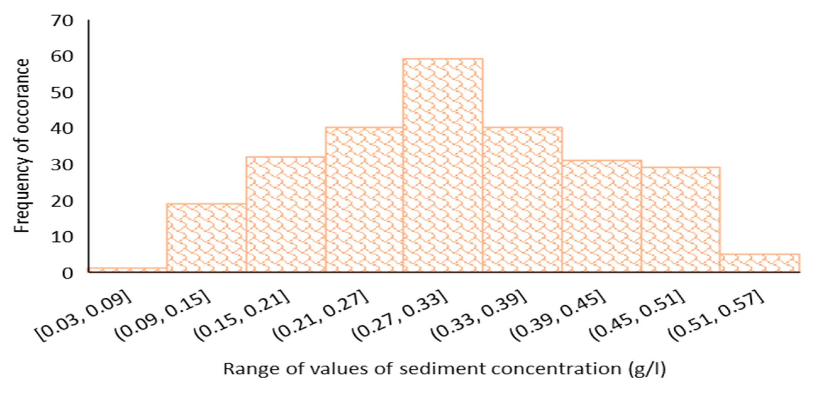
T-tests and ANOVA serve as the statistical bread-and-butter in basic science research [49]. ANOVA, a statistical technique employed to compare means among three or more groups, is considered an omnibus test statistic [50,51]. A significant p-value in ANOVA indicates that there is at least one pair where the mean difference is statistically significant. The ANOVA and T-test were performed using R-values to compare different models. A key requirement for both tests is that the observations should be independent and normally distributed. Both conditions are met in the present study as the histogram of sediment concentration values shows that the data are normally distributed (Figure 4). In the present study, as a first phase based on the overall performance, one model out ten DL ANN models showing the best performance, indicated by the highest overall R-value, is taken as the basis of the T-test and ANOVA. This model is compared with the other 9 models. Similarly, in the second phase, the best-performing model among the 10 TL ANN models was compared to the remaining 9 TL ANN models. Subsequently, the 2 best models out of the 20 ANN models were compared against the remaining models, including AIM21, AIM22, AIM23, AIM24, Emp-equ-1, and Emp-equ-2. Finally, the results obtained from ANOVA and T-test are then confirmed by Taylor’s Diagram.
Taylor’s Diagram was developed by Taylor (2001) and is a graphical tool to illustrate the similarity between two datasets. Taylor’s Diagram was developed to illustrate the relationship between the measured standard deviation (x-axis), simulated standard deviation (y-axis), and R (radial axis). The objective is to assess how closely the test field resembles the reference field. In a single (2D) Taylor diagram, a point on the graph signifies the root-mean-square error (RMSE), R, and the ratio of standard deviations between the actual and predicted data [52,53]. The performance of various prediction models has been tested by various authors by constructing Taylor’s Diagram [52,53]. Taylor’s Diagram shows the relationship between standard deviation, R, and RMSE.
3. Results
3.1. Evaluating Model Performance and Comparisons
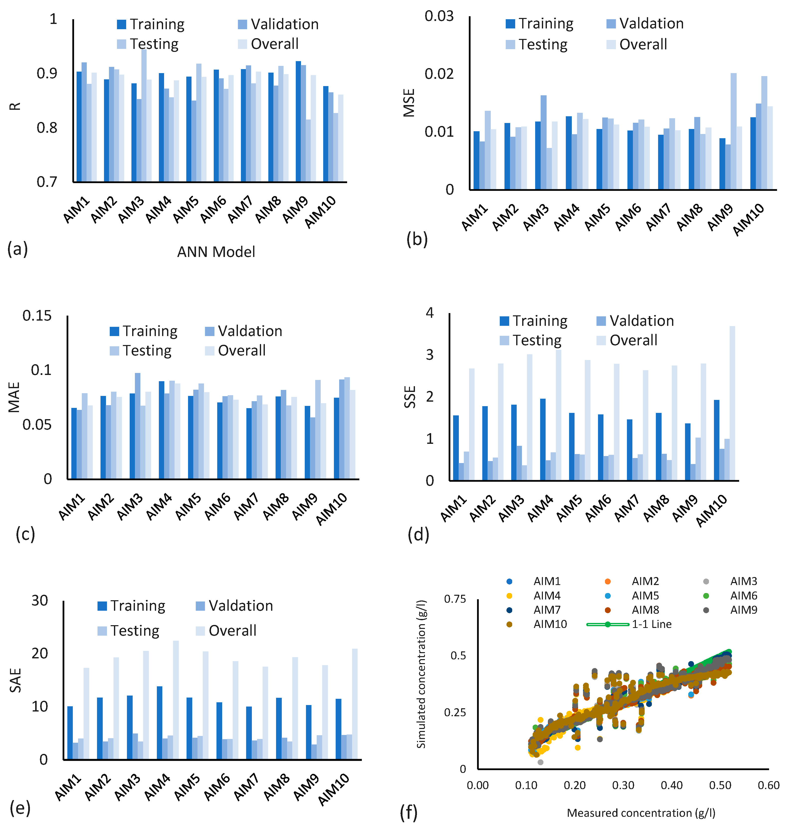
Ten different training functions as described in Table 1 have been tested with 10 neurons in each of the two hidden layers. Figure 5a–e shows the results from various angles. Figure 5a compares all ten training functions with respect to the R values. All the 10 models performed well because the values of “R” ranged from 0.81 to 0.94 in the testing process. Overall values of “R” are in the range of 0.86 to 0.90. Four types of results are shown in Figure 5a regarding R values in training, validation, testing, and overall. Based on these four values of R, it is difficult to decide which model has the best performance. Training, validation, and testing based on randomly chosen data sets usually provide such varying values of R. However, the models AIM1 and AIM7 have nearly similar performances and can be chosen as comparatively better performing models based on the overall values of R.
Figure 5b–e show the performance of models in terms of various types of errors. Figure 5b gives comparative values of MSE, Figure 5c,d provide MAE and SSE respectively. Considering errors as performance criteria, all the models have high performance. The results (Figure 5b) show a maximum value of MSE as 0.02. Other error values (Figure 5c–e) are also in the acceptable range (maximum values of MAE = 0.097, SSE = 3.69, and SAE = 22.45). Unexpectedly, the overall values of SAE are very high. Figure 5f presents graphs between measured and simulated sediment concentration from various models. All the models have results close to the 1:1 line, showing high performance in simulating sediment concentration from the UCC except model AIM10.
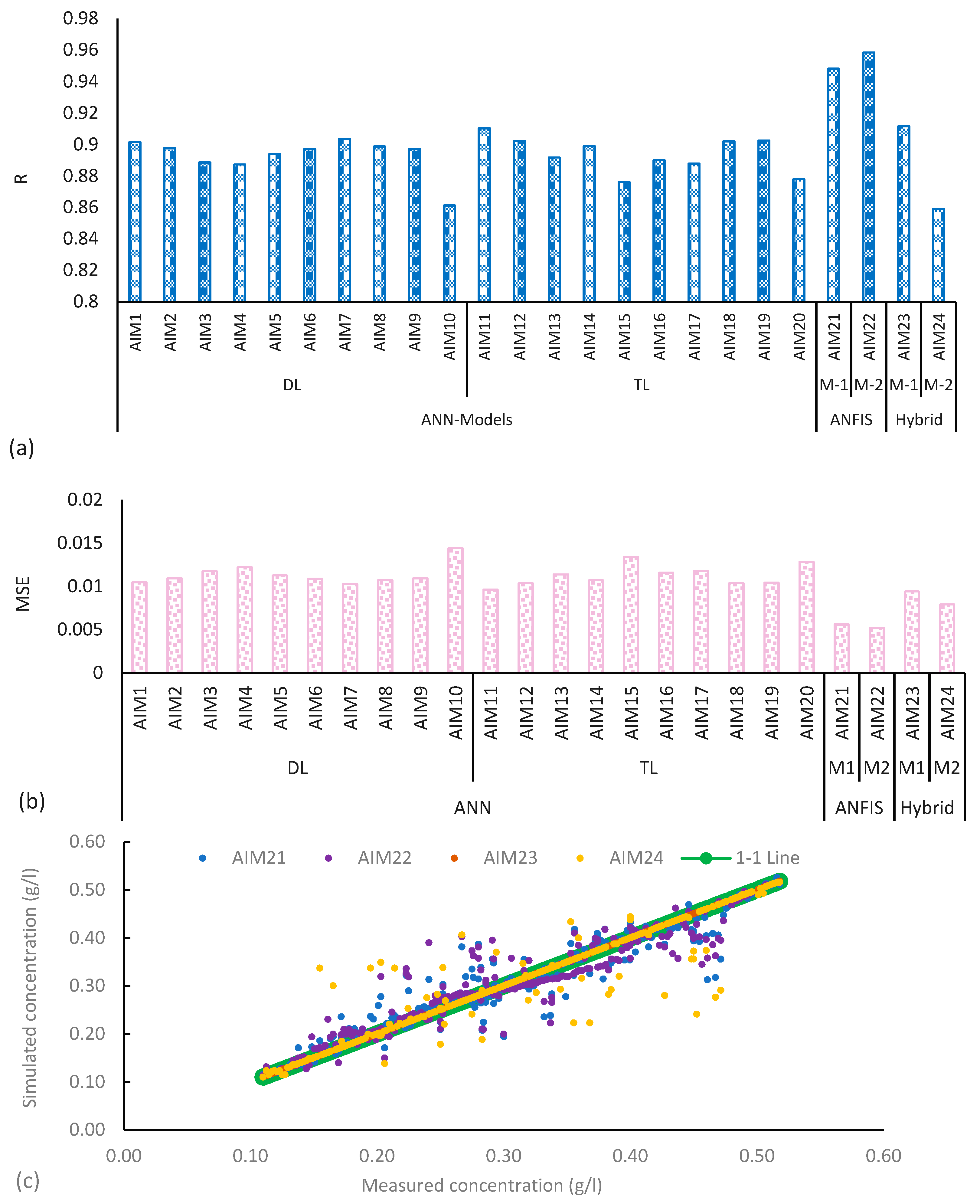
TL ANN models, utilizing the same training functions as the previous section, were examined next. Only two performance indicators, R and MSE are shown here in Figure 6a,b. However, it is a dual-purpose figure, and it shows the performance of TL ten training functions and compares DL with TL models. R values, ranging from 0.79 to 0.94, indicate strong model performance. TL ANN models have simulated sediment concentration that is comparatively better than that of DL ANN models. MSE values remain within acceptable ranges despite variations across training, validation, and testing phases. Notably, overall R and MSE values are estimated on the basis of the whole range of the data set of measured and simulated sediment concentration. According to Figure 6c, which gives a plot between measured and simulated sediment concentration from various models, the AIM11 model has results close to the 1:1 line. It means that AIM11 produces high accuracy in simulating sediment concentration from the UCC.
Figure 7a,b shows the impact of the number of neurons in hidden layers. The same number of neurons were selected for each of the two and three layers of DL and TL models. It is observed that the number of neurons in the hidden layers of DL and TL has a very small impact on the performance of models. The average value of the R is 0.895, the maximum is 0.926, and the minimum R = 0.819. The average value of MSE is 0.011, the minimum MSE is 0.0079, and the maximum is 0.018. It can be seen from Figure 7 that a large variation in R values occurs in the case of the AIM7 model and the highest value R of is obtained in the case of 38 neurons in each layer of the TL model AIM11.
Two ANFIS and two hybrid ANN models including PSO and RF are compared in this section with the help of overall values of R and MSE as given in Figure 8a,b. The values of R plotted in Figure 8a show very high performance of the two ANFIS and two hybrid ANN models. ANFIS AI models have simulated sediment concentration comparatively better than that of the hybrid ANN models. Figure 8b shows the MSE values for all four models, which show comparatively better accuracy than the ANN models described in previous sections. Figure 8c presents a plot between measured and simulated sediment concentration from various ANFIS and hybrid ANN models. The model AIM22 (ANFIS 2) and hybrid model AIM24 have results close to the 1:1 line, showing comparatively higher accuracy in simulating sediment concentration from the UCC.
The performance of two empirical sediment load equations is shown in Figure 9a,b. The R values are in the range of 0.88 and 0.92 for calibration and 0.7 to 0.65 for validation of equations. Figure 9b shows slight deviations of sediment concentration from the 1:1 line both in the case of the developed and Acker’s and White equations.
3.2. Input Combination (IC) Scenarios
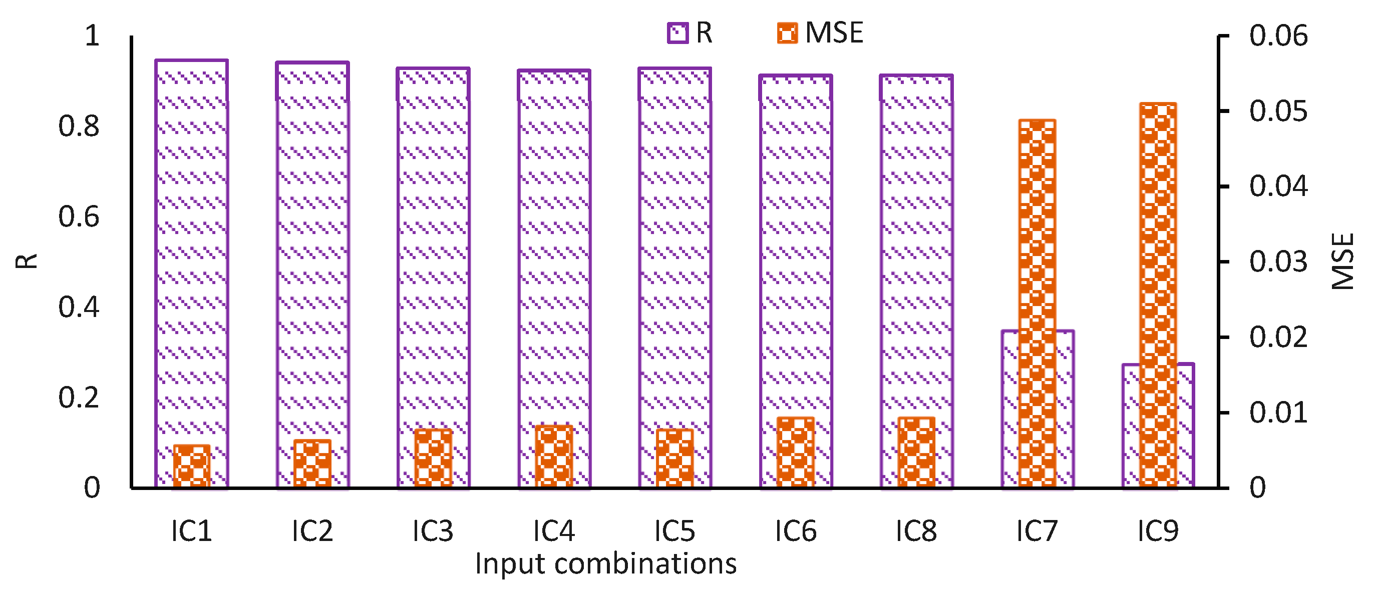
Figure 10 presents the performance of models with various IC. IC1 consists of all variables including Q, D, V, and d50 and produces the highest R value of 0.946 and minimum MSE = 0.0056. The second top merit combination is the IC2 having Q, D, and V as input variables. The results of sediment load simulations are in very good range from IC1 to IC7 (R values above 0.9 and MSE less than 0.0093). The worst results are obtained from IC8 and IC9. The reason for such results is explained in the discussion section.
3.3. Result of Analysis of Variance (ANOVA), T-Test, and Taylor’s Diagram
Figure 11a–d shows results of ANOVA, T-Test, and Taylor’s Diagram. In the present study, based on the overall performance, the AIM1 and AIM7 shows the best performance out of 10 DL ANN models, indicated by the highest overall R (Figure 11a,b). The ANOVA and T-Test were performed using R values for comparing different models. In the first phase of comparison, the AIM7 model was selected for comparison with other models, including AIM1 to AIM10. The choice of the AIM7 model was based on its overall R value, which was greater compared to those of the other models. Upon comparing AIM7 with different models, it is observed that AIM7 exhibited statistically significant differences with AIM1, AIM2, AIM4, and AIM9. The p-values obtained from the ANOVA test for these comparisons were below the range of p-values (0.05). Taylor’s Diagram in Figure 11b also confirms these results. In the second phase, the AIM11 model was compared to AIM12 through AIM20. The results of the comparison indicate that the AIM11 model has a significant difference with models AIM12 through AIM20. The p-values for these comparisons were below the confidence level (which was considered 5% for the p-value of T-test and ANOVA). When both these models, AIM7 and AIM11, were compared to the remaining models, including AIM21, AIM22, AIM23, AIM24, Emp-equ-1, and Emp-equ-2, the results showed significant p values for the models AIM21 and AIM22, which also have the higher values of R = 0.948 and 0.958, respectively. The overall results of ANOVA and T-test indicate that AIM11 performed better than other models. Figure 11c,d also show similar results keeping AIM11, AIM21, and AIM22 in top positions.
4. Discussions
Section 3.1 describes results from 10 DL and 10 TL ANN models. The performance of all the models is in the “very good” range because all values of “R” are greater than 0.75. These results are in line with past studies [28,53]. According to past research, the performance of models can be considered very good if R values lie in between 0.75 to 1 [47,48,49]. The R values also lie in the performance acceptance range given by [39,40,41]. The results of the models are in line with previous studies [54,55]. Correlations coefficient R values up to 0.98 for the application of AI models on sediment concentration have been obtained in past research [41]. However, the results of the present study are varied over a long range in training, validation, and testing phases. In some cases, the values of R become higher in training and low in testing and validation, while other cases have resulted in higher values of R in testing or validation as compared to that of training (Figure 5 and Figure 6). The values of R and various errors estimated for the whole data set (overall R, MSE, MAE, SSE, and SAE) are different than those of training, validation, and testing. The reason is that the data sets for training, validation, and testing have been chosen on a random basis. If the data set is uniform and ideal with no errors, then one can expect all values of performance indicators to be logical and have some relationship between overall R and errors values with those of values in the training, validation, and testing phases of these parameters. Due to this reason, the best model out of the 26 models tested in this research was selected based on performance indicator such as values of “R”, and a similar trend was adopted in previous research [47,48,49,53]. An easy way of selecting the best model is adopted in Section 3.1, where the selection of the best model is based on only the overall values of the performance indicators instead of considering all the phases of training, validation, and testing, as a similar trend was noticed in the prior studies [28,53]. However, it is not acceptable to some researchers, and hence additionally, ANOVA, T-Test, and Taylor’s Diagram have been used in this study [41,50,51,52].
The performance of the developed equation on the basis of GRG optimization and the Ackers and White total sediment load formula is the in acceptable range as per criteria given by some researchers [55,56,57]. The effectiveness of empirical equations falls short when compared to AI models. Understanding sediment concentration is a complex three-dimensional challenge. Deriving a universal formula for total sediment load proves difficult. Thus, GRG emerges as a valuable tool for recognizing the parameters of total sediment load formulas. In conclusion, optimizing parameters through GRG can notably enhance the performance of the Ackers and White formula for total sediment load. The empirical equation devised for total sediment load in UCC, utilizing the optimization scheme GRG, demonstrates superior efficiency over the Ackers and White total sediment load formula.
It is given in the results section that the IC1 consisting of all variables (Q, D, V, and d50) has comparatively higher performance of models in simulating sediment concentration in UCC. A value of R in the range of “very good” is obtained (R = 0.946 and MSE = 0.0056) (Figure 10). The second combination IC2 having Q, D, and V as input variables stands second in merit position with respect to the model performance. The overall performance of models for sediment load simulations is in the very good range from IC1 to IC7 (R values above 0.9 and MSE less than 0.0093), whereas the worst results are obtained from IC8 and IC9. It is understandable that excluding d50 from input variables does not make any significant difference in the efficiency of the models because it is the least impacting variable. It is very important to note this aspect of data of sediment concentration in UCC. Usually, d50 is a very important parameter in sediment concentration. Sediment particles with smaller mean diameters are easily removed from the bed of the channel even with comparatively smaller velocities of fluid and vice versa. Here in UCC, the case is slightly different. The sediment concentration and nature depend upon the situation in Chenab River. In the present study, it is observed that the sediment entering UCC has very small variations in d50 most of the time due to the constant S and smaller variation in V, and a similar mechanism was noticed in previous research [58,59]. Hence, this is the least influencing variable on simulation of sediment load variations. The same is the behavior of velocity in total sediment load estimations for various conditions in UCC. The S is nearly constant in canal reach under study. Hence there is a very small change in V even if the Q is changed. The changes in Q are encountered by changes in D. As a result, the sediment load variations are directly related to the Q and D in UCC, and previous research observed similar mechanisms under different flow conditions in the Upper Mississippi River [58,59]. Total sediment load in UCC changes mainly with changes in gauge height, Q, and D. Hence, the most influencing variable in the simulation of total sediment load is Q. The second most important variable is the D (Figure 10). The results of sediment load simulations are in the very good range from IC1 to IC7 (R values above 0.9 and MSE less than 0.0093), and this result aligned with previous research findings on suspended sediment load in the river [59]. The prediction results of total sediment load show poor performance of models from combinations IC8 and IC9. It is because of this reason that d50 and V are the least influencing variables regarding sediment load variations as explained above. These results are in contrast with those reported by Karami et al. [41]. The reason behind this issue is that they have used a different set of data where the V is the most influencing variable because they are using different S, which causes changes in V and corresponding sediment load, whereas in the present study, the S of UCC under study is constant and insignificant changes in V. However, their results regarding Q and D being significant variables in sediment load estimation match with the results of the present study.
The present study has mainly focused on addressing the challenges specific to the UCC, which is providing water to produce food and energy for a significant part of the population of the Punjab Province, Pakistan. Although it looks like a local scale analysis, its importance is high because of its relation to a global issue. There is a problem of sediment concentration in the UCC canal, and every year enormous expenditure is involved in the dredging of canal sediments in some reaches and maintenance of the foundation of hydraulic structures in the reaches where there is scouring. Therefore, an attempt has been made to thoroughly investigate the sediment concentration so that remedial measures can be proposed in the future. Similar studies have shown that local-scale analyses can contribute significantly to the understanding of larger-scale processes and inform broader scientific principles [60,61]. Our aim was to develop a sediment load equation fitted to the unique characteristics of the UCC canal. The results of the study will be important for the engineering community in general and especially in the Punjab Irrigation department in managing sediment concentration in canals.
It is worth noting that this manuscript has tested multiple models covering a wide range of aspects of AIM. For the sake of completeness of this case study, we have checked the influence on sediment concentration of some variables that have even insignificant impact. We aimed to provide a comprehensive evaluation of different methodologies comprising AIM and empirical equations to identify the most effective approach for sediment concentration prediction in the given context. The main purpose for testing many different combinations in AIM is that we wanted to check the impact of various parameters on the performance of AI models. While it may appear redundant that almost all models performed well, such thorough analysis ensures robustness and reliability in our findings. Similar studies have adopted this approach to ensure a rigorous assessment of model performance and to identify the most suitable techniques for specific applications [62,63]. One reach of the canal has been selected that has a uniform value of S. Therefore, in this case study, S being uniform has not been included in the IC of the AI models. Nevertheless, it is an important parameter in the Ackers and White and other total sediment load formulae. The d50 of sediment varies from 0.1 to 0.24 mm. Due to its insignificant variation in size in present study, it has negligible impact on sediment analysis, but it was necessary to confirm it by including it in the IC. However, it is important to note that even in seemingly uniform environments, variations in other parameters or boundary conditions can still significantly influence sediment concentration dynamics. Our discussion of these variables in the manuscript aims to provide transparency and insight into the limitations of our study, rather than dismissing their relevance outright.
The study included 26 models, 9 combinations of variables, and 5 performance indicators. However, as mentioned in the previous sections, we wanted to check the performance of AIM by trying different combinations. The inclusion of multiple AIM, combinations of variables, and performance indicators was aimed at providing a comprehensive evaluation of sediment concentration prediction techniques. Out of 26 models, the best model has been selected based on R value and MSE value. Additionally, statistical tests including T-tests and ANOVA tests have been utilized to evaluate the significance of differences between the best model and the remaining models as shown in Figure 11a. For all the DL ANN models, we compared the R value of AIM7 with the remaining DL models, and for TL ANN models, we compared the ANN 11 model with the remaining TL models. The hypothesis is that there is significant difference between the R value of AIM7 and AIM11 and all the other models (p value < 0.05). Figure 11a clearly shows that most of the models show a p-value less than 0.05 against ANOVA test and T-Test. Thus, we believe that statistical models perform differently. This approach of inclusion of many different combinations in models allow for an absolute exploration of the effectiveness and robustness of different methodologies, assuring that our conclusions are robust and reliable, as the same approach has been employed by past researchers [62,63].
It is worth mentioning that the study focused on the data related to a specific canal, the UCC, which has different dynamics as compared to rivers. Previous studies such as those by Almubaidin et al. [64], Kang et al. [65], and Nda et al. [66] have also investigated sediment concentration for similar cases. Their findings support the relevance of utilizing specific hydraulic conditions, like those of the UCC, to assess model performance critically. All the empirical equations have been developed to cover a wide range of data and incorporate the complex dynamics of sediment concentration. But at the same time, these equations remain data-specific and must be calibrated whenever these are to be used for a different set of data. That is why these equations always have low performance when tested against a different set of data. Almost all engineers have agreed that no single sediment load formula can be used universally with very high accuracy.
Some important factors related to sediment concentration include the non-linear behavior of sediment concentration variables, incipient motion, bed level changes of the channel, and sustainable design of channel. The movement of sediment particles is of random nature, so it is always difficult to accurately predict the flow conditions responsible for initiating the movement of sediment particles or deposition on the bed of the channel. Shear stress approach with Shield’s diagram is used to describe the sediment concentration phenomenon [13,14]. Some researchers have directly used the velocity approach introducing critical velocity called the non-silting non-scouring velocity. However, there is hardly any sediment load formula that can comprehensively and accurately be used for various situations. We have elaborated with the help of applied research how optimization techniques are helpful in identifying the parameters of the empirical equations and how the successfully AIM captures the above-said aspects of sediment concentration variables.
5. Summary and Conclusions
A highly demanding task has been performed in this study for estimating total sediment load for a certain reach of UCC by using 26 different models. DL and TL ANN models with 10 training functions have been investigated for the data of UCC. Two ANFIS and two hybrid ANN models have been tested. The most difficult task was to estimate total sediment load by empirical equations with acceptable accuracy. Five statistical performance indicators have been used for examining the efficiency of models. The AI models selected data sets for training, validation, and testing of the models on a random basis, so a significant difference is found in performance indicator values for training, validation, and testing phases. Hence, ANOVA, T-Test, and Taylor’s Diagrams have been found useful for final selection of the best model for simulating sediment load in UCC.
The ANFIS models have produced the best efficiency in simulating the total sediment load in UCC. The second topmost model is the AIM11, the TL ANN model with Levenberg–Marquardt backpropagation training function. The third merit place is taken by AIM1 and AIM7 DL ANN with Levenberg–Marquardt backpropagation and Fletcher–Powell conjugate gradient backpropagation training functions, respectively.
In case of data that are not of very high quality, there is a significant difference in values of performance indicators for training, validation, and testing phases as compared to the values estimated on the bases of the whole data if the data sets for different phases are selected on random basis.
The efficiency of empirical equations is low as compared to the AI models. The sediment concentration is a three-dimensional complex problem. It is hard to develop a universal total sediment load formula. Therefore, GRG is a useful tool for identification of parameters of total sediment load formula. It is concluded that the performance of the Ackers and White formula for total sediment load can be improved significantly by optimizing its parameters by GRG. The empirical equation developed for total sediment load in UCC using the optimization scheme GRG has better efficiency than the Ackers and White total sediment load formula.
Author Contributions
Conceptualization, A.R.G. and M.A.K.; methodology, A.R.G. and G.A.P.; software i.e., AI and Empirical Equations, A.R.G. and M.A.K.; validation, G.A.P. and A.R.G.; formal analysis, G.A.P. and A.R.G.; investigation, M.A.K. and A.R.G.; resources, M.A.K.; data curation, A.R.G. and M.A.K.; writing—original draft preparation, A.R.G.; writing—review and editing, M.A.K. and G.A.P.; visualization, A.R.G.; supervision, A.R.G.; project administration, M.A.K. and G.A.P. All authors have read and agreed to the published version of the manuscript.
Funding
This research received no external funding except the publication fee expected to be granted by the Deanship of Scientific Research, Qassim University, Saudi Arabia.
Data Availability Statement
All relevant data are included in the paper.
Acknowledgments
Researchers would like to thank the Deanship of Scientific Research, Qassim University, Saudi Arabia, for funding publication of this manuscript. Authors acknowledge with thanks the kind support of Punjab Irrigation Department, Pakistan. Especially, the cooperation of the Superintendent Engineer, Executive Engineer, Subdivisional Officer, Laboratory Supervisor, Technician, and helper Marala Headworks are acknowledged for their help in collection of data.
Conflicts of Interest
The authors declare no conflicts of interest.
References
- Nigam, J.; Totakura, B.R.; Kumar, R. Assessment of Barriers to Canal Irrigation Efficiency for Sustainable Harnessing of Irrigation Potential. Water 2023, 15, 2558. [Google Scholar] [CrossRef]
- Einstein, H.A. The Bed-Load Function for Sediment Transportation in Open Channel Flows; Technical Bulletin, No. 1026; US Department of Agriculture: Washington, DC, USA, 1950.
- Toffaleti, F.B. Definitive Computation of Sand Discharge in Rivers. J. Hydraul. Div. 1969, 95, 225–248. [Google Scholar] [CrossRef]
- Van Rijn, L.C. Sediment Transport, Part I: Bed Load Transport. J. Hydraul. Eng. 1984, 110, 1431–1456. [Google Scholar] [CrossRef]
- Ackers, P.; White, W.R. Sediment Transport: New Approach and Analysis. J. Hydraul. Div. 1973, 99, 2041–2060. [Google Scholar] [CrossRef]
- Brownlie, W.R. Prediction of Flow Depth and Sediment Discharge in Open Channels; California Institute of Technology: Pasadena, CA, USA, 1982. [Google Scholar]
- Choi, S.; Lee, J. Prediction of Total Sediment Load in Sand-Bed Rivers in Korea Using Lateral Distribution Method. JAWRA J. Am. Water Resour. Assoc. 2015, 51, 214–225. [Google Scholar] [CrossRef]
- Engelund, F.; Hansen, E. A Monograph on Sediment Transport in Alluvial Streams; Rijkswaterstaat: Utrecht, The Netherlands, 1967. [Google Scholar]
- García, M.H.; Laursen, E.M.; Michel, C.; Buffington, J.M. The Legend of A. F. Shields. J. Hydraul. Eng. 2000, 126, 718–723. [Google Scholar] [CrossRef]
- Bagnold, R.A. The flow of cohesionless grains in fluids. Philos. Trans. R. Soc. London. Ser. A Math. Phys. Sci. 1956, 249, 235–297. [Google Scholar] [CrossRef]
- Engelund, F.; Hansen, E. A Monograph on Sediment Transport in Alluvial Streams. TEKNISKFORLAG Skelbrekgade 4 Copenhagen V, Denmark, Hydraulic Engineering Reports, KWP-Collection. 1967. Available online: http://resolver.tudelft.nl/uuid:81101b08-04b5-4082-9121-861949c336c9 (accessed on 24 April 2024).
- Yang, C.T. Sediment Transport Theory and Practice; McGraw-Hill: New York, NY, USA, 1996; ISBN 9780079122650. [Google Scholar]
- Yang, S.-Q.; AL-Fadhly, I. Formulae of Sediment Transport in Steady Flows (Part 1). In Sediment Transport-Recent Advances; IntechOpen: London, UK, 2022. [Google Scholar] [CrossRef]
- Khosravi, K.; Chegini, A.H.N.; Mao, L.; Rodriguez, J.F.; Saco, P.M.; Binns, A.D. Experimental Analysis of Incipient Motion for Uniform and Graded Sediments. Water 2021, 13, 1874. [Google Scholar] [CrossRef]
- Braat, L.; Brückner, M.Z.M.; Sefton-Nash, E.; Lamb, M.P. Gravity-Driven Differences in Fluvial Sediment Transport on Mars and Earth. J. Geophys. Res. Planets 2024, 129, e2023JE007788. [Google Scholar] [CrossRef]
- Cheng, Y.; Xia, J.; Zhou, M.; Deng, S. Improved formula of sediment transport capacity and its application in the lower Yellow River. J. Hydrol. 2024, 631, 130812. [Google Scholar] [CrossRef]
- Sulaiman, S.O.; Al-Ansari, N.; Shahadha, A.; Ismaeel, R.; Mohammad, S. Evaluation of sediment transport empirical equations: Case study of the Euphrates River West Iraq. Arab. J. Geosci. 2021, 14, 825. [Google Scholar] [CrossRef]
- Van, L.N.; Le, X.-H.; Nguyen, G.V.; Yeon, M.; Jung, S.; Lee, G. Investigating Behavior of Six Methods for Sediment Transport Capacity Estimation of Spatial-Temporal Soil Erosion. Water 2021, 13, 3054. [Google Scholar] [CrossRef]
- Avgeris, L.; Kaffas, K.; Hrissanthou, V. Comparison between Calculation and Measurement of Total Sediment Load: Application to Streams of NE Greece. Geosciences 2022, 12, 91. [Google Scholar] [CrossRef]
- Haseeb, M.; Farid, H.U.; Khan, Z.M.; Anjum, M.N.; Ahmad, A.; Mubeen, M. Quantifying irrigation water demand and supply gap using remote sensing and GIS in Multan, Pakistan. Environ. Monit. Assess. 2023, 195, 990. [Google Scholar] [CrossRef]
- AbdulJaleel, Y.; Munawar, S.; Sarwar, M.K.; Haq, F.U.; Ahmad, K.B. Assessment of River Regime of Chenab River in Post-Chiniot Dam Project Scenario. Water 2023, 15, 3032. [Google Scholar] [CrossRef]
- Gupta, D.; Hazarika, B.B.; Berlin, M.; Sharma, U.M.; Mishra, K. Artificial intelligence for suspended sediment load prediction: A review. Environ. Earth Sci. 2021, 80, 346. [Google Scholar] [CrossRef]
- Shadkani, S.; Abbaspour, A.; Samadianfard, S.; Hashemi, S.; Mosavi, A.; Band, S.S. Comparative study of multilayer perceptron-stochastic gradient descent and gradient boosted trees for predicting daily suspended sediment load: The case study of the Mississippi River, U.S. Int. J. Sediment Res. 2021, 36, 512–523. [Google Scholar] [CrossRef]
- Hazarika, B.B.; Gupta, D. MODWT—Random vector functional link for river-suspended sediment load prediction. Arab. J. Geosci. 2022, 15, 966. [Google Scholar] [CrossRef]
- Allawi, M.F.; Sulaiman, S.O.; Sayl, K.N.; Sherif, M.; El-Shafie, A. Suspended sediment load prediction modelling based on artificial intelligence methods: The tropical region as a case study. Heliyon 2023, 9, e18506. [Google Scholar] [CrossRef]
- Schmidt, L.K.; Francke, T.; Grosse, P.M.; Bronstert, A. Projecting sediment export from two highly glacierized alpine catchments under climate change: Exploring non-parametric regression as an analysis tool. Hydrol. Earth Syst. Sci. 2024, 28, 139–161. [Google Scholar] [CrossRef]
- Asadi, M.; Fathzadeh, A.; Kerry, R.; Ebrahimi-Khusfi, Z.; Taghizadeh-Mehrjardi, R. Prediction of river suspended sediment load using machine learning models and geo-morphometric parameters. Arab. J. Geosci. 2021, 14, 1926. [Google Scholar] [CrossRef]
- Kim, H.D.; Aoki, S.-I. Artificial Intelligence Application on Sediment Transport. J. Mar. Sci. Eng. 2021, 9, 600. [Google Scholar] [CrossRef]
- Tao, H.; Al-Khafaji, Z.S.; Qi, C.; Zounemat-Kermani, M.; Kisi, O.; Tiyasha, T.; Chau, K.-W.; Nourani, V.; Melesse, A.M.; Elhakeem, M.; et al. Artificial intelligence models for suspended river sediment prediction: State-of-the art, modeling framework appraisal, and proposed future research directions. Eng. Appl. Comput. Fluid Mech. 2021, 15, 1585–1612. [Google Scholar] [CrossRef]
- Chachan, L.J.; Bahnam, B.S. Models for Predicting River Suspended Sediment Load Using Machine Learning: A Survey. Tech. Rom. J. Appl. Sci. Technol. 2022, 4, 239–249. [Google Scholar] [CrossRef]
- Podger, G.M.; Ahmad, M.-U.; Yu, Y.; Stewart, J.P.; Shah, S.M.M.A.; Khero, Z.I. Development of the Indus River System Model to Evaluate Reservoir Sedimentation Impacts on Water Security in Pakistan. Water 2021, 13, 895. [Google Scholar] [CrossRef]
- Mehmood, K.; Tischbein, B.; Mahmood, R.; Borgemeister, C.; Flörke, M.; Akhtar, F. Analysing and evaluating environmental flows through hydrological methods in the regulated Indus River Basin. Ecohydrology 2024, 17, e2624. [Google Scholar] [CrossRef]
- Stewart, J.P.; Ahmad, M.-U. Potential storage augmentation impacts on hydropower production, irrigation water supply and environmental flows in the Indus Basin in Pakistan. J. Hydrol. Reg. Stud. 2024, 51, 101618. [Google Scholar] [CrossRef]
- Peña-Arancibia, J.L.; Ahmad, M.-U. Early twenty-first century satellite-driven irrigation performance in the world’s largest system: Pakistan’s Indus Basin irrigated system. Environ. Res. Lett. 2020, 16, 014037. [Google Scholar] [CrossRef]
- Afan, H.A.; El-Shafie, A.; Mohtar, W.H.M.W.; Yaseen, Z.M. Past, present and prospect of an Artificial Intelligence (AI) based model for sediment transport prediction. J. Hydrol. 2016, 541, 902–913. [Google Scholar] [CrossRef]
- Shaukat, N.; Hashmi, A.; Abid, M.; Aslam, M.N.; Hassan, S.; Sarwar, M.K.; Masood, A.; Shahid, M.L.U.R.; Zainab, A.; Tariq, M.A.U.R. Sediment load forecasting of Gobindsagar reservoir using machine learning techniques. Front. Earth Sci. 2022, 10, 1047290. [Google Scholar] [CrossRef]
- Arifin, Z.; Fontana, A.; Wijayanto, S.H. The Determinant Factors of Technology Adoption for Improving Firm’s Performance: An Empirical Research of Indonesia’s Electricity Company. Gadjah Mada Int. J. Bus. 2016, 18, 237–261. [Google Scholar] [CrossRef]
- Sheela, K.G.; Deepa, S.N. Review on Methods to Fix Number of Hidden Neurons in Neural Networks. Math. Probl. Eng. 2013, 2013, 425740. [Google Scholar] [CrossRef]
- Safari, M.J.S.; Mohammadi, B.; Kargar, K. Invasive weed optimization-based adaptive neuro-fuzzy inference system hybrid model for sediment transport with a bed deposit. J. Clean. Prod. 2020, 276, 124267. [Google Scholar] [CrossRef]
- Javadi, F.; Qaderi, K.; Ahmadi, M.M.; Rahimpour, M.; Madadi, M.R.; Mahdavi-Meymand, A. Application of classical and novel integrated machine learning models to predict sediment discharge during free-flow flushing. Sci. Rep. 2022, 12, 19390. [Google Scholar] [CrossRef] [PubMed]
- Karami, H.; DadrasAjirlou, Y.; Jun, C.; Bateni, S.M.; Band, S.S.; Mosavi, A.; Moslehpour, M.; Chau, K.-W. A Novel Approach for Estimation of Sediment Load in Dam Reservoir With Hybrid Intelligent Algorithms. Front. Environ. Sci. 2022, 10, 821079. [Google Scholar] [CrossRef]
- Hasanipanah, M.; Noorian-Bidgoli, M.; Armaghani, D.J.; Khamesi, H. Feasibility of PSO-ANN model for predicting surface settlement caused by tunneling. Eng. Comput. 2016, 32, 705–715. [Google Scholar] [CrossRef]
- Kisi, O.; Keshavarzi, A.; Shiri, J.; Zounemat-Kermani, M.; Omran, E.-S.E. Groundwater quality modeling using neuro-particle swarm optimization and neuro-differential evolution techniques. Hydrol. Res. 2017, 48, 1508–1519. [Google Scholar] [CrossRef]
- Han, T.; Jiang, D.; Zhao, Q.; Wang, L.; Yin, K. Comparison of random forest, artificial neural networks and support vector machine for intelligent diagnosis of rotating machinery. Trans. Inst. Meas. Control 2018, 40, 2681–2693. [Google Scholar] [CrossRef]
- Montes, C.; Kapelan, Z.; Saldarriaga, J. Predicting non-deposition sediment transport in sewer pipes using Random forest. Water Res. 2021, 189, 116639. [Google Scholar] [CrossRef]
- Al-Mukhtar, M. Random forest, support vector machine, and neural networks to modelling suspended sediment in Tigris River-Baghdad. Environ. Monit. Assess. 2019, 191, 673. [Google Scholar] [CrossRef]
- Lasdon, L.S.; Waren, A.D.; Jain, A.; Ratner, M. Design and Testing of a Generalized Reduced Gradient Code for Nonlinear Programming. ACM Trans. Math. Softw. 1978, 4, 34–50. [Google Scholar] [CrossRef]
- Moriasi, D.N.; Arnold, J.G.; van Liew, M.W.; Bingner, R.L.; Harmel, R.D.; Veith, T.L. Model evaluation guidelines for systematic quantification of accuracy in watershed simulations. Trans. ASABE 2007, 50, 885–900. [Google Scholar] [CrossRef]
- Strasak, A.M.; Zaman, Q.; Marinell, G.; Pfeiffer, K.P.; Ulmer, H. The Use of Statistics in Medical Research. Am. Stat. 2007, 61, 47–55. [Google Scholar] [CrossRef]
- Weissgerber, T.L.; Garcia-Valencia, O.; Garovic, V.D.; Milic, N.M.; Winham, S.J.; Weissgerber, T.L.; Garcia-Valencia, O.; Garovic, V.D.; Milic, N.M.; Winham, S.J. Why we need to report more than ‘Data were Analyzed by t-tests or ANOVA’. Elife 2018, 7, e36163. [Google Scholar] [CrossRef] [PubMed]
- Park, H.M. Comparing Group Means: T-Tests and One-Way ANOVA Using Stata, SAS, R, and SPSS. Ph.D. Thesis, Trustees of Indiana University, Indianapolis, IN, USA, 2009. [Google Scholar]
- Pradeep, T.; Samui, P. Prediction of Rock Strain Using Hybrid Approach of Ann and Optimization Algorithms. Geotech. Geol. Eng. 2022, 40, 4617–4643. [Google Scholar] [CrossRef]
- Ghumman, A.R.; Pasha, G.A.; Shafiquzzaman, M.; Ahmad, A.; Ahmed, A.; Khan, R.A.; Farooq, R. Simulation of Quantity and Quality of Saq Aquifer Using Artificial Intelligence and Hydraulic Models. Adv. Civ. Eng. 2022, 2022, 5910989. [Google Scholar] [CrossRef]
- Zhou, J.; Peng, T.; Zhang, C.; Sun, N. Data Pre-Analysis and Ensemble of Various Artificial Neural Networks for Monthly Streamflow Forecasting. Water 2018, 10, 628. [Google Scholar] [CrossRef]
- Alotaibi, K.; Ghumman, A.R.; Haider, H.; Ghazaw, Y.M.; Shafiquzzaman, M. Future Predictions of Rainfall and Temperature Using GCM and ANN for Arid Regions: A Case Study for the Qassim Region, Saudi Arabia. Water 2018, 10, 1260. [Google Scholar] [CrossRef]
- Boskidis, I.; Gikas, G.D.; Sylaios, G.K.; Tsihrintzis, V.A. Hydrologic and Water Quality Modeling of Lower Nestos River Basin. Water Resour. Manag. 2012, 26, 3023–3051. [Google Scholar] [CrossRef]
- Vafaei, S.; Soosani, J.; Adeli, K.; Fadaei, H.; Naghavi, H.; Pham, T.D.; Bui, D.T. Improving Accuracy Estimation of Forest Aboveground Biomass Based on Incorporation of ALOS-2 PALSAR-2 and Sentinel-2A Imagery and Machine Learning: A Case Study of the Hyrcanian Forest Area (Iran). Remote Sens. 2018, 10, 172. [Google Scholar] [CrossRef]
- Khosronejad, A.; Le, T.; DeWall, P.; Bartelt, N.; Woldeamlak, S.; Yang, X.; Sotiropoulos, F. High-fidelity numerical modeling of the Upper Mississippi River under extreme flood condition. Adv. Water Resour. 2016, 98, 97–113. [Google Scholar] [CrossRef]
- Khanam, N.; Biswal, S.K. Effect of hydrological variability on suspended sediment load at a river junction: A case study. Water Pract. Technol. 2024, 19, 960–976. [Google Scholar] [CrossRef]
- Hatono, M.; Yoshimura, K. Development of a global sediment dynamics model. Prog. Earth Planet. Sci. 2020, 7, 59. [Google Scholar] [CrossRef]
- Ouillon, S. Why and How Do We Study Sediment Transport? Focus on Coastal Zones and Ongoing Methods. Water 2018, 10, 390. [Google Scholar] [CrossRef]
- Andualem, T.G.; Hewa, G.A.; Myers, B.R.; Peters, S.; Boland, J. Erosion and Sediment Transport Modeling: A Systematic Review. Land 2023, 12, 1396. [Google Scholar] [CrossRef]
- Pearson, S.G.; van Prooijen, B.C.; Elias, E.P.L.; Vitousek, S.; Wang, Z.B. Sediment Connectivity: A Framework for Analyzing Coastal Sediment Transport Pathways. J. Geophys. Res. Earth Surf. 2020, 125, e2020JF005595. [Google Scholar] [CrossRef]
- Almubaidin, M.A.A.; Latif, S.D.; Balan, K.; Ahmed, A.N.; El-Shafie, A. Enhancing sediment transport predictions through machine learning-based multi-scenario regression models. Results Eng. 2023, 20, 101585. [Google Scholar] [CrossRef]
- Kang, W.; Lee, K.; Jang, E.-K. Evaluation and Validation of Estimated Sediment Yield and Transport Model Developed with Model Tree Technique. Appl. Sci. 2022, 12, 1119. [Google Scholar] [CrossRef]
- Nda, M.; Adnan, M.S.; Yusoff, M.A.B.M.; Nda, R.M. An Overview of Machine Learning Techniques for Sediment Prediction. In Proceedings of the 4th International Electronic Conference on Applied Sciences, Virtual, 27 October–10 November 2023; p. 204. [Google Scholar]
Figure 1.
Map showing the study area.

Figure 2.
Methodology Framework.

Figure 3.
Flowchart for General Reduced Gradient (GRG) optimization for identification of parameters of sediment load equations, where Q: discharge, V: flow velocity, D: water depth, Qs: sediment discharge, d50: sediment particles diameter.
Figure 3.
Flowchart for General Reduced Gradient (GRG) optimization for identification of parameters of sediment load equations, where Q: discharge, V: flow velocity, D: water depth, Qs: sediment discharge, d50: sediment particles diameter.

Figure 4.
Histogram of sediment concentration.

Figure 5.
(a) R values, (b) MSE values, (c) MAE values, (d) SSE values, (e) SAE values, (f) measured sediment concentration verses simulated for different models, where AIM1 to AIM10 represent Artificial Intelligence Model with different number of neurons.
Figure 5.
(a) R values, (b) MSE values, (c) MAE values, (d) SSE values, (e) SAE values, (f) measured sediment concentration verses simulated for different models, where AIM1 to AIM10 represent Artificial Intelligence Model with different number of neurons.

Figure 6.
(a) R values, (b) MSE values, (c) measured sediment concentration verses simulated for different models, where AIM1 to AIM20 represent Artificial Intelligence Model with different number of neurons. DL and TL represent Double Layer and Triple Layer, respectively.
Figure 6.
(a) R values, (b) MSE values, (c) measured sediment concentration verses simulated for different models, where AIM1 to AIM20 represent Artificial Intelligence Model with different number of neurons. DL and TL represent Double Layer and Triple Layer, respectively.

Figure 7.
Impact of number of neurons in hidden layer on performance of models (a) R values, (b) MSE values, where AIM1, AIM7, and AIM11 represent Artificial Intelligence Model with different number of neurons.
Figure 7.
Impact of number of neurons in hidden layer on performance of models (a) R values, (b) MSE values, where AIM1, AIM7, and AIM11 represent Artificial Intelligence Model with different number of neurons.

Figure 8.
(a) R values, (b) MSE values, (c) measured sediment concentration verses simulated for different models, where AIM1 to AIM24 represent Artificial Intelligence Model with different number of neurons. DL and TL represent Double Layer and Triple Layer. ANFIS: Adaptive Neuro-Fuzzy Inference Systems.

Figure 9.
(a) R values, (b) measured sediment concentration verses simulated for different models, where AIM1 to AIM24 represent Artificial Intelligence Model with different number of neurons. DL and TL represent Double Layer and Triple Layer, and ANFIS represents Adaptive Neuro-Fuzzy Inference Systems.


Figure 10.
Impact of various input variables on performance of Artificial Neural Network (ANN) models, where IC1–IC9 represent different input combinations.
Figure 10.
Impact of various input variables on performance of Artificial Neural Network (ANN) models, where IC1–IC9 represent different input combinations.

Figure 11.
Results of statistical tests. (a) T-test and Analysis of Variance (ANOVA); (b) Taylor’s Diagram for Double Layer (DL); (c) Taylor’s Diagram for Triple Layer (TL); (d) comparision of AIM7 and AIM11 with Artificial Neuro-Fuzzy Inference System (ANFIS), Particle Swarm Optimization (PSO), and Ensemble Learning Random Forest (RF) models, where AIM1 to AIM24 represent Artificial Intelligence Model with different number of neurons in DL (AIM1–AIM10) and TL (AIM11–AIM20).


Table 1.
Training Functions, where, DL stands for Double Layer, TL stands for Triple Layer, and AIM is Artificial Intelligence Model.
Table 1.
Training Functions, where, DL stands for Double Layer, TL stands for Triple Layer, and AIM is Artificial Intelligence Model.
| Model Name | Training Function | Name | Description | |
|---|---|---|---|---|
| DL | TL | |||
| AIM1 | AIM11 | trainlm | Levenberg–Marquardt backpropagation | It is a sort of optimization for searching for best solution to minimize of a non-linear function. It is reasonably fast and stable to converge. |
| AIM2 | AIM12 | trainbr | Bayesian regularization | It is similar to the trainlm based on minimization of suitable weights with the objective function. |
| AIM3 | AIM13 | trainbfg | BFGS quasi-Newton backpropagation | It is an alternative function of the conjugate gradient methods for accelerated optimization |
| AIM4 | AIM14 | trainrp | Resilient backpropagation | In multilayer networks, sigmoid transfer functions are commonly employed in the hidden layers. These functions are frequently referred to as "squashing" functions, as they condense an infinite input range into a finite output range. |
| AIM5 | AIM15 | trainscg | Scaled conjugate gradient backpropagation | Trainscg is capable of training any network, provided that its weight, net input, and transfer functions have derivative functions. Backpropagation is employed to compute the derivatives of performance (perf) with respect to the weight and bias variables (X). |
| AIM6 | AIM16 | traincgb | Powell–Beale conjugate gradient backpropagation | A search is made along the direction of conjugate gradient to govern the step size for minimizing the performance function. The new direction of the steepest descent is combined with the previous search direction. |
| AIM7 | AIM17 | traincgf | Fletcher–Powell conjugate gradient backpropagation | It uses a similarity index for a non-supervised feature selection. |
| AIM8 | AIM18 | traincgp | Polak–Ribiere conjugate gradient backpropagation | Optimization with respect to the previous gradient at each iteration. |
| AIM9 | AIM19 | trainoss | One step secant backpropagation | An effort to minimize the gap between quasi-Newton and conjugate gradient. |
| AIM10 | AIM20 | traingdx | Gradient descent w/momentum and adaptive learning rate backpropagation | It is highly sensitive to the learning rate. The learning rate needs to be adjusted carefully, otherwise the algorithm will be unstable or too slow to converge |
Table 2.
Various membership functions of Artificial Neuro-Fuzzy Inference System (ANFIS).
| Model (Function) | Description of Training Function |
|---|---|
| AIM21 (gbellmf) | A bell-shaped function consisting of three categories of parameters for defining the curve. One parameter defines the width of the curve, the second parameter is for defining the center of the curve, and the third is simply a positive integer. |
| AIM22 (Trapmf) | A trapezoidal-shaped function includes four parameters for defining the curve. The first two parameters are meant for defining the feet, whereas the other two parameters are used for defining the curved shoulders, resulting in the shape of a truncated triangle. |
Table 3.
Input Combinations (IC) for Artificial Neuro-Fuzzy Inference System (ANFIS) Model, where Q, D, V, and d50 represent discharge, water depth, velocity, and sediment particle diameter, respectively.
Table 3.
Input Combinations (IC) for Artificial Neuro-Fuzzy Inference System (ANFIS) Model, where Q, D, V, and d50 represent discharge, water depth, velocity, and sediment particle diameter, respectively.
| Combination | Description | Combination | Description |
|---|---|---|---|
| IC1 | All variables together (Q, D, V, d50) | IC6 | Only one variable (Q) |
| IC2 | Three variables (Q, D, V) | IC7 | Only one variable (D) |
| IC3 | Two variables (Q, D) | IC8 | Only one variable (V) |
| IC4 | Two variables (D, V) | IC9 | Only one variable (d50) |
| IC5 | Two variables (Q, V) |
Disclaimer/Publisher’s Note: The statements, opinions and data contained in all publications are solely those of the individual author(s) and contributor(s) and not of MDPI and/or the editor(s). MDPI and/or the editor(s) disclaim responsibility for any injury to people or property resulting from any ideas, methods, instructions or products referred to in the content. |
© 2024 by the authors. Licensee MDPI, Basel, Switzerland. This article is an open access article distributed under the terms and conditions of the Creative Commons Attribution (CC BY) license (https://creativecommons.org/licenses/by/4.0/).
Share and Cite
MDPI and ACS Style
Khalid, M.A.; Ghumman, A.R.; Pasha, G.A. A Comparative Analysis of Sediment Concentration Using Artificial Intelligence and Empirical Equations. Hydrology 2024, 11, 63. https://0-doi-org.brum.beds.ac.uk/10.3390/hydrology11050063
AMA Style
Khalid MA, Ghumman AR, Pasha GA. A Comparative Analysis of Sediment Concentration Using Artificial Intelligence and Empirical Equations. Hydrology. 2024; 11(5):63. https://0-doi-org.brum.beds.ac.uk/10.3390/hydrology11050063
Chicago/Turabian StyleKhalid, Muhammad Ashraf, Abdul Razzaq Ghumman, and Ghufran Ahmed Pasha. 2024. "A Comparative Analysis of Sediment Concentration Using Artificial Intelligence and Empirical Equations" Hydrology 11, no. 5: 63. https://0-doi-org.brum.beds.ac.uk/10.3390/hydrology11050063
Note that from the first issue of 2016, this journal uses article numbers instead of page numbers. See further details here.