Article

Robust Fault Detection in Monitoring Chemical Processes Using Multi-Scale PCA with KD Approach

by
K. Ramakrishna Kini
1,
Muddu Madakyaru
2,*,
Fouzi Harrou
3,*,
Anoop Kishore Vatti
2 and
Ying Sun
3
1
Department of Instrumentation and Control Engineering, Manipal Institute of Technology, Manipal Academy of Higher Education, Manipal 576104, India
2
Department of Chemical Engineering, Manipal Institute of Technology, Manipal Academy of Higher Education, Manipal 576104, India
3
Computer, Electrical and Mathematical Sciences and Engineering (CEMSE) Division, King Abdullah University of Science and Technology (KAUST), Thuwal 23955-6900, Saudi Arabia
*
Authors to whom correspondence should be addressed.
Submission received: 28 December 2023 / Revised: 21 March 2024 / Accepted: 1 April 2024 / Published: 25 April 2024
(This article belongs to the Special Issue Feature Papers in Chemical Engineering)

Abstract

:
Effective fault detection in chemical processes is of utmost importance to ensure operational safety, minimize environmental impact, and optimize production efficiency. To enhance the monitoring of chemical processes under noisy conditions, an innovative statistical approach has been introduced in this study. The proposed approach, called Multiscale Principal Component Analysis (PCA), combines the dimensionality reduction capabilities of PCA with the noise reduction capabilities of wavelet-based filtering. The integrated approach focuses on extracting features from the multiscale representation, balancing the need to retain important process information while minimizing the impact of noise. For fault detection, the Kantorovich distance (KD)-driven monitoring scheme is employed based on features extracted from Multiscale PCA to efficiently detect anomalies in multivariate data. Moreover, a nonparametric decision threshold is employed through kernel density estimation to enhance the flexibility of the proposed approach. The detection performance of the proposed approach is investigated using data collected from distillation columns and continuously stirred tank reactors (CSTRs) under various noisy conditions. Different types of faults, including bias, intermittent, and drift faults, are considered. The results reveal the superior performance of the proposed multiscale PCA-KD based approach compared to conventional PCA and multiscale PCA-based monitoring methods.

1. Introduction

Fault detection and diagnosis (FDD) play a crucial role in ensuring the safe and efficient operation of chemical reactors, including distillation columns and continuous stirred tank reactors (CSTRs) [1]. These processes are fundamental in the chemical industry, contributing to the production of a wide range of chemicals, fuels, and pharmaceuticals. Chemical reactions in reactors can involve hazardous materials and high temperatures, making safety a paramount concern. Faults such as leaks, pressure fluctuations, or temperature excursions can lead to serious accidents if not detected and addressed promptly. FDD systems act as an essential layer of defense, monitoring process parameters to identify deviations from normal operating conditions and triggering alarms or automatic shutdowns when necessary [2,3]. Efficient operation of chemical reactors is essential for maintaining product quality and optimizing resource utilization. In addition, by minimizing downtime through early fault detection and diagnosis, the overall productivity of the reactor can be improved, leading to cost savings and increased profitability [4].
Fault detection in chemical reactors can be approached through various methods, broadly categorized into model-based and data-based approaches [5,6,7]. Each approach has its strengths and weaknesses, and often, a combination of these methods is employed for more robust fault detection and diagnosis. First Principles Models involve developing mathematical models based on the fundamental principles of physics and chemistry that govern the reactor’s behavior. These models capture the system’s dynamics, including mass and energy balances, reaction kinetics, and heat transfer. These models provide a deep understanding of the underlying processes, allowing for accurate fault detection. Suitable for well-understood and well-defined systems. However, they can be computationally expensive and may require accurate knowledge of model parameters, which might be challenging to obtain. On the other hand, data-based fault detection approaches rely on historical data to develop models and algorithms for identifying abnormal conditions or faults in a system [6]. These approaches are grounded in the idea that patterns and behaviors observed in the past can be used to establish a baseline for normal system operation [8]. In data-based approaches, Statistical approaches, such as Multivariate Statistical Process Control (MSPC) and control charts [9,10,11], and machine learning methods, such as neural networks, support vector machines, and decision trees, are employed for fault detection by learning patterns and relationships from data [12,13]. Conventional methods for Multivariate Statistical Process Monitoring, designed to monitor multivariate processes, comprise Principal Component Analysis (PCA) [14,15], Independent Component Analysis (ICA) [16,17], and Partial Least Squares (PLS) [18,19]. PCA for fault detection involves transforming multivariate data into uncorrelated variables called principal components. During normal operation, data points cluster closely in the transformed space. When a fault occurs, it introduces patterns deviating from the norm, which can be detected by monitoring these components. By setting thresholds or using statistical measures, such as T 2 and square prediction error (SPE) statistic, deviations from normal behavior can be identified, signaling the occurrence of a fault. Deviations signal potential faults, making PCA a valuable tool for efficient fault detection. However, PCA-based monitoring charts rely solely on actual observations, rendering them less sensitive to small changes. Furthermore, detection thresholds in PCA methods are typically derived under the assumption that data follow a Gaussian distribution [6,14].
Process monitoring has seen significant advancements in recent years driven by improvements in computer processing power and the emergence of artificial intelligence techniques [20,21]. For example, Yu et al. introduce a generalized probabilistic monitoring model (GPMM) capable of analyzing random and sequential data for process monitoring, validated using numerical examples and the Tennessee Eastman (TE) process [22]. Similarly, Yu et al. (2019) propose the denoising autoencoder and elastic net (DAE-EN) method for robust process monitoring and fault isolation in industrial processes, demonstrating its effectiveness through experimental validation on real industrial processes [23]. Tang et al. contribute a fault detection method based on deep belief networks (DBN), validated on the TE process, showcasing its utility for industrial fault detection [24]. Additionally, Yu et al. present the MoniNet method, which concurrently analyzes temporal and spatial information for fault detection in industrial processes, demonstrating its effectiveness through validation on real industrial processes [25]. These studies collectively highlight the diverse range of process monitoring techniques leveraging advanced computational and AI capabilities.
Accurate fault detection in chemical processes becomes particularly challenging in the presence of noise. Noise refers to any unwanted or random variations in the measurements that are not related to the actual process dynamics [26]. In chemical processes, noise can arise from various sources, including sensor inaccuracies, measurement errors, disturbances, and uncertainties in operating conditions. The difficulty of fault detection in noisy conditions can be attributed to several factors. Noisy conditions can mask dynamic changes in the process [27,28]. In addition, noisy data can affect the quality of the datasets used for training machine learning models or calibrating statistical methods. Ensuring data quality and developing techniques to preprocess noisy data are critical to the success of fault detection systems. To enhance fault detection and minimize false alarms under noisy environments, various monitoring techniques utilizing wavelet-based multiscale representation have been developed in the literature [29,30]. For instance, in [31], Aradhye et al. introduced a univariate Multiscale Statistical Process Control (SPC) approach based on wavelet analysis, designed to detect abnormal events at multiple scales in time and frequency. They show that MSSPC is particularly effective for monitoring autocorrelated measurements and performs better than conventional methods under various noisy conditions. In [32], a method for multiscale monitoring control charts for autocorrelated processes is presented, utilizing the Haar wavelet transform. The method is shown to be sensitive to variance changes and robust to process mean shifts, offering separate monitoring capabilities. The proposed wavelet-based Cumulative SUM (CUSUM) chart demonstrates effectiveness in distinguishing between variance changes and mean shifts. However, this approach is designed for monitoring univariate variable processes and may overlook cross-correlations when applied to multivariable data. In [29], the advantages of employing a multiscale representation for data in empirical modeling have been illustrated. The study highlights multiscale PCA (MSPCA)’s capacity to select relevant features, handle Gaussian stationary noise, and remove non-Gaussian errors. Another study in [33] applied MSPCA for fault detection in a heavy water reactor. The generalized likelihood ratio test is employed to detect simulated sensor and process faults based on extracted features from MSPCA. Over the years, numerous extensions have been introduced to enhance wavelet-based multiscale monitoring in the litterature. These extensions include dynamic version designed to account for autocorrelated data [31], a recursive strategy for adaptive modeling [34], and nonlinear MSPCA [35]. Furthermore, for inpu-output multivariate data, Teppola and Minkkinen [36] introduced the application of wavelet-partial least square (wavelet-PLS) models for both data analysis and process monitoring. In this approach, a PLS model is constructed based on filtered measurements, acquired through the removal of low-frequency scales that represent components such as seasonal fluctuations and long-term variations.
The objective of the paper is to enhance the performance of fault detection techniques by addressing the challenges posed by measurement errors (noise) and model uncertainties. The proposed approach involves leveraging the power of wavelet-based multiscale representation as a feature extraction tool. This methodology aims to mitigate the impact of noise and uncertainties, thereby improving the reliability and accuracy of fault detection in chemical processes. Specifically, wavelet analysis is well-suited for capturing abrupt changes and localized features in the data. The multiscale decomposition provides a more comprehensive representation of the signal, making it easier to discern relevant patterns. By decomposing the data into different scales, the approach allows for the identification and suppression of noise at specific frequency bands. High-frequency components associated with noise can be separated from the relevant process information. argeted noise suppression enables the fault detection system to focus on the essential features of the signal, reducing the likelihood of false alarms and improving overall robustness. The proposed approach, Multiscale PCA, combines the dimensionality reduction capabilities of PCA with the noise reduction capabilities of wavelet-based filtering. This integrated methodology aims to capture crucial information from multivariate data in a way that is robust to noise, enhancing the overall effectiveness of monitoring complex processes. For fault detection, the proposed approach combines the advantages of multiscale PCA (MPCA) for feature extraction and denoising with the sensitivity of the Kantorovich Distance, a distribution-based monitoring scheme. Specifically, the KD scheme relies on a comparison of segments from two distributions, allowing it to catch relevant details in the data. This method is applied to monitor the residuals generated by MSPCA, enabling the detection of potential anomalies in multivariate data. Additionally, for increased flexibility, the detection threshold is computed nonparametrically using kernel density estimation (KDE). The efficiency of the MSPCA-KD approach is assessed through two case studies, evaluating its performance in detecting various types of faults under noisy conditions in distillation columns and continuously stirred tank reactors (CSTRs). Conventional PCA-based and MSPCA-based monitoring charts are also considered for comparative analysis.
The paper is organized as follows. Section 2 provides a concise overview of key components, including PCA-based modeling, the KD fault indicator, multiscale filtering using wavelets, multiscale data representation, multiscale PCA modeling, and the proposed multiscale PCA-KD fault detection strategy. In Section 3, the effectiveness of the fault detection strategy is examined through two case studies: the Distillation Column and the CSTR processes. The section offers in-depth discussions of the outcomes of these case studies. Finally, Section 4 concludes the study and outlines potential directions for future work.

2. Methodology

This section briefly presents the theoretical foundations of wavelet-based multiscale filtering, analyzing data at multiple scales. First, it provides an overview of the PCA modeling background and introduces KD, a statistical technique for anomaly identification in data. Then, it presents the proposed fault detection strategy that integrates multiscale PCA and KD for anomaly data in multivariate data.

2.1. Modeling Based on PCA

PCA is a widely recognized data-driven technique designed to address the challenge of reducing the dimensionality of intricate datasets while preserving the crucial variations inherent in the original data [37]. At its core, PCA transforms data from a high-dimensional space into a lower-dimensional subspace, aiming to retain the maximum variance in the dataset [38]. Mathematically, considering a dataset X R n × m , the formulation of the PCA model is expressed as follows [37,39]:
X = TP T ,
where, T = [ t 1 , t 2 t d ] and P = [ p 1 , p 2 p d ] represent the score and loading matrices, respectively, associated with the covariance of X . This relationship is expressed as follows:
Σ = X T X n 1 = P Λ , P T ,
where Λ = diag ( λ 1 , λ 2 , , λ m ) is a diagonal matrix containing the eigenvalues of Σ arranged in descending order. These eigenvalues correspond to Principal Components (PCs), which are the transformed axes capturing the major directions of variability in the dataset. Larger eigenvalues associated with these PCs contain valuable information, representing the dominant patterns and structures within the data. On the other hand, smaller eigenvalues correspond to less significant components that primarily contribute to noise or less relevant variations. The selection of important PCs is a pivotal step in PCA as it determines the subset of components that effectively captures the maximum variance within the dataset. To aid in selecting the optimal number of PCs, the Cumulative Percentage Variance (CPV) method is employed [40]. This method involves calculating the cumulative percentage of total variance explained by each PC as the number of components increases. By setting a threshold, often based on a predetermined percentage (e.g., 95% of the total variance), the CPV method helps identify the minimal number of PCs needed to retain a significant portion of the dataset’s variability. This ensures a balance between dimensionality reduction and retaining essential information, making the CPV method a valuable tool in determining the optimal configuration for PCA in a given dataset. CPV method is computed as follows:
C P V ( p ) = i = 1 p θ i i = 1 m θ i 100 ,
where p represents the number of retained components, θ i denotes the eigenvalues of the principal components, and m is the total number of principal components available. Once the optimum PCs are determined, the PCA model can be represented as a sum of approximated matrix X ^ sc obtained by using the retained components and a residual matrix F apturing the information discarded during dimensionality reduction.
X sc = T ^ P ^ T + T ˜ P ˜ T = X ^ sc + F ,
where, T ^ and P ^ represent the scores and loadings matrices for the retained components, respectively. The matrices T ˜ and P ˜ correspond to the scores and loadings matrices for the discarded components. This representation allows for a clear separation between the retained information and the discarded variance, providing a comprehensive view of the PCA model.

PCA for Fault Detection

In PCA, the approximated matrix, formed by the scores and loading vectors of the retained PCs, provides a condensed representation of the essential patterns in the original dataset. On the other hand, the residual matrix captures the discarded variations that may contain less critical information or noise. These matrices collectively serve as a powerful tool for process monitoring and fault detection. PCA has been used for fault detection using statistical metrics, such as T 2 (Hotelling’s T 2 ) and Q (squared prediction error) [15]. Hotelling’s T 2 measures how far each data point is from the center of the retained PCs’ distribution, indicating overall process behavior. Similarly, the Q statistic evaluates the squared prediction error, revealing the distance of data points from the PCA model’s predictions. Larger values of T 2 or Q in either the approximated or residual matrices indicate deviations from the established PCA model. These deviations, often indicative of anomalies or faults, suggest that the process behavior diverges from what was initially captured by the model. As a result, both the approximated and residual matrices, along with the associated statistical metrics, play a crucial role in not only revealing insights into the underlying dynamics of the process but also in identifying and diagnosing deviations from the expected behavior, making them invaluable tools in fault detection and process monitoring.
The computation of the T 2 statistic for monitoring the principal components subspace is expressed as follows [41]:
T 2 = t i T ( V p V p T ) 1 t i ,
where, t i represents the scores for a given observation, and V p is the loading matrix corresponding to the retained PCs. The Q statistic, employed for monitoring the residual subspace, is defined as follows [41]:
Q = | | E i | | 2 ,
where E i represents the residuals associated with the i-th observation. Both the T 2 and Q indices play a crucial role in identifying anomalies and monitoring the quality of the PCA model. These two indicators undergo comparison with pre-defined thresholds to take decisions regarding a fault [42].

2.2. Kantorovich Distance Indicator

KD is a statistical-based metric that computes distance between two probability distributions with respect to a cost function that is required to move mass from one distribution to the other [43]. The Kantorovich distance considers the cost of transforming one distribution into the other, where the cost is determined by the transportation cost required to move mass from one distribution to the other. The transportation cost is based on a cost function that assigns a cost to move a unit of mass from one point in the distribution to another. The optimal transport plan is the one that minimizes the total transportation cost required to transform one distribution into the other.
Kantorovich Distance can be used as an indicator of fault by measuring the distance between normal and an abnormal data-sets and comparing it to a reference threshold. For probability distribution functions A and B defined on a common space Ω , the l-Wasserstein distance is defined as [43]:
W p ( A , B ) = inf γ Π ( A , B ) Ω × Ω y z p d γ ( y , z ) 1 / l ,
where Π ( A , B ) denotes the set of all joint distributions γ ( y , z ) whose marginals are A and B respectively. The transportation cost is determined by a cost function, c ( y , z ) , which assigns a cost to move a unit of mass from point y in A to point z in B. For the case when l = 1 , the p-Wasserstein distance reduces to the Earth Mover’s Distance (EMD) expressed as:
W 1 ( A , B ) = inf γ Π ( A , B ) Ω × Ω y z d γ ( y , z ) ,
This distance measures the minimum amount of “work” needed to transform one distribution into the other.
For the case when l = 1 , the l-Wasserstein distance has a closed-form expression for Gaussian distributions, making it computationally efficient. The resulting expression is the 2-Wasserstein distance or the Kantorovich Distance which is expressed as follows:
W 2 ( A , B ) = | | μ A μ B | | 2 2 + tr ( Σ A + Σ B 2 ( Σ A 1 2 Σ B Σ A 1 2 ) 1 2 )
In the above expression, μ A and μ B represent the means, and Σ A and Σ B are the covariance matrices of the distributions A and B, respectively. When applying the KD metric to continuous time series data, it can be implemented by treating each observation as an individual entity within both distributions. An efficient way for computing the KD metric is through the segmentation process where the two data sets are divided into segments and segment-by-segment comparison takes place in a moving window of fixed length. Let’s consider assessing the KD metric between two distributions represented G and H. The process involves the following steps:
  • The distribution G is partitioned into r segments G 1 , G 2 G r , each containing j data points. For instance, G 1 comprises [ g 11 , g 12 g 1 j ] , G 2 comprises [ g 21 , g 22 g 2 j ] , and so on until G r which includes [ g r 1 , g r 2 g r j ] .
  • Similarly, the distribution H is divided into r segments H 1 , H 2 H r , with each segment also containing j data points. For instance, H 1 comprises [ h 11 , h 12 h 1 j ] , H 2 comprises [ h 21 , h 22 h 2 j ] , and so on until H r which includes [ h r 1 , h r 2 h r j ] .
  • The evaluation of the KD metric compares each segment of G with that of H. This comparison entails matching each segment of the source distribution G 1 with all segments H 1 through H r . Specifically, the first sample of G 1 ( g 11 ) is compared with the first sample of H 1 ( h 11 ) , H 2 ( h 21 ) , up to H r ( h r 1 ) . Subsequently, next comparison takes place until all the segments of G and H are covered.
  • Once the comparison of all samples of G 1 with corresponding samples of H 1 through H r is completed, the next segment G 2 undergoes comparison with all segments H 1 through H r of distribution H. This iterative process continues until all segments of distribution G are compared with all segments of distribution H.
  • The distances resulting from the segment comparisons between the two distributions are recorded and used to evaluate the KD index, as described in Equation (9). A minimum value of the KD index indicates relative similarity between distributions G and H, while a larger value suggests dissimilarity between them.

2.3. Multi-Scale Filtering Using Wavelets

This section provides a brief overview of wavelet transforms that is utilized for multi-scale decomposition. It is important to note that the data from industrial processes have different time-frequency localizations due to which they are multi-scale in nature [44]. The representation of process data at a single time-frequency scale will not be able to extract features at different time-frequency localization. Hence, multi-scale representation of data is required and this is possible by using wavelet-based mathematical functions. Haar, Daubechies, Coiflet, and Symlet are few commonly utilized wavelet functions [45]. It may be noted that in this study, the Daubechies wavelet has been utilized for multi-scale filtering. A mother wavelet function is described mathematically as [29]:
Ψ e d ( t ) = 1 e Ψ ( t d e ) ,
where Ψ ( t ) is the mother transform that is time and frequency localized, e represent dilation parameter and d is the translation parameter. A useful advantage of wavelet functions is that they can segregate important data features from unwanted components and can decorrelate noise at individual depths. In multi-scale de-noising, deterministic components of the process data are represented by the smaller coefficients of wavelets with higher magnitude. Random components of the data are captured using the remaining coefficients. Wavelet functions aim to project data x(t) on mathematical functions that is represented as follows [46]:
( x , Ψ e , d ) = 1 e x ( t ) Ψ ( t d e ) d t ,
In Equation (11), ∗ represents the complex conjugate of mother wavelet Ψ ( t ) . In wavelet-based data-representation, a signal is decomposed into multi-scale components consisting of scaled coefficient vector at depth L and L detail coefficients at all the scales. This is shown mathematically as [29]:
x ( t ) = d = 1 n 2 L a e d ϕ e d ( t ) + e = 1 L d = 1 n 2 e s e d Ψ e d ( t ) = S L ( t ) + D L ( t ) ,
where L, a e d and s e d are depth of decomposition, scaling, and wavelet coefficients respectively.

2.4. Multiscale Representation of Data

The multi-scale representation of data involves expressing data-vector as a combination of wavelets as well as scaling functions. This technique is demonstrated in Figure 1. The images in Figure 1b,d,h illustrates the different signals at coarser scale with respect to original signal illustrated in Figure 1a. Scaled signals are obtained by filtering the data using a low pass filter having a length of r. where as signals shown in Figure 1c,e,g,i are referred to as detail signals. These signals extract important details between one scaled signal and the next scaled one at finer scale. In other words, they reveal information lost when the signal is filtered at the finer scale using a high pass filter of length r. This technique of signal representation at multiple scales is useful in applications where it is important to extract features at different levels of detail [47]. The sum of detailed signals at all decomposition depths and the scaled signal at the final decomposition depth gives the original signal and this is represented in Equation (12).

2.5. Multiscale Data Filtering Algorithm

The technique of multiscale filtering using wavelets is based on the fundamental observation that random errors in a signal are spread across all wavelet coefficients, whereas deterministic changes are usually represented by a small number of relatively large coefficients. This means that to remove stationary Gaussian noise from a signal, use a three-step method that involves applying wavelet decomposition, thresholding, and inverse wavelet transform [48].
  • Decompose the noisy signal on a set of orthonormal wavelet basis functions to transform it into the time-frequency domain.
  • To apply thresholding to wavelet coefficients, suppress any coefficients that are smaller than a designated threshold value.
  • Reconstruct the signal by applying the inverse wavelet transform, which results in a noise-free signal that retains the important features of the original signal.
Selecting the appropriate threshold value is of utmost importance. A threshold value represents the minimum signal strength that must be exceeded in order for a signal to be considered significant enough to be retained. The task of selecting the right threshold value can be quite challenging, and several methods have been devised to aid in this process. One such method is the Visushrink method, which is particularly effective in ensuring good visual quality of the filtered signal. This method works by determining the threshold value based on statistical properties of the signal, thus allowing for a more accurate and efficient filtering process [49].

2.6. Multi-Scale PCA Modeling

To have an efficient multi-scale FD strategy that utilizes the advantages of wavelets, the decomposition of data is carried out to different decomposition levels and represented as a multi-scale matrix X d m × n ( L + 1 ) [50]:
X d = [ X 1 X 2 X L X L + 1 ] ,
where the components X 1 , X 2 X L contain detail coefficients at respective decomposition depth while last component X L + 1 contains the scaled or approximation coefficients at the coarsest scale L. The computation of decomposition depth is crucial in multi-scale denoising process. In this paper, optimum decomposition depth is computed based on developing PCA model at individual scale and then, performing prediction as each scale for computation of mean squared error (MSE). Once the data is available, it is split into training and testing groups— X H and X V . The data X H is decomposed at different depths and the PCA model is computed at each decomposition depth. Next, using the developed model, the MSE is computed on the testing data X V at each depth and this can be represented as follows:
M S E ( i ) = 1 n [ e i T e i ] . f o r i = 1 : m
The error
e = X te X te ^ ,
where
X te ^ = X X P p P p T .
where X ^ is the approximation of the original data, P p and contains the loading vectors for dominant PCs.

2.7. The Proposed MSPCA-KD Fault Detection Strategy

The objective of this paper is to develop a data-driven system that can effectively identify faults in a given system without requiring labeled data. To achieve this goal, a novel approach that combines MSPCA modeling with KD-based statistical indicators has been proposed. Figure 2 illustrates the flowchart of the proposed fault detection scheme. The key insight behind this method is that the residuals obtained from a data-driven model can provide valuable information about the system’s performance, and analyzing them properly can help detect any anomalies. Typically, the residuals are expected to be close to zero when the system has no faults. However, in the presence of a fault, the residuals show a higher value which is significantly more than zero. In this work, the MSPCA model residuals are generated in a specific way, which enables them to capture the characteristics of the system under normal and faulty conditions. The residuals are computed as follows:
E = X X ^ = X XP p P p T .
where P p denotes the eigenvectors for p dominant PCs. The proposed monitoring scheme is briefed as follows:
  • Step 1: For normally operating data, perform the data pre-processing.
  • Step 2: Decompose the data in wavelets for optimal decomposition depth.
  • Step 3: Develop a optimal multiscale PCA model and Compute residuals R1 as given in Equation (17).
  • Step 4: Develop a reference threshold for KD-statistical detector using kernel density estimation (KDE) approach.
  • Step 5: When new data (Testing data that is possibly having an fault scenario) is available, perform the data processing.
  • Step 6: From the reference multi-scale PCA model, generate residuals R2.
  • Step 7: Generate the KD metric for R1 and R2 using the segmentation process described in Section 2.2.
  • Step 8: Declare a Fault if the KD metric crosses the reference threshold.
It is important to note that traditional monitoring charts rely on the assumption of a Gaussian distribution of the data to establish the decision threshold. However, this assumption may not hold true in many practical scenarios, where the underlying data distribution may deviate from normality or may not be known. In such cases, the results obtained from the monitoring charts may not be reliable or appropriate. To address this issue, a non-parametric kernel density estimation (KDE) method is employed to set reference threshold of the KD-based detector, thus enhancing the flexibility of the proposed approach. Once the KD statistic w, is obtained, the probability distribution function (PDF) is computed through the KDE method to establish a reliable detection threshold. By using a non-parametric method, the proposed approach is capable of handling a wide range of data distributions, making it a more robust and versatile monitoring tool and is calculated as:
f ^ ( w ) = 1 n h i = 1 n K w w i h ,
where K ( . ) represents kernel function, h represents kernel bandwidth while n represents the number of samples. The reference threshold is calculated as the ( 1 α )-th quantile of the distribution of KD statistic, computed using KDE approach.

3. Results and Discussion

This section involves the validation of the proposed MPCA-KD strategy through two case studies, namely the Distillation Column and Continued Stirred Tank Reactor (CSTR) processes. The performance of the MPCA-KD strategy is analyzed and compared with other fault detection methods such as PCA- T 2 , PCA-Q, PCA-KD, MPCA- T 2 , and MPCA-Q. The evaluation of the different fault detection methods is based on five statistical parameters, which include Fault Detection Rate (FDR), False Alarm Rate (FAR), Precision and F1-score. The details of these various parameters can [1]. Additionally, an alternate statistic which is based on detection time ratio (DTR) is also computed in this work and is given as follows:
D T R = N f N i N
where N corresponds to the total number of samples in the faulty region, N i corresponds to the time instant the fault is introduced and N f is the time instant the fault is detected by the proposed FD strategy.
In order to ensure that a complex industrial system runs smoothly, it is vital to closely monitor any faults that may arise. A fault monitoring strategy that is well-designed and effective should prioritize high values for FDR (False Discovery Rate), Precision, and F1-score metrics while also keeping the FAR (False Alarm Rate) value to a minimum. To evaluate the performance of the proposed MPCA-KD strategy, three types of faults are considered: bias faults, intermittent faults, and sensor drift faults. By taking these types of faults into account, it is possible to thoroughly assess the effectiveness of the monitoring strategy in detecting and identifying any potential issues that may arise within the complex system.

3.1. Monitoring Faults in Distillation Column Process

This section comprehensively examines the MSPCA-KD method, focusing on its efficacy in monitoring faults within the distillation column (DC) setup. The DC unit, a critical component in chemical process plants, is pivotal in separating components from a mixture based on their vapor pressure differences [51,52]. Figure 3 illustrates a schematic representation of the industrial-scale DC process. The setup consists of 32 plates and is equipped with 10 Resistance Temperature Detector (RTD) sensors strategically placed to monitor temperatures at different locations within the column. The feed stream comprises a binary mixture of propane and isobutene, entering the column at stage 16 as a saturated liquid with a flow rate of 1 kmol/s, a temperature of 322 K, and compositions of 60 mole % isobutene and 40 mole % propane. The process data for the distillation column is generated using the Aspen Tech 7.2 simulator.
The distillation process is a crucial step in chemical process plants, and it is essential to ensure its smooth and efficient operation. In this regard, a study was conducted that involved perturbing the flow rates of the feed and reflux streams from their nominal operating ranges. The perturbations were introduced in a step-wise manner, with the feed flow rate and reflux flow being varied to obtain the necessary data. The data was collected from different locations in the column using 14 sensors located at various points, and each variable was observed for a length of 4096. The wavelet-based multiscale filtering method is used to process the data. The filtered data was then used to develop an MSPCA model by using optimal PCs. The optimal PCs were obtained through cross-validation approach. The KD statistics were employed to detect any faults present in the system. The first step involved introducing step changes of magnitudes 2% in the feed flow rate around its nominal condition. After the system reached a new steady state, a step change of magnitudes 2% in the reflux flow rate was introduced. This process was repeated several times to obtain the necessary data. Overall, this study provides valuable insights into the operation of distillation columns in chemical process plants. By detecting faults early and ensuring the smooth and efficient operation of the process, this study can help improve the plant’s overall performance.
Figure 4 shows the Pearson correlation coefficients among different variables in the fault-free distillation column dataset. Temperature variables (‘T1’ through ‘T10’) exhibit strong positive correlations, indicating a tendency to move together. Such a strong positive correlation among temperature variables is expected in a distillation column because these temperatures are interconnected and influenced by the same underlying thermal processes. For instance, changes in the feed flow rate, reflux flow rate, or heat exchange conditions can impact multiple tray temperatures simultaneously.This coherence suggests redundancy in temperature information, implying that monitoring fewer key temperatures may suffice for effective control without compromising accuracy. This intercorrelation pattern implies a certain degree of redundancy in the temperature information. In practical terms, it might indicate that monitoring fewer key temperature variables could still provide representative information about the thermal conditions within the distillation column, simplifying the monitoring and control strategies without sacrificing accuracy. There is also a high correlation of 0.778 between the component variables ‘Propane’ and ‘Isobutene’. In the context of a distillation column, where the separation of components is based on vapor-liquid equilibrium, a positive correlation between ‘Propane’ and ‘Isobutene’ is reasonable. Changes in operating conditions, such as variations in feed composition or temperature, can influence the vapor-liquid equilibrium, impacting the concentrations of these components simultaneously. Understanding and monitoring these correlations are crucial for effective process control.
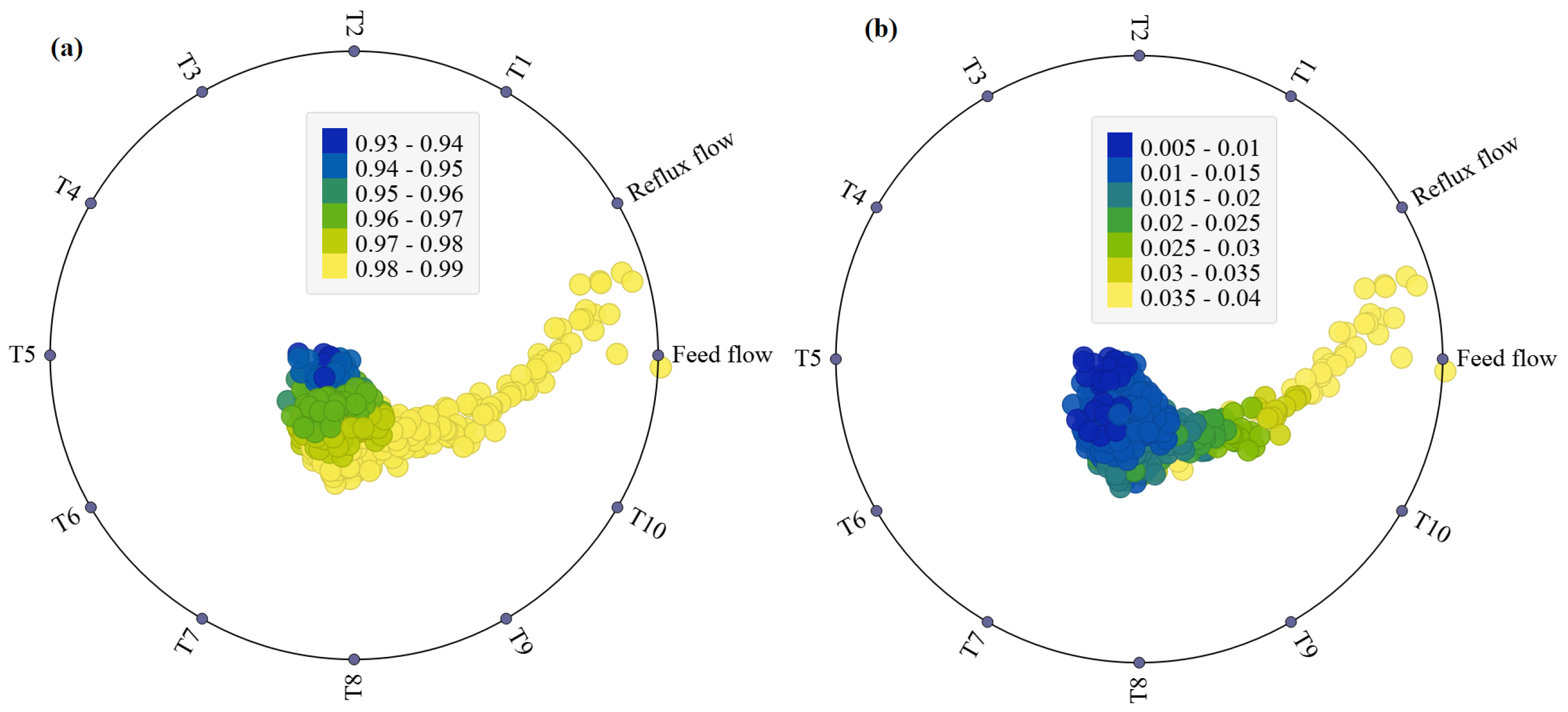
Figure 5a,b, RadViz is utilized to visually represent the relationships between various factors and the concentrations of ‘Propane’ and ‘Isobutene’ in the distillation column (DC). By examining the positioning of points and the density of lines, one can interpret how changes in different factors correspond to variations in the concentrations of these key components. RadViz, short for Radial Visualization, is a data visualization technique designed to understand the influence of multiple variables on a target variable [53]. The visualization is presented in a circular layout, where each variable is represented as a point on the circle’s circumference. The target variable is placed at the center of the circle. For each data point, the variables’ values determine its position along the circumference. The closer a point is to a particular variable, the higher the variable’s value for that specific data point. From Figure 5b, the RadViz plot reveals distinctive patterns in the impact of various factors on the concentration of Propane in the distillation column. Notably, Reflux and feed flow exhibit a significant influence, indicating their pivotal roles in determining Propane levels. Additionally, the temperatures T8, T9, and T10 also contribute substantially to the variation in Propane concentrations. The proximity of data points to these factors on the RadViz plot signifies their heightened impact, emphasizing the importance of monitoring and controlling Reflux, feed flow, and specific temperature variables for effectively managing Propane levels in the distillation column. From Figure 5b, the RadViz plot reveals that Reflux, feed flow, and temperatures T8, T9, and T10 notably influence Isobutene concentration. Efficient control and monitoring of these factors are crucial for managing Isobutene levels in the distillation column.
In this analysis, the dataset is divided into two sets: training (fault-free)data and testing data, each comprising 2048 data points. The training data is utilized to build both PCA and MPCA models independently. For a fair comparison, both models are constructed with 8 PCs. The optimal decomposition depths for the data are identified as 3 and 4 for signal-to-noise ratio (SNR) values of 15 and 5, respectively. This is illustrated in Figure 6.
To evaluate the fault detection performance of the PCA and MPCA models, bias, intermittent, and drift faults are considered in a simulated DC process. These faults in this analysis are assessed under different SNR scenarios (SNR = 15 and SNR = 5), providing insights into the models’ ability to detect and respond to different types of fault in varying noise levels.
  • Bias fault: A bias fault involves a constant offset in the readings of a particular sensor or variable. In this scenario, a 7% bias fault is introduced into temperature variable 5 from sampling time instant 250 until the end of the testing data. Introducing this fault in temperature variable 5 implies a persistent distortion in the measurements of this specific temperature parameter. This distortion persists throughout the latter part of the testing data, affecting the accuracy of the readings.
  • Drift fault: A drift fault signifies a gradual change or drift in the sensor readings over time. In this scenario, a drift sensor fault with a slope of 0.01 is introduced into temperature variable 1 during the same time frame. This introduced drift on testing data implies a continuous and gradual shift in the measurements of this temperature parameter. Such a fault can mimic the effect of changing conditions in the distillation column, potentially impacting process control.
  • Intermittent fault: An intermittent fault involves sporadic variations or disruptions in sensor readings. In this scenario, intermittent faults having a small magnitude with 8% of the total variation are inserted in the concentration variable of the bottom stream between the sampling time instants [100, 200] and [350, 450], respectively. Monitoring intermittent faults is crucial for capturing irregular disturbances in the system.
Understanding and addressing these fault scenarios is vital for maintaining the reliability and efficiency of distillation columns, as faults can impact the accuracy of sensor readings and, consequently, the control and optimization of the distillation process.
For visual representation,
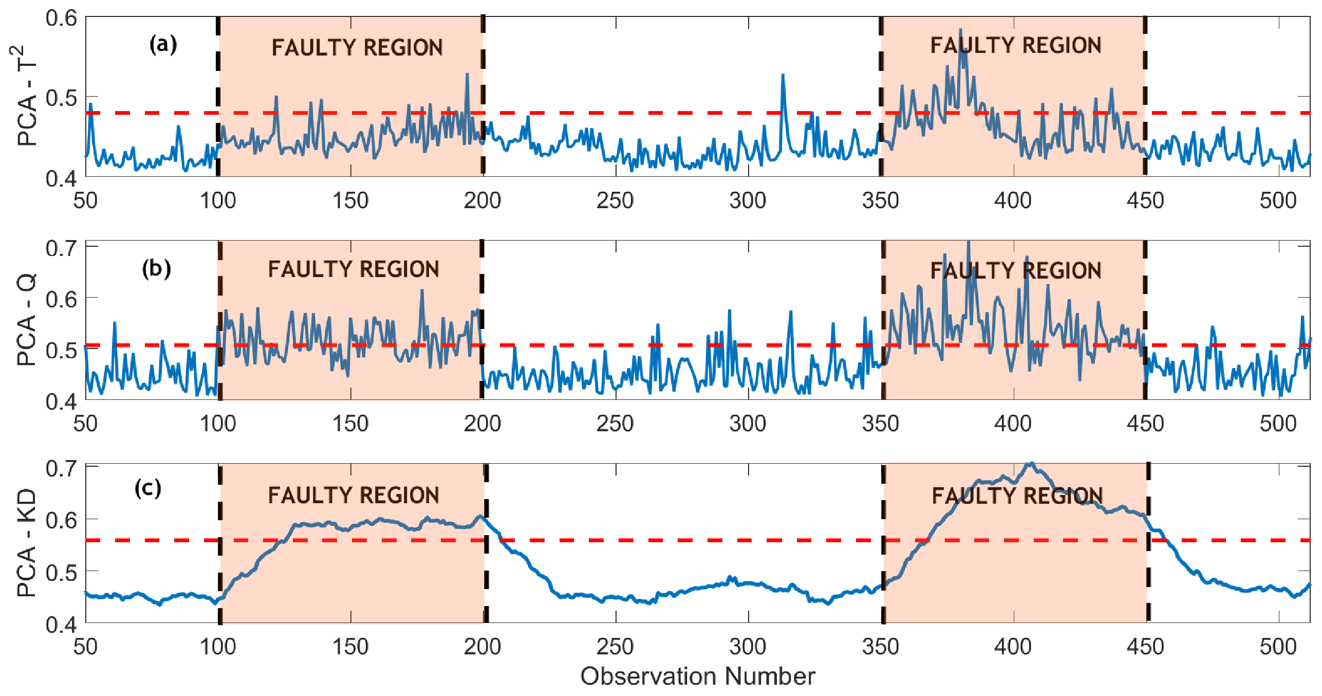
 Figure 7 and Figure 8 display the monitoring of an intermittent fault using PCA-based and MPCA-based methods under a Signal-to-Noise Ratio (SNR) of 15. In Figure 7a, the PCA- T 2 method exhibits shortcomings in detecting the intermittent fault, whereas the PCA-SPE method partially captures the fault but demonstrates some missed detections (Figure 7b). Notably, the PCA-KD scheme, illustrated in 
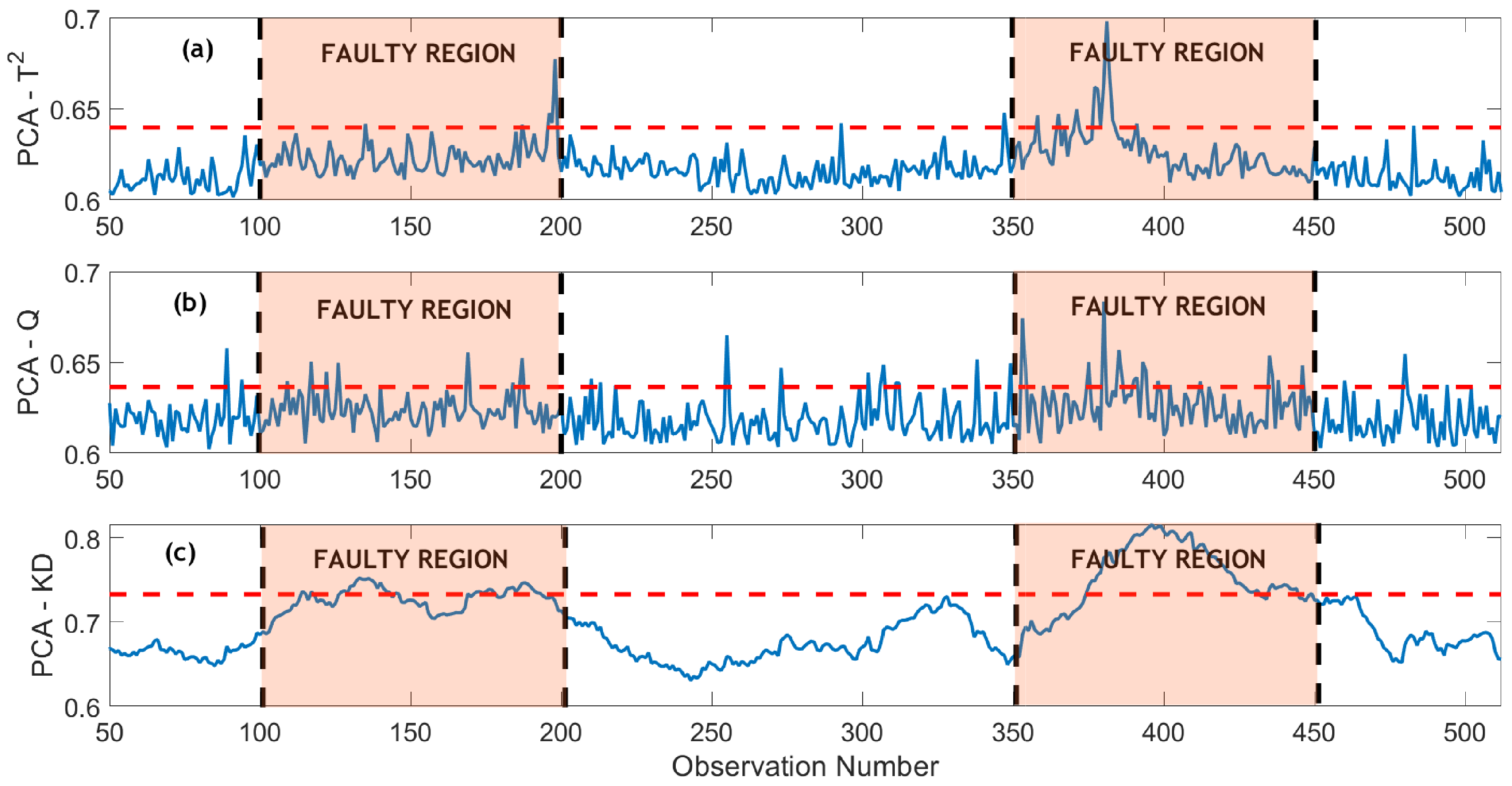
Figure 7c, shows improved fault detection compared to conventional methods but still exhibits some missed detections. In contrast, the wavelet-based methods outperform conventional methods in monitoring capabilities. The MPCA- T 2 and MPCA-SPE schemes show enhanced fault detection compared to PCA- T 2 and PCA-SPE methods, albeit with some missed detections and false alarms (Figure 8a–c). Remarkably, the proposed MPCA-KD scheme achieves accurate fault detection without missed detections or false alarms, providing a distinct advantage (Figure 8c). The superior performance of the MPCA-KD approach in fault detection can be attributed to its unique combination of multiscale MPCA with the KD scheme. The MSPCA-KD method excels in capturing critical details in the data by utilizing wavelet-based multiscale representation, which enhances its sensitivity to intermittent faults. The incorporation of KD, a distribution-based monitoring scheme, allows for a more nuanced comparison of data segments, contributing to improved fault detection. This underscores the effectiveness of the MPCA-KD approach in fault detection under conditions of intermittent faults and noise.
The evaluation of PCA and MPCA-based methods for monitoring three types of faults in the DC process has been conducted using several statistical metrics, namely, False Detection Rate (FDR), False Alarm Rate (FAR), Precision, and F1-score. Table 1 presents a comprehensive summary of the fault detection performance under an SNR of 15. For the bias fault, PCA-KD exhibited a high FDR of 82.06%, indicating a considerable proportion of false detections. On the other hand, MSPCA-KD demonstrated 100% FDR, implying a complete detection of the bias fault without false alarm (FAR = 0). MPCA-KD also achieved a perfect Precision and F1-score, suggesting superior accuracy in detecting the bias fault compared to other methods. In the case of intermittent faults, MSPCA-KD outperformed other methods with a 100% Precision and F1-score. Despite a relatively high FDR of 87.50%, PCA-KD showed moderate fault detection capabilities. MSPCA-Q exhibited higher FDR value with FDR 97%, indicating some trade-off between precision and recall in detecting intermittent faults. For drift faults, all methods demonstrated impressive fault detection performance, achieving 100% Precision and F1-score. MSPCA-Q and MSPCA-KD displayed slightly higher FDR values of 90.85 and 96.12, respectively and without false alarms. In summary, MPCA-KD consistently demonstrated superior fault detection accuracy across all fault types, emphasizing its effectiveness in monitoring complex systems like the distillation column process under an SNR of 15. The multiscale representation helps in efficiently extracting relevant features from the data, and the KD scheme further refines the detection process. This combination proves advantageous, especially in scenarios involving intermittent faults and noise, showcasing the effectiveness of the proposed MPCA-KD approach in enhancing fault detection reliability.
The monitoring of an intermittent fault under a high noise scenario (SNR = 5) is depicted in Figure 9 and Figure 10. In such conditions, where the SNR is low, distinguishing relevant signal variations from background noise becomes particularly challenging. The increased noise levels introduce complexities in fault detection, as the higher degree of random variations can obscure fault-related patterns. Conventional PCA-based methods struggle in the presence of substantial noise, failing to accurately identify the fault due to the masking effect of noise on important information. In comparison, the M S P C A T 2 and MSPCA-SPE schemes exhibit improved performance compared to PCA-based methods, providing partial detection of the fault. However, they still face challenges in achieving precise detection due to the influence of noise. Importantly, the proposed MSPCA-KD approach stands out in this high noise scenario. Despite the considerable noise present in the data, MSPCA-KD demonstrates robust fault detection capabilities. The method is able to discern the fault effectively, showcasing a smooth and accurate detection profile. This resilience to noise and ability to maintain a high level of precision in fault detection underscore the superiority of the MSPCA-KD approach in challenging and noisy environments. Overall, the results highlight the significance of the proposed method, especially in real-world scenarios where noise is inevitable. MSPCA-KD’s capacity to perform through high noise levels and deliver precise fault detection positions it as a valuable tool for monitoring complex systems in practical applications where noisy conditions are prevalent.
Table 2 provides an insightful overview of the fault detection performance of PCA and MPCA-based monitoring methods in the distillation column process under an SNR of 5. For the bias fault, PCA-KD exhibited a high FDR of 71.09%, indicating a significant proportion of false detections. MPCA-KD, while achieving 93.51% FDR, demonstrated superior fault detection capabilities compared to PCA-KD. MPCA-KD also achieved 100% Precision, suggesting precise detection of bias faults with no false alarms. The F1-score of MPCA-KD (87.60%) surpassed other methods, emphasizing its balanced performance in terms of precision and recall. Concerning intermittent faults, MPCA-KD outperformed other methods, achieving 98.75% FDR. Although PCA-KD demonstrated a lower FDR of 57.50%, MPCA-KD showcased superior fault detection accuracy with 100% Precision. This implies that MPCA-KD can accurately detect intermittent faults with minimal false positives. For drift faults, all methods demonstrated commendable fault detection performance, achieving 100% Precision and high F1-scores. PCA-KD and MPCA-KD displayed slightly higher FDR values, indicating a marginally increased rate of false detections compared to other methods. In summary, MPCA-KD consistently demonstrated superior fault detection accuracy across all fault types under an SNR of 5, further highlighting its effectiveness in monitoring the distillation column process in noisy conditions. The balanced performance of MPCA-KD, particularly in terms of Precision and FDR, makes it a robust choice for fault detection in complex systems with lower SNR.
The detection time ratio (DTR) of different methods in monitoring of three faults is highlighted in Table 3. For bias and intermittent faults, it may be observed that the proposed MSPCA-KD based FD strategy has a slightly higher value of DTR. Since the KD statistic is computed in a moving window, the proposed FD strategy tends to have a higher DTR value. Despite this, the proposed strategy has minimum missed detections and no false alarms. However, in case of drift fault, the proposed FD strategy has a slightly better DTR value. Overall, the superior performance of MPCA-KD, especially in fault detection scenarios with an SNR of 5, can be attributed to the MPCA and the KD scheme. PCA incorporates wavelet-based multiscale filtering, allowing the model to efficiently handle complex datasets with variations at multiple scales. This ensures that relevant features are retained while filtering out noise and irrelevant details, enhancing the model’s robustness. The use of KD as a statistical metric in the monitoring scheme enhances the model’s sensitivity to variations in data distributions. Essentially, MPCA-KD utilizes a distribution-based monitoring scheme, allowing it to compare segments of two distributions. This enables the model to capture critical details in the data, making it particularly effective in identifying anomalies and deviations associated with faults. The MPCA-KD approach employs nonparametric thresholding through kernel density estimation (KDE). This allows for a more flexible and adaptive determination of detection thresholds, accommodating variations in the data distribution without relying on strict assumptions.

3.2. Monitoring Faults in CSTR Process

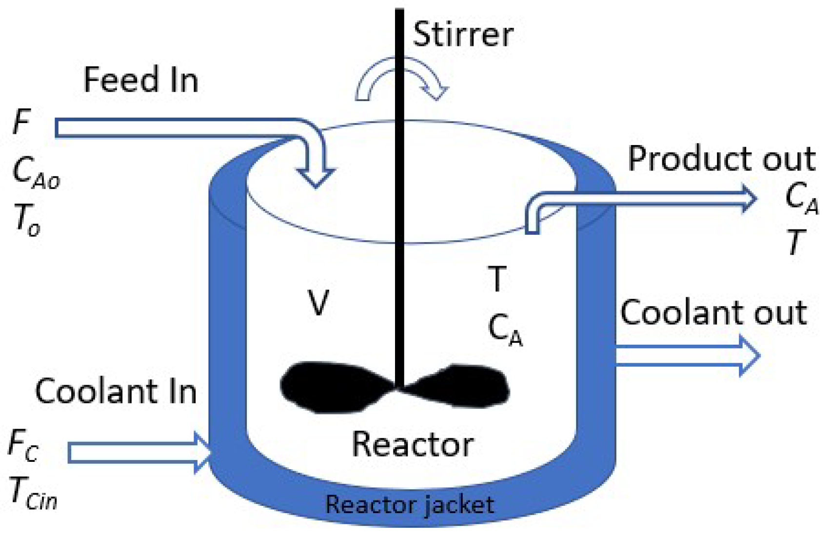
The experiment employs a nonlinear continuous stirred tank reactor (CSTR) setup to assess the efficacy of the proposed fault detection method. In a CSTR, reactants are introduced into the tank, and a stirrer mixes them to produce the desired product [54]. Numerous studies have employed different configurations of CSTRs to evaluate the efficacy of fault detection methodologies [55,56,57]. The CSTR process is characterized by a non-isothermal and irreversible first-order reaction [58]. Analyzing the proposed fault detection scheme’s performance in this particular CSTR setup offers valuable insights into its potential applications and effectiveness in real-world scenarios. The nonlinearity and dynamic nature of CSTR processes make them challenging for fault detection, making this evaluation particularly relevant for assessing the method’s robustness and applicability in complex and dynamic systems.
The discussed process involves a chemical reaction where species A undergoes a reaction to produce the desired product, B (i.e., A B ).
A B
Figure 11 illustrates the configuration of the Continuous Stirred Tank Reactor (CSTR) process. The reaction is highly exothermic, necessitating using the jacket’s fluid to cool the reactor. Precise regulation of the feed and coolant flow rates ensures the attainment of the desired product concentration, B. The reaction mechanism is described by Equation (20). By formulating component balance and energy balance equations for the reactor system, a set of Ordinary Differential Equations (ODEs) is derived, as presented in (21) through (23).
d C A d t = F V ( C A o C A ) k o e E / R T C A
d T d t = F V ( T o T ) + Δ H r ρ c p k o e E / R T C A Q V ρ c p
Q = a F c b + 1 F c + a F c b 2 ρ c c p c ( T c T c i n )
It is crucial to emphasize that the model relies on various parameters, outlined in Table 4. These parameters hold a pivotal role in determining the behavior of the reactor system. Consequently, comprehending the significance of each parameter and its influence on the system is essential for process optimization and achieving the target product concentration [59].
To generate data, the perturbation of feed stream and coolant flow rates around the steady state condition is carried out using a pseudo-random binary signal (PRBS) with frequency of [0 0.05 w N ], where w N = π / T represents the Nyquist frequency. This allows for the simulation of real-world scenarios where these variables may fluctuate due to external factors. It should also be noted that the variables C A o , T o and T c i n are treated as unmeasured disturbances. This means their dynamics are not directly measured or observed in the experiment. Instead, their behavior is governed by stochastic processes, which are used to model their potential effects on the system.
f 1 ( j ) = 0.1 1 0.9 z 1 d 1 ( j ) f 2 ( j ) = 0.3 1 0.7 z 1 d 2 ( j ) f 3 ( j ) = 0.3 1 0.7 z 1 d 3 ( j )
The { d 1 ( j ) } , { d 2 ( j ) } and { d 3 ( j ) } are white noise sequences that are having standard deviations of 0.5, 1 and 1 respectively.
Figure 12 depicts the heat map of the correlation matrix between the CSTR variables. A correlation coefficient of 0.822 between Reactor Temperature (T) and Reactor Concentration ( C A ) indicates a strong positive linear relationship between these two variables. In the context of a chemical reactor like the CSTR, the reactor’s temperature can influence the rate of chemical reactions. The positive correlation observed here might imply that higher temperatures within the reactor are associated with increased reactant concentrations. This relationship could be because many chemical reactions are temperature-dependent, and higher temperatures often lead to higher reaction rates. It’s important to note that correlation does not imply causation. While the correlation coefficient quantifies the strength and direction of a linear relationship, it doesn’t provide information about the underlying mechanisms or causative factors. Further analysis, experimentation, or domain knowledge would be needed to understand the specific reasons behind the observed correlation in the CSTR process.
A dataset of 1390 observations and seven variables is generated (Table 4). This data is partitioned into 745 samples each for training and testing purposes. PCA and MSPCA models are constructed, retaining five optimal PCs via the CPV method. For PCA-KD and MSPCA-KD strategies, KD computation employs a sliding window of 50. The optimal decomposition depth is determined to be 3 and 4 for SNR = 15 and SNR = 5, respectively. The analysis includes the monitoring of three faults in the CSTR process. In the first scenario, a bias fault, constituting 5% of the total variation, is introduced in the reactor temperature variable between sampling time instant 305 and the end of the testing data. In the second scenario, an intermittent fault with a magnitude of 5% of the total variation is inserted in the reactor concentration variable during two intervals: [200, 300] and [500, 600], respectively. Finally, a drift sensor fault with a slope of 0.001 is injected into the reactor concentration variable from sampling time instant 295 until the end of the testing data.
Detecting the introduced faults in the CSTR process, including a bias fault in the reactor temperature variable, an intermittent fault in the reactor concentration, and a drift sensor fault in the reactor concentration, is crucial for ensuring the robustness and reliability of the chemical reaction. The impact of these faults can influence the overall efficiency, product quality, and safety of the reactor system, making their timely detection and diagnosis essential for optimal process control and performance.
To enhance clarity, a detailed analysis of monitoring a bias fault in both noisy scenarios (SNR = 15 and SNR = 5) is presented through result plots. Figure 13 and 
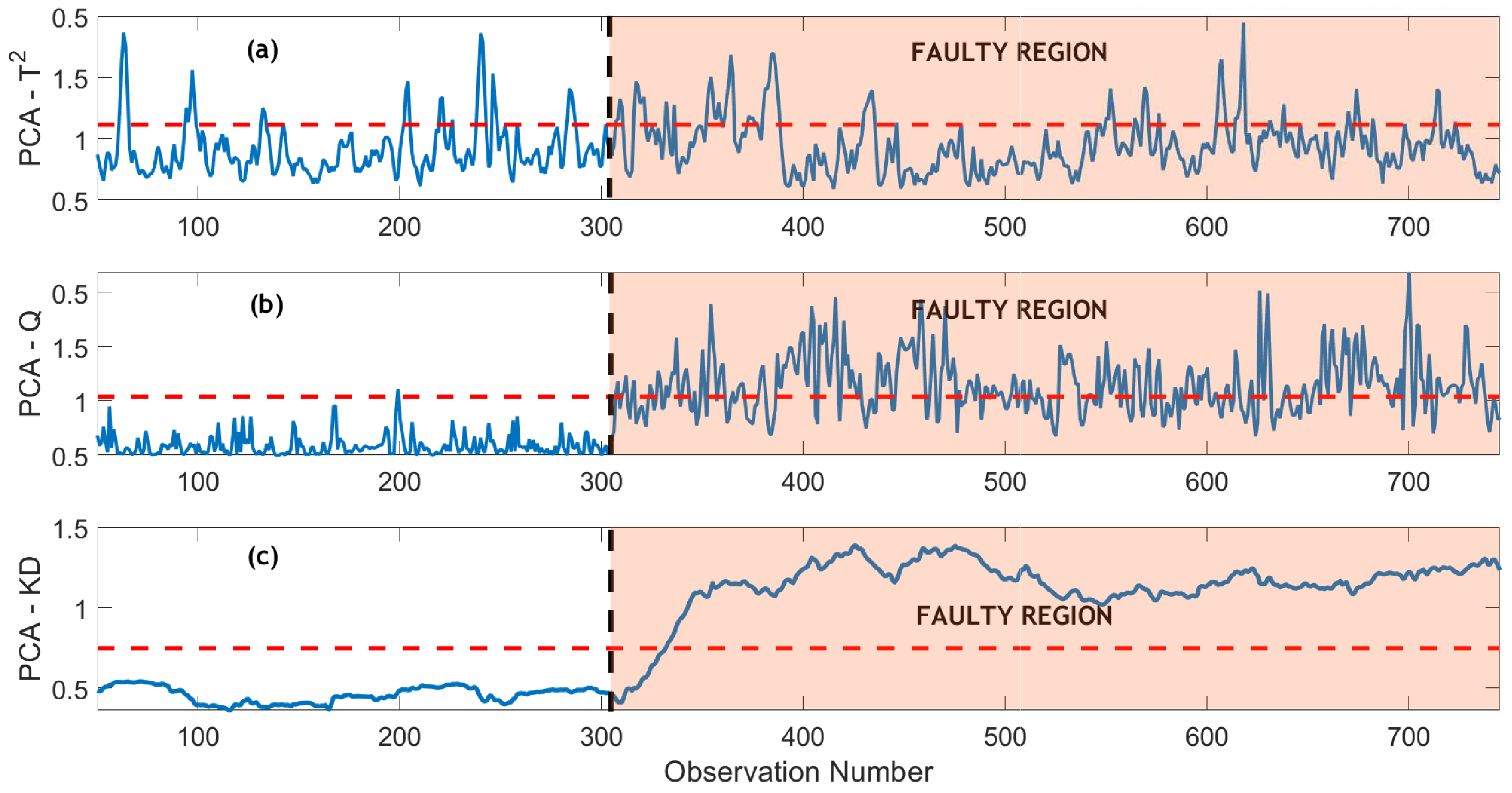
Figure 14 illustrate the monitoring of a bias fault by PCA and MPCA-based methods respectively in the SNR = 15 case. In Figure 13a, the T 2 indicator fails to identify the fault, as its statistical values remain below the reference threshold line within the fault region. Similarly, the PCA-Q strategy in Figure 13b also lacks effectiveness in detecting the bias fault, displaying multiple missed detections. This insensitivity to relatively small and moderate abnormal changes could stem from the decision statistics of T 2 and Q, which are designed solely based on the current observations without incorporating information from past data.
The performance exhibits a slight improvement with the MSPCA-Q strategy, attributed to the wavelet-based filtering (Figure 14b). Notably, the MSPCA-Q strategy successfully identifies the bias fault with few missed detections in the faulty region. In contrast, both the PCA-KD and MPCA-KD strategies outperform conventional PCA and MPCA-based methods in fault detection (Figure 13c and Figure 14c). The KD-based strategies provide smooth detection with minimal missed detections and zero false alarms. Importantly, the proposed MSPCA-KD strategy holds an advantage by detecting the fault with less delay compared to the PCA-KD strategy, showcasing its superiority.
Table 5 presents the performance of monitoring methods in detecting the three simulated faults in the CSTR process under an SNR of 15. In the case of a bias fault, PCA- T 2 shows a low detection rate of 12.45% and a low Precision, indicating frequent false alarms. PCA-Q exhibits a low FDR and a high FAR, making them unsuited in practice. For the Bias Fault, PCA-KD and MSPCA-KD exhibit superior FDR at 94.32% and 97.27%, respectively, indicating their efficacy in accurately identifying the bias fault. Concerning the intermittent fault, MSPCA-KD stands out with the highest FDR (95%) and zero false alarms, showcasing its ability to detect intermittent faults effectively (Table 5). MPCA-KD achieves perfect precision (100%) and F1-score, making it the most reliable for intermittent fault detection. This is attributed to the robustness provided by the wavelet-based filtering in MSPCA-KD. It is followed by MPCA-Q and PCA-KD, achieving an FDR of 79.5% and 75%, respectively. on the other hand, PCA- T 2 , PCA-Q, and MSPCA- T 2 exhibit high FAR and low FDR, indicating challenges in detecting drift faults accurately (Table 5). For the drift fault, PCA- T 2 and PCA-Q can recognize this fault but with many missed detections (i.e., FDR of 84.73% and 75.57%, respectively), indicating challenges in detecting drift faults accurately (Table 5). PCA-KD shows improvement in FDR (85.22 ) but still with several missed detections. MPCA- T 2 and MSPCA-Q offer better performance with improved FDR (88.02% and 90.85%) compared to PCA methods. MSPCA-KD outperforms other methods, achieving high FDR (96.12%), precision (100%), and F1-score (92.52%), making it the most effective in detecting drift faults (Table 5). MSPCA-KD’s incorporation of wavelet-based filtering contributes to its superior performance in minimizing false alarms while maintaining high precision, which is especially crucial in scenarios with SNR = 15.
In the subsequent analysis, the monitoring of the bias fault in the presence of heightened noise levels, characterized by an SNR of 5, is depicted in Figure 15 and Figure 16 respectively. Due to the significant noise level, the efficacy of PCA-based methods in detecting the bias fault is significantly compromised. Both the PCA- T 2 and PCA-Q schemes fail to identify the fault, underscoring their limitations in noisy conditions (Figure 15a,b). The PCA-KD strategy, while demonstrating improved detection compared to PCA- T 2 and PCA-Q, still exhibits a few missed detections within the fault region, as discerned in Figure 15c. In multi-scale-based methods, the MSPCA- T 2 strategy proves inefficient in detecting the bias fault amid the elevated noise environment (Figure 16a). The MSPCA-Q strategy performs better than PCA-based methods, yet it only achieves partial fault detection (Figure 16b). In contrast, the proposed MSPCA-KD-based strategy provides notable efficacy with a seamless detection of the bias fault within the fault region (Figure 16c). The method’s performance in the presence of substantial noise highlights its robustness and potential for reliable fault detection under challenging conditions.
Table 6 provides an insightful evaluation of various monitoring methods in detecting faults within the CSTR process under an SNR of 5. For the case of a bias fault, PCA-based methods exhibit limited effectiveness, particularly with PCA- T 2 displaying an FDR of 11.12%, indicating challenges in accurate fault detection. While PCA-Q demonstrates an improvement with a lower FDR of 32.95%, it still falls short of achieving optimal performance. PCA-KD, however, exhibits significant enhancements with an FDR of 71.73%, demonstrating its capability to identify bias faults more reliably. Multi-scale methods, specifically MPCA-KD, outperform other approaches in this scenario, achieving the highest FDR of 95.15%, indicating its robustness in detecting bias faults even in the presence of elevated noise. In the case of an intermittent fault, PCA-based methods face challenges, with PCA- T 2 and PCA-Q achieving FDRs of 13.25% and 48.00%, respectively. PCA-KD shows improvements with an FDR of 62.00%, but many missed detections remain. Multi-scale methods, especially MSPCA-KD, demonstrate superior fault detection capability with an FDR of 88.50%, showcasing its effectiveness in identifying intermittent faults with reduced missed detections. Considering drift faults, PCA-based methods present limitations, with PCA- T 2 and PCA-Q exhibiting FDRs of 44.11% and 68.67%, respectively. PCA-KD showcases improvement with an FDR of 71.39% but still has considerable missed detections. Multi-scale methods, notably MSPCA-KD, outperform other approaches with an FDR of 84.75%, indicating its ability to detect drift faults, but there is still room for improvement. In summary, under the SNR = 5 scenario, MSPCA-KD is the most effective method across all fault types, demonstrating superior fault detection rates, low false alarms, and high precision. The wavelet-based filtering in MPCA-KD contributes to its robustness, making it a reliable choice for fault detection in noisy environments.
The Table 7 provides the detection time ratio (DTR) of different methods in monitoring the three sensor faults of CSTR process. It may be noted that the proposed MSPCA-KD based FD strategy takes a small time to detect bias as well as intermittent faults and has a quicker detection for drift fault. It may be noted that the proposed MSPCA-KD strategy involves KD statistic which is computed in a moving window which contributes to small delay in computation. For a slowly varying drift fault, the MSPCA-KD strategy has a small advantage over the traditional methods as it has a better DTR value. The KD statistic excels at capturing subtle changes and patterns in the data, making it well-suited for fault detection, especially in situations where traditional methods may struggle. The utilization of wavelets with PCA model ensures that relevant features of the data are retained while filtering out noise and irrelevant details, enhancing the model’s robustness. This in turn enhanced the detection of different faults in the process.

4. Conclusions

In modern process plants, the impact of measurement noise on fault-detection methods has been a significant concern, leading to performance degradation. Among the available noise filtering methods, the integration of a multi-scale filtering scheme using wavelets with the PCA strategy has proven valuable, leveraging its capability to capture information across time-frequency scales. This work introduces a novel approach, the MSPCA-based fault detection strategy, which further enhances detection efficiency by incorporating the Kantorovich distance (KD)-based statistical indicators. Specifically, the MPCA-KD strategy evaluates MPCA residuals for fault detection, employing a non-parametric Kernel Density Estimation (KDE) scheme to compute the decision threshold. The optimal depth of decomposition is determined by assessing the PCA model at each level, selecting the level that minimizes the Mean Squared Error (MSE) of the model prediction. The proposed MPCA-KD strategy is assessed through two case studies: the simulated DC and CSTR processes. Results from both case studies consistently demonstrate the superiority of multi-scale methods over conventional ones, particularly for bias, intermittent, and drift faults. Notably, the MSPCA-KD strategy performs better by detecting each fault without generating false alarms and minimizing missed detections, even with substantial noise. This success can be attributed to the multi-scale decomposition using wavelets, which effectively filter noise and extract crucial process information, thereby enhancing fault detection capabilities. In conclusion, the proposed MPCA-KD fault detection strategy fulfills the essential criteria for a reliable fault monitoring scheme and represents a significant advancement in addressing the challenges posed by noise in industrial processes.
The current research successfully demonstrates the effectiveness of combining the KD approach and wavelet-based multi-scale filtering for fault detection in chemical processes. However, to further enhance the capabilities of fault detection systems, future work could explore integrating deep learning methods into this framework. Deep learning models, particularly recurrent neural networks (RNNs) and Long Short-Term Memory (LSTM) networks, have shown remarkable performance in capturing complex temporal patterns in sequential data [6]. The integration of these deep learning architectures can complement the existing KD and wavelet-based methods by automatically learning hierarchical representations from process data.

Author Contributions

K.R.K.: Writing—original draft, Formulation, Methodology, Software, Investigation; M.M.: Writing, Review and editing, Conceptualization, Formal analysis, Supervision, Validation; F.H.: Writing—Review and editing, Methodology, Supervision, Validation; A.K.V.: Visualization, Validation; Y.S.: Review and Editing, Visualization. All authors have read and agreed to the published version of the manuscript.

Funding

This research received no external funding.

Data Availability Statement

The data will be available on request.

Conflicts of Interest

The authors declare no conflict of interest.

References

  1. Kini, K.R.; Madakyaru, M.; Harrou, F.; Menon, M.K.; Sun, Y. Improved Fault Detection in Chemical Engineering Processes via Non-Parametric Kolmogorov–Smirnov-Based Monitoring Strategy. ChemEngineering 2024, 8, 1. [Google Scholar] [CrossRef]
  2. Memarian, A.; Raveendran, R.; Huang, B. Robust multi-mode probabilistic slow feature analysis with application to fault detection. J. Process. Control 2023, 132, 103130. [Google Scholar] [CrossRef]
  3. Park, Y.J.; Fan, S.K.S.; Hsu, C.Y. A Review on Fault Detection and Process Diagnostics in Industrial Processes. Processes 2020, 8, 1123. [Google Scholar] [CrossRef]
  4. Venkatasubramanian, V.; Rengaswamy, R.; Kavuri, S.N.; Yin, K. A review of process fault detection and diagnosis part 1: Quantitative model based methods. Comput. Chem. Eng. 2003, 27, 293–311. [Google Scholar] [CrossRef]
  5. Md Nor, N.; Che Hassan, C.R.; Hussain, M.A. A review of data-driven fault detection and diagnosis methods: Applications in chemical process systems. Rev. Chem. Eng. 2020, 36, 513–553. [Google Scholar] [CrossRef]
  6. Harrou, F.; Sun, Y.; Hering, A.S.; Madakyaru, M. Statistical Process Monitoring Using Advanced Data-Driven and Deep Learning Approaches: Theory and Practical Applications; Elsevier: Amsterdam, The Netherlands, 2020. [Google Scholar]
  7. Isermann, R. Model-based fault-detection and diagnosis–status and applications. Annu. Rev. Control 2005, 29, 71–85. [Google Scholar] [CrossRef]
  8. Yin, S.; Ding, S.X.; Xie, X.; Luo, H. A review on basic data-driven approaches for industrial process monitoring. IEEE Trans. Ind. Electron. 2014, 61, 6418–6428. [Google Scholar] [CrossRef]
  9. Montgomery, D.C. Introduction to Statistical Quality Control; John Wiley & Sons: Hoboken, NJ, USA, 2019. [Google Scholar]
  10. Bersimis, S.; Psarakis, S.; Panaretos, J. Multivariate statistical process control charts: An overview. Qual. Reliab. Eng. Int. 2007, 23, 517–543. [Google Scholar] [CrossRef]
  11. Ramos, M.; Ascencio, J.; Hinojosa, M.V.; Vera, F.; Ruiz, O.; Jimenez-Feijoó, M.I.; Galindo, P. Multivariate statistical process control methods for batch production: A review focused on applications. Prod. Manuf. Res. 2021, 9, 33–55. [Google Scholar] [CrossRef]
  12. Nassif, A.B.; Talib, M.A.; Nasir, Q.; Dakalbab, F.M. Machine learning for anomaly detection: A systematic review. IEEE Access 2021, 9, 78658–78700. [Google Scholar] [CrossRef]
  13. Pang, G.; Shen, C.; Cao, L.; Hengel, A.V.D. Deep learning for anomaly detection: A review. ACM Comput. Surv. (CSUR) 2021, 54, 1–38. [Google Scholar] [CrossRef]
  14. Joe Qin, S. Statistical process monitoring: Basics and beyond. J. Chemom. A J. Chemom. Soc. 2003, 17, 480–502. [Google Scholar] [CrossRef]
  15. Harrou, F.; Nounou, M.N.; Nounou, H.N.; Madakyaru, M. Statistical fault detection using PCA-based GLR hypothesis testing. J. Loss Prev. Process. Ind. 2013, 26, 129–139. [Google Scholar] [CrossRef]
  16. Harrou, F.; Kini, K.R.; Madakyaru, M.; Sun, Y. Uncovering sensor faults in wind turbines: An improved multivariate statistical approach for condition monitoring using SCADA data. Sustain. Energy Grids Netw. 2023, 35, 101126. [Google Scholar] [CrossRef]
  17. Lee, J.M.; Qin, S.J.; Lee, I.B. Fault detection and diagnosis based on modified independent component analysis. AIChE J. 2006, 52, 3501–3514. [Google Scholar] [CrossRef]
  18. Zhong, B.; Wang, J.; Zhou, J.; Wu, H.; Jin, Q. Quality-related statistical process monitoring method based on global and local partial least-squares projection. Ind. Eng. Chem. Res. 2016, 55, 1609–1622. [Google Scholar] [CrossRef]
  19. Harrou, F.; Sun, Y.; Madakyaru, M.; Bouyedou, B. An improved multivariate chart using partial least squares with continuous ranked probability score. IEEE Sens. J. 2018, 18, 6715–6726. [Google Scholar] [CrossRef]
  20. Harrou, F.; Sun, Y.; Hering, A.S.; Madakyaru, M.; Dairi, A. Unsupervised Recurrent Deep Learning Scheme for Process Monitoring; Elsevier BV: Amsterdam, The Netherlands, 2021. [Google Scholar]
  21. Hu, Z.; Zhao, H.; Peng, J. Low-rank reconstruction-based autoencoder for robust fault detection. Control. Eng. Pract. 2022, 123, 105156. [Google Scholar] [CrossRef]
  22. Yu, W.; Wu, M.; Huang, B.; Lu, C. A generalized probabilistic monitoring model with both random and sequential data. Automatica 2022, 144, 110468. [Google Scholar] [CrossRef]
  23. Yu, W.; Zhao, C. Robust monitoring and fault isolation of nonlinear industrial processes using denoising autoencoder and elastic net. IEEE Trans. Control. Syst. Technol. 2019, 28, 1083–1091. [Google Scholar] [CrossRef]
  24. Tang, P.; Peng, K.; Zhang, K.; Chen, Z.; Yang, X.; Li, L. A deep belief network-based fault detection method for nonlinear processes. IFAC-PapersOnLine 2018, 51, 9–14. [Google Scholar] [CrossRef]
  25. Yu, W.; Zhao, C.; Huang, B. MoniNet with concurrent analytics of temporal and spatial information for fault detection in industrial processes. IEEE Trans. Cybern. 2021, 52, 8340–8351. [Google Scholar] [CrossRef]
  26. Zhang, Y.; Ma, C. Fault diagnosis of nonlinear processes using multiscale KPCA and multiscale KPLS. Chem. Eng. Sci. 2011, 66, 64–72. [Google Scholar] [CrossRef]
  27. Zhang, Y.; Hu, Z. Multivariate process monitoring and analysis based on multi-scale KPLS. Chem. Eng. Res. Des. 2011, 89, 2667–2678. [Google Scholar] [CrossRef]
  28. Harrou, F.; Sun, Y.; Hering, A.S.; Madakyaru, M.; Dairi, A. Multiscale latent variable regression-based process monitoring methods. In Statistical Process Monitoring Using Advanced Data-Driven and Deep Learning Approaches; Elsevier: Amsterdam, The Netherlands, 2021; pp. 155–191. [Google Scholar]
  29. Bakshi, B.R. Multiscale analysis and modeling using wavelets. J. Chemom. 1999, 13, 415–434. [Google Scholar] [CrossRef]
  30. Palavajjhala, S.; Motard, R.L.; Joseph, B. Process identification using discrete wavelet transforms: Design of prefilters. AIChE J. 1996, 42, 777–790. [Google Scholar] [CrossRef]
  31. Aradhye, H.B.; Bakshi, B.R.; Strauss, R.A.; Davis, J.F. Multiscale SPC using wavelets: Theoretical analysis and properties. AIChE J. 2003, 49, 939–958. [Google Scholar] [CrossRef]
  32. Guo, H.; Guo, H.; Guo, H.; Guo, H.; Paynabar, K.; Jin, J. Multiscale monitoring of autocorrelated processes using wavelets analysis. IIE Trans. 2012, 44, 312–326. [Google Scholar] [CrossRef]
  33. Yellapu, V.S.; Vajpayee, V.; Tiwari, A.P.; Tiwari, A.P.; Tiwari, A.P. Online Fault Detection and Isolation in Advanced Heavy Water Reactor Using Multiscale Principal Component Analysis. IEEE Trans. Nucl. Sci. 2019, 66, 1790–1803. [Google Scholar] [CrossRef]
  34. Chanerley, A.; Alexander, N. Correcting data from an unknown accelerometer using recursive least squares and wavelet de-noising. Comput. Struct. 2007, 85, 1679–1692. [Google Scholar] [CrossRef]
  35. Maulud, A.; Wang, D.; Romagnoli, J. A multi-scale orthogonal nonlinear strategy for multi-variate statistical process monitoring. J. Process. Control 2006, 16, 671–683. [Google Scholar] [CrossRef]
  36. Teppola, P.; Minkkinen, P. Wavelet–PLS regression models for both exploratory data analysis and process monitoring. J. Chemom. 2000, 14, 383–399. [Google Scholar] [CrossRef]
  37. Isermann, R.; Isermann, R. Fault detection with principal component analysis (PCA). In Fault-Diagnosis Systems: An Introduction from Fault Detection to Fault Tolerance; Springer: Berlin/Heidelberg, Germany, 2006; pp. 267–278. [Google Scholar]
  38. Ralston, P.; DePuy, G.; Graham, J.H. Computer-based monitoring and fault diagnosis: A chemical process case study. ISA Trans. 2001, 40, 85–98. [Google Scholar] [CrossRef]
  39. MacGregor, J. Multivariate statistical methods for monitoring large data sets from chemical processes. In Proceedings of the AIChE Meeting, San Francisco, CA, USA, 5–10 November 1989. [Google Scholar]
  40. Zhu, M.; Ghodsi, A. Automatic dimensionality selection from the scree plot via the use of profile likelihood. Comput. Stat. Data Anal. 2006, 51, 918–930. [Google Scholar] [CrossRef]
  41. Li, W.; Peng, M.; Wang, Q. Fault identification in PCA method during sensor condition monitoring in a nuclear power plant. Ann. Nucl. Energy 2018, 121, 135–145. [Google Scholar] [CrossRef]
  42. Tao, E.; Shen, W.; Liu, T.; Chen, X. Fault diagnosis based on PCA for sensors of laboratorial wastewater treatment process. Chemom. Intell. Lab. Syst. 2013, 128, 49–55. [Google Scholar] [CrossRef]
  43. Sanjula, K.; Zukiu, L. Change point and fault detection using Kantorovich Distance. J. Process. Control 2019, 80, 41–59. [Google Scholar]
  44. Kini, K.R.; Madakyaru, M. Improved Process Monitoring Scheme Using Multi-Scale Independent Component Analysis. Arab. J. Sci. Eng. 2022, 47, 5985–6000. [Google Scholar] [CrossRef]
  45. Zhou, S.; Sun, B.; Shi, J. An SPC monitoring system for cycle-based waveform signals using haar transform. IEEE Trans. Autom. Sci. Eng. 2006, 3, 60–72. [Google Scholar] [CrossRef]
  46. Lee, D.S.; Park, J.M.; Vanrolleghem, P.A. Adaptive multiscale principal component analysis for on-line monitoring of a sequencing batch reactor. J. Biotechnol. 2005, 516, 195–210. [Google Scholar] [CrossRef]
  47. Madakyaru, M.; Harrou, F.; Sun, Y. Improved data-based fault detection strategy and application to distillation columns. Process. Saf. Environ. Prot. 2017, 107, 22–34. [Google Scholar] [CrossRef]
  48. Donoho, D.L.; Johnstone, I.M.; Kerkyacharian, G.; Picard, D. Wavelet shrinkage: Asymptopia? J. R. Stat. Soc. Ser. B 1995, 57, 301–369. [Google Scholar] [CrossRef]
  49. Donoho, D.L.; Johnstone, I.M. Ideal spatial adaptation by wavelet shrinkage. Biometrika 1994, 81, 425–455. [Google Scholar] [CrossRef]
  50. Lee, H.W.; Lee, M.W.; Park, J.M. Multi-scale extension of PLS algorithm for advanced on-line process monitoring. Chemom. Intell. Lab. Syst. 2009, 98, 201–212. [Google Scholar] [CrossRef]
  51. Taqvi, S.A.T.S.A.; Tufa, L.D.; Zabiri, H.; Maulud, A.S.; Uddin, F. Multiple Fault Diagnosis in Distillation Column Using Multikernel Support Vector Machine. Ind. Eng. Chem. Res. 2018, 57, 14689–14706. [Google Scholar] [CrossRef]
  52. Harrou, F.; Sun, Y.; Madakyaru, M. Kullback-leibler distance-based enhanced detection of incipient anomalies. J. Loss Prev. Process. Ind. 2016, 44, 73–87. [Google Scholar] [CrossRef]
  53. Abraham, Y.; Gerrits, B.; Ludwig, M.G.; Rebhan, M.; Gubser Keller, C. Exploring Glucocorticoid Receptor Agonists Mechanism of Action Through Mass Cytometry and Radial Visualizations. Cytom. Part B Clin. Cytom. 2017, 92, 42–56. [Google Scholar] [CrossRef]
  54. Pilario, K.E.S.; Cao, Y. Canonical variate dissimilarity analysis for process incipient fault detection. IEEE Trans. Ind. Inform. 2018, 14, 5308–5315. [Google Scholar] [CrossRef]
  55. Choi, S.W.; Lee, C.; Lee, J.M.; Park, J.H.; Lee, I.B. Fault detection and identification of nonlinear processes based on kernel PCA. Chemom. Intell. Lab. Syst. 2005, 75, 55–67. [Google Scholar] [CrossRef]
  56. Pilario, K.E.; Cao, Y. Process incipient fault detection using canonical variate analysis. In Proceedings of the 2017 23rd International Conference on Automation and Computing (ICAC), Huddersfield, UK, 7–8 September 2017; pp. 1–6. [Google Scholar]
  57. Juricek, B.C.; Seborg, D.E.; Larimore, W.E. Fault detection using canonical variate analysis. Ind. Eng. Chem. Res. 2004, 43, 458–474. [Google Scholar] [CrossRef]
  58. Yang, X.; Wei, Q. Adaptive Critic Designs for Optimal Event-Driven Control of a CSTR System. IEEE Trans. Ind. Inform. 2021, 17, 484–493. [Google Scholar] [CrossRef]
  59. Jafari, N.; Lopes, A.M. Fault Detection and Identification with Kernel Principal Component Analysis and Long Short-Term Memory Artificial Neural Network Combined Method. Axioms 2023, 12, 583. [Google Scholar] [CrossRef]
Figure 1. Multiscale decomposition of a heavy-sine signal using Haar wavelet.
Chemengineering 08 00045 g001
Figure 2. Multiscale PCA-KD based fault detection strategy.
Chemengineering 08 00045 g002
Figure 3. A schematic overview of the distillation column process, highlighting structural components, RTD sensors, and the entry conditions for a binary mixture of propane and isobutene.
Chemengineering 08 00045 g003
Figure 4. Correlation matrix heatmap depicting the Pearson correlation among variables in the fault-free distillation column dataset.
Chemengineering 08 00045 g004
Figure 5. RadViz visualization illustrating the influence of different factors on (a) ‘Propane’ and (b) ‘Isobutene’ concentrations in the distillation column. Each point on the circular plot represents a data point, and the positioning of points along the circumference reflects the values of various factor.
Chemengineering 08 00045 g005
Figure 6. Calculation of decomposition depth for (a) SNR = 15 and (b) SNR = 5.
Chemengineering 08 00045 g006
Figure 7. Intermittent fault monitoring in the DC process by PCA based methods under SNR level of 15: (a) PCA- T 2 , (b) PCA-Q, (c) PCA-KD (Red line indicates significance threshold).
Chemengineering 08 00045 g007
Figure 8. Intermittent fault monitoring in the DC process by MSPCA based methods under SNR level of 15: (a) MSPCA- T 2 , (b) MSPCA-Q, (c) MSPCA-KD (Red line indicates significance threshold).
Chemengineering 08 00045 g008
Figure 9. Intermittent fault monitoring in the DC process by PCA based methods under SNR level of 5: (a) PCA- T 2 , (b) PCA-Q, (c) PCA-KD (Red line indicates significance threshold).
Chemengineering 08 00045 g009
Figure 10. Intermittent fault monitoring in the DC process by MSPCA based methods under SNR level of 5: (a) MSPCA- T 2 , (b) MSPCA-Q, (c) MSPCA-KD (Red line indicates significance threshold).
Chemengineering 08 00045 g010
Figure 11. A schematic of distillation column process.
Chemengineering 08 00045 g011
Figure 12. Correlation matrix of the fault-free CSTR data.
Chemengineering 08 00045 g012
Figure 13. Bias fault monitoring by PCA based methods in the CSTR process under SNR level of 15: (a) PCA- T 2 , (b) PCA-Q, (c) PCA-KD (Red line indicates significance threshold).
Chemengineering 08 00045 g013
Figure 14. Bias fault monitoring by MPCA based methods in the CSTR process under SNR level of 15: (a) MSPCA- T 2 , (b) MSPCA-Q, and (c) MSPCA-KD (Red line indicates significance threshold).
Chemengineering 08 00045 g014
Figure 15. Bias fault monitoring by PCA based methods in the CSTR process under SNR level of 5: (a) PCA- T 2 , (b) PCA-Q, (c) PCA-KD (Red line indicates significance threshold).
Chemengineering 08 00045 g015
Figure 16. Bias fault monitoring by MPCA based methods in the CSTR process under SNR level of 5: (a) MSPCA- T 2 , (b) MSPCA-Q, and (c) MSPCA-KD. (Red line indicates significance threshold).
Chemengineering 08 00045 g016
Table 1. Fault detection performance of PCA and MSPCA-based monitoring methods in the distillation column process under an SNR of 15.
FaultIndexPCA- T 2 PCA-QPCA-KDMPCA- T 2 MPCA-QMPCA-KD
BiasFDR46.1858.4982.0694.5683.59100.00
FAR0.807.600.000.041.600.00
Precision98.3788.95100.0099.5998.20100.00
F1-score63.0966.2790.1497.0990.70100.00
IntermFDR22.5060.0087.5095.0097.00100.00
FAR0.006.410.003.5211.000.00
Precision100.0095.23100.0085.4685.46100.00
F1-score36.9875.0393.3094.5091.09100.00
DriftFDR84.7375.5785.2288.0290.8596.12
FAR0.000.000.000.000.000.00
Precision100.00100.00100.00100.00100.00100.00
F1-score91.7386.0892.0293.6295.2098.02
Table 2. Fault detection performance of PCA and MSPCA-based monitoring methods in the distillation column process under an SNR of 5.
FaultIndexPCA- T 2 PCA-QPCA-KDMPCA- T 2 MPCA-QMPCA-KD
BiasFDR10.7851.3871.0920.9471.7693.51
FAR1.208.400.000.404.400.00
Precision86.7388.95100.0099.2394.47100.00
F1-score19.5965.0587.6034.3681.6896.64
IntermFDR8.4115.5057.5038.0075.5098.75
FAR0.008.000.005.286.420.00
Precision100.0055.30100.0082.1088.40100.00
F1-score16.6624.7473.0152.0081.4299.31
DriftFDR63.3646.5665.7580.1583.2186.50
FAR0.000.400.000.000.000.00
Precision100.0099.17100.00100.00100.00100.00
F1-score77.5762.8279.3388.9888.8092.62
Table 3. DC process: Detection Time Ratio (DTR).
SNRFaultPCA- T 2 PCA-QPCA-KDMPCA- T 2 MPCA-QMPCA-KD
15Bias0.0030.0030.0940.0070.0010.038
Intermittent0.4500.0100.1100.0100.0100.060
Drift0.2290.2350.21750.1330.1140.076
5Bias0.4200.0380.1290.3120.0380.091
Intermittent0.6500.6750.1750.2500.0100.050
Drift0.3620.4270.3120.2290.1900.160
Table 4. Variables considered in CSTR process.
VariablesSymbolUnits
Reactor TemperatureTK
Reactor Concentration C A kmol/m3
Flow rate of feed streamFm3/min
Flow rate of coolant flow F c m3/min
Inlet concentration C A o kmol/m3
Inlet temperature of reactant A T o K
Inlet temperature of the coolant T c i n K
Table 5. Performance of monitoring methods in detecting faults in CSTR process for SNR = 15.
FaultIndexPCA- T 2 PCA-QPCA-KDMPCA- T 2 MPCA-QMPCA-KD
BiasFDR12.4540.3694.3225.1475.2397.27
FAR7.841.000.0010.751.640.00
Prec70.5198.38100.0077.0898.16100.00
F1-score21.3057.4297.0737.6284.9898.61
IntermFDR14.5055.5075.0016.5079.5095.00
FAR5.422.650.003.852.250.00
Prec50.0090.24100.0061.1192.44100.00
F1-score22.4868.8485.7126.1985.4597.43
DriftFDR50.7870.4473.1160.7275.2286.09
FAR8.151.000.006.780.000.00
Prec90.4099.06100.0093.20100.00100.00
F1-score65.1882.0984.4673.9985.8592.52
Table 6. Performance of monitoring methods in detecting faults in CSTR process for SNR = 5.
FaultIndexPCA- T 2 PCA-QPCA-KDMPCA- T 2 MPCA-QMPCA-KD
BiasFDR11.1232.9571.7318.8662.0595.15
FAR9.182.300.0010.431.000.00
Prec63.6395.39100.0072.1798.74100.00
F1-score19.1249.1183.5330.0076.1197.51
IntermFDR13.2548.0062.0013.0075.0088.50
FAR7.713.000.004.592.020.00
Prec38.9785.71100.0050.9093.16100.00
F1-score19.8661.8476.5421.0083.1894.00
DriftFDR44.1168.6771.3955.4573.1184.75
FAR5.410.000.006.450.000.00
Prec92.32100.00100.0092.93100.00100.00
F1-score59.4581.4283.3069.6384.4691.74
Table 7. CSTR process: Detection Time Ratio (DTR).
SNRFaultPCA- T 2 PCA-QPCA-KDMPCA- T 2 MPCA-QMPCA-KD
15Bias0.0250.0060.0790.0200.0050.054
Intermittent0.1400.0070.1800.2500.0070.100
Drift0.3110.2880.2660.3000.2330.155
5Bias0.0680.0560.1930.0310.0050.061
Intermittent0.1600.0070.2000.2800.0070.105
Drift0.3620.4270.3120.3510.2550.166
Disclaimer/Publisher’s Note: The statements, opinions and data contained in all publications are solely those of the individual author(s) and contributor(s) and not of MDPI and/or the editor(s). MDPI and/or the editor(s) disclaim responsibility for any injury to people or property resulting from any ideas, methods, instructions or products referred to in the content.

