
Lattice Boltzmann Simulation of Cavitating Flow in a Two-Dimensional Nozzle with Moving Needle Valve

1
School of Energy and Power Engineering, University of Shanghai for Science and Technology, Shanghai 200093, China
2
Shanghai Key Laboratory of Multiphase Flow and Heat Transfer in Power Engineering, Shanghai 200093, China
*
Author to whom correspondence should be addressed.
Processes 2024, 12(4), 813; https://0-doi-org.brum.beds.ac.uk/10.3390/pr12040813
Submission received: 5 March 2024
/
Revised: 13 April 2024
/
Accepted: 16 April 2024
/
Published: 18 April 2024
(This article belongs to the Section Advanced Digital and Other Processes)
Abstract
:A cascaded pseudo-potential lattice Boltzmann model and refilling algorithms for moving boundary treatment were used to simulate the large density ratio cavitating flow in a two-dimensional nozzle with the periodic motion of the needle valve. The relationships between density variation at the cavitation zone, the evolution of force acting on the lower boundary of the sack wall region, and the surface of the needle valve with time under different needle valve motion frequencies were obtained. The results indicate that the inception and evolution of cavitation mainly exist in the vicinity of the lower boundary of the sack wall region. The density at cavitation decreases by approximately three orders of magnitude, while the force on the lower boundary of the sack wall region decreases by about one order of magnitude. Since cavitation does not exist in the vicinity of the needle valve, the forces are mainly influenced by the periodic motion of the needle valve and do not change significantly. Changes in the frequency of needle valve motion affect the time taken for cavitation evolution to reach a relatively steady state but do not significantly affect the forces acting on the different components.
1. Introduction
Vapor–liquid phase change phenomena are ubiquitous in nature and human activities, arising from two key drivers: temperature gradients, which create evaporation or condensation, and pressure gradients, which lead to cavitation. In industrial processes, cavitation often accompanies moving solid boundaries, including valve spools, propellers, and other machinery. Examples include cavitation from spool movement in valves [1] or marine propeller rotation in ship propulsion systems.
As simple throttling valves with precise control, needle valves enable accessible flow regulation across agriculture, medicine, food, machinery, and beyond. Needles inject required engine fuel into the combustion chambers within the diesel nozzle. Needle valve motion greatly influences internal nozzle flow patterns and cavitation formation.
With the advancement of industrial technology and the increasing demand for precise control of fluids, research into the internal flow within nozzles has been continuously deepened. Researchers have conducted comprehensive studies of the fluid dynamics within nozzles through numerical simulations, experimental measurements, and theoretical analyses, focusing on issues such as cavitation formation and needle valve motion that impact the system. Guo et al. [2] developed a 3D computational fluid dynamics model to simulate swirling cavitation flows inside diesel engine nozzles, performing simulations to determine impacts on internal flow patterns and spray dynamics. Their results indicated that intensified inlet pressures progressively diminish the influence and intensity of swirling cavitation structures. Wei et al. [3] used high-speed microscopic imaging to conduct experiments on conical orifice nozzles. They discovered that fluctuation trends, such as pressure drop and fluctuation duration, can effectively respond to cavitation morphology. Based on the identification of the high and low frequencies of pressure fluctuations, these trends can theoretically support studies of cavitation characterization. Yang et al. [4] proposed a novel, non-invasive method of measuring needle valve motion to examine the effect of needle valve motion on the injector’s injection rate. The findings demonstrated that the injection rate is not linearly related to changes in the spool position and that the spool’s lifting speed varies as gas injection pressure changes. Huang et al. [5] investigated the kinematic characteristics of the needle valve in the nozzle and the liquid jet dynamics in the near-nozzle field using X-ray imaging over a more relaxed range of injection pulse durations. They concluded that the lack of needle valve lift would affect the momentum of the liquid jet during the injection pulse duration.
A review of the relevant literature reveals that the predominant approach to analyzing internal needle valve flow fields has entailed experimental methods and solving the Navier–Stokes equations based on assumptions of continuum fluid mechanics. However, over the last three decades, scholars have progressively developed mesoscopic computational methods founded on statistical mechanics, notably the lattice Boltzmann method (LBM). Owing to innate advantages for parallelization and resolving complex boundaries, LBM has attained widespread adoption for simulating phenomena such as multiphase flow [6], deformable fluid-filled bodies [7], fluid–structure interaction [8], Phase Change Material Energy Storage [9], fuel cells [10], acoustics [11], combustion applications [12], boiling, and evaporation [13].
Currently, the immersed boundary method and the refilling algorithms are the two main approaches to tackling the motion geometry problem of the LBM. The immersed boundary method was first proposed by Peskin [14], and its main idea is to perform calculations by applying a force field instead of a boundary. The refilling algorithms mainly initialize the “fresh” fluid nodes, which have been gradually promoted because of their significant advantage in improving computational stability. Current research indicates that five distinct variations of the refilling algorithms have been developed to date. The averaged extrapolation (AEP) method was proposed by Fang et al. [15] and primarily computes the mean extrapolation of the fresh fluid nodes’ distribution function without direction specification. Luo et al. [16] proposed two methods: the extrapolation (EP) method uses second-order extrapolation to treat the non-equilibrium distribution function (FNEQ) and the density of the fresh fluid nodes. In contrast, the equilibrium distribution function (FEQ) method assigns the flow field’s mean density and the moving geometry’s velocity to the fresh fluid nodes. First-order extrapolation is used to treat the FNEQ of the fresh fluid nodes in Caiazzo et al.’s [17] FEQ+FNEQ method, which is based on the FEQ method. On the other hand, Ansumali et al. [18] applied the Grad-type distribution function to initialize the fresh fluid nodes. After thoroughly comparing the five refilling algorithms, Tao et al. [19] concluded that the FEQ+FNEQ method offered a more thorough solution to the problem and more straightforward computational steps than other algorithms. For this reason, this method is also utilized in this paper to realize the treatment of moving geometry.
A variety of multiphase lattice Boltzmann models have emerged, including the color-gradient (R − K) model [20,21], the pseudo-potential model [22,23], the free energy model [24], and the phase field model [25,26]. The pseudo-potential model has emerged as the predominant approach for multiphase lattice Boltzmann modeling due to its computational efficiency and capacity to capture the motion of the phase interface freely. Based on the current literature, the application of the pseudo-potential model to investigate phase change issues related to cavitation predominantly focuses on two areas: cavitation bubbles and cavitating flows. In the study of cavitation bubbles, He et al. [27,28,29] utilized the multiple-relaxation-time (MRT) pseudo-potential lattice Boltzmann model to delve into the formation and collapse of cavitation bubbles, the impact of various contact surfaces on the heat transfer of cavitation bubbles, and the fluid dynamic characteristics of cavitation bubbles’ collapse under different wetting conditions. Their research unveiled the relationship between the critical radius of cavitation bubbles and surface tension, discovering that non-wetting surfaces contribute to enhancing the heat transfer efficiency of the liquid. Moreover, changes in surface wettability were found to significantly affect the internal pressure of cavitation bubbles. Liu et al. [30,31] employed an MRT pseudo-potential lattice Boltzmann model to reproduce the growth and collapse processes of cavitation bubbles under various boundary conditions. Concurrently, they obtained the distribution of density, pressure, velocity, and temperature fields within the cavitation bubbles. Saritha et al. [32] utilized the single-relaxation-time (SRT) pseudo-potential lattice Boltzmann model to simulate the flow characteristics of cavitation bubbles in Poiseuille flow on both stationary and moving walls under Reynolds numbers of 1 and 10. They established correlations between the mobility of cavitation bubbles and fluid flow characteristics under different Reynolds number conditions. Zhu et al. [33] applied the MRT pseudo-potential lattice Boltzmann model to investigate the impact of varying wettability on the collapse of cavitation bubbles. They found that hydrophilic surfaces have a lesser effect on the collapse of cavitation bubbles compared to hydrophobic surfaces. In the study of cavitating flows, Falcucci et al. [34,35] adopted an SRT pseudo-potential lattice Boltzmann model to determine the cavitation region inside a liquid injector nozzle with a liquid–vapor density ratio of about 40 and studied the hydrodynamic field at the cavitation location. The results show that, whether in a static state or a dynamic state, significant cavitation can be observed at the injector inlet, and the generation of rupture phenomena can be detected under dynamic conditions. Ezzatneshan et al. [36] used the SRT pseudo-potential lattice Boltzmann model to study the effect of surface wettability on the formation as well as the shape of cavitation at a liquid–vapor interface with a solid surface by varying the contact angle with the liquid–vapor interface with a liquid–vapor density ratio of about 10 and computed that there is a specific variability in the time of cavitation generation as well as the spreading of the cavitation when varying the size of the contact angle. Sun et al. [37] employed the MRT pseudo-potential lattice Boltzmann model to delineate the stages of cavitation inception and development, while also accurately determining the critical conditions necessary for the onset of cavitation.
Based on the current literature, in the field of LBM-based cavitation research, the majority of work has focused on the study of cavitation bubbles, with relatively fewer studies related to cavitating flows. Overall, research on cavitation bubbles primarily investigates the interaction mechanisms between individual or multiple bubbles during their collapse. In this domain, some scholars utilize isothermal models for simulation, while others employ thermal lattice Boltzmann models to solve for the temperature field. Typically, at the initial stage of simulation, cavitation bubbles are subjected to a high-pressure or high-temperature environment to observe their development and collapse processes. Research on cavitating flows, on the other hand, emphasizes analyzing the impact of internal model adjustments on the emergence and evolution of cavitation phenomena. Unlike the study of cavitation bubbles, simulations of cavitating flows are usually conducted under isothermal conditions, and the specific location of phase change is not preset during initialization; instead, cavitation is allowed to form naturally as the internal pressure of the flow field decreases. However, due to certain computational limitations of the LBM, no researchers have yet explored the acoustic characteristics of cavitating flows under high-speed flow conditions.
Looking at the LBM collision models employed, both in the study of cavitation bubbles and cavitating flows, the single-relaxation-time LBM was predominantly used in early research. However, as the demand for simulation stability increased, the focus shifted towards using multi-relaxation-time LBM models. Nevertheless, the pseudo-potential model’s shortcomings in thermodynamic consistency, coupled with the existing computational models’ lack of stability when dealing with high-density-ratio flows, have made research on cavitating flows under high-density conditions relatively scarce. According to the current literature, no scholars have yet utilized the cascaded lattice Boltzmann method (CLBM) for the study of cavitating flows. This study attempts to apply the CLBM proposed by Fei et al. [38] to perform numerical simulations of the flow field within a two-dimensional nozzle with a periodically moving needle valve under high-density ratio conditions. Additionally, the refilling algorithm is used to address the moving boundary issue of the needle valve. The application of these numerical methods not only improves the stability of the calculations, but also opens up new avenues for deeper understanding and modelling of cavitating flows.
2. Numerical Method
2.1. Lattice Boltzmann Method
2.1.1. Single-Relaxation-Time LBM
For the single-relaxation-time LBM, the evolution equation containing the external force term is [39],
where is the current position of the particle; is the discrete velocity; is the velocity vector’s discrete direction; t is the lattice time; is the time step; is the distribution function of the current particle at time t; is the relaxation time; and is an equilibrium distribution function with the specific expression
where is the weight coefficient; is the lattice sound speed; and . is the lattice speed, that is, the ratio of the lattice step length to the time step length ; usually the value of the lattice step length to the time step length is 1, so the value of is 1; is the fluid density, which is related to the pressure ; is the non-equilibrium distribution function.
For the lattice Boltzmann D2Q9 model used in this paper, the expression for the discrete velocity is
2.1.2. Cascaded Lattice Boltzmann Method
For the multiple-relaxation-time particle distribution function, the specific evolution equation is [40]:
where is the forcing term in space; is the orthogonal matrix; and is the diagonal matrix.
To improve computational stability, the CLBM is applied, which multiplies the origin moments by a shifted matrix.
This is obtained by multiplying the right-hand side term of Equation (4) by the shift matrix :
where is the shift matrix, which primarily functions to transform the distribution function from the original multiple-relaxation-time form to the central moments form. The specific form is as follows:
A further simplification of Equation (5) yields:
where ; ; is the unit matrix; is a force vector on the moment space; and .
For the lattice Boltzmann D2Q9 model used in this paper, the diagonal matrix is
where is related to the viscosity of the fluid , and the relationship between relaxation time and fluid viscosity is characterized as .
is
where is the velocity at the lattice node of the stream and , in which exact calculation will be handled by the following two equations:
where is the sum of the intermolecular force , the force between the fluid and the wall , and the gravitational force , which is the total combined force in the system. The specific expression for the intermolecular force is [37]
where is the effective mass with respect to the density and is expressed as [37]
where = −1 is the interaction intensity parameter between particles.
In this paper, we adopt the pseudo-potential model based on the C − S equation of state proposed by Yuan et al. [41] The expression for is then
where , , and and are the critical temperature and critical pressure, respectively. In this paper, , , and . The value of is mainly used to increase the stability of the model, and decreasing the value of can enhance the thickness of the interface to some extent [42]. In this study, was chosen as the parameter value in order to improve the computational feasibility of simulating high-density conditions [43].
When combined, the force vector in Equation (7) on the moment space is [44]
2.2. The Refilling Algorithms
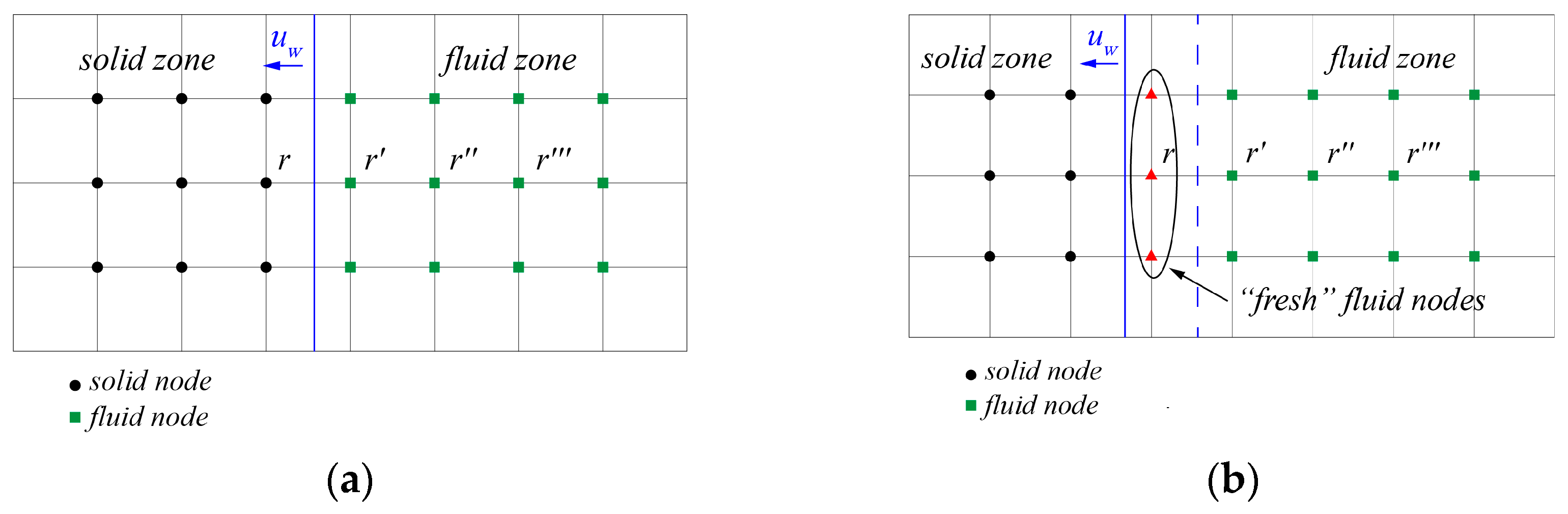
The fluid nodes and solid nodes must first be distinguished in the computational domain before processing the streaming and collision when applying the LBM to the flow issue. The type of nodes will change from solid to fluid when a moving solid wall is present in the flow field, and these “fresh” fluid nodes must be handled independently. The “fresh” fluid node is shown in Figure 1 before and after the boundary movement schematic. The blue solid line in Figure 1a is represented by the moving boundary to the left to the position of Figure 1b, and is the “fresh” fluid node for us to deal with.
In this simulation, the FEQ+FNEQ approach is used to obtain a better calculation effect. Using first-order extrapolation, this method computes the density of the “fresh” fluid node with the non-equilibrium state component. Its specific expression is as follows [17]
where is the velocity of the moving solid wall; is a “fresh” fluid node; and , , and are the three closest fluid nodes near the “fresh” node along the direction normal to the outside of the solid wall.
2.3. Force Calculation of Fluid on Solid
Ladd et al. [45] proposed a method based on momentum exchange to calculate the force on the solid by the fluid, which is mainly derived from the momentum exchange between the nodes of the fluid at the near-wall surface and the opposite direction of the solid nodes, as expressed in [46]
where is the nearest solid node near the boundary; is the nearest fluid node near the boundary; is the indicator for judging the solid zone and the fluid zone, when taking 1 for the solid zone and 0 for the fluid zone; and is the discrete velocity in the opposite direction to the discrete velocity .
2.4. Force Coefficient
Hydrodynamics’ dimensionless quantity, the force coefficient, is expressed as follows in relation to the force acting on a solid in a fluid,
where and are the force coefficients in the x and y directions, respectively. and are forces on the solid in the x and y directions, respectively. is the fluid density, is the inlet velocity, and is the area of the force.
2.5. Cavitation Number
The degree of cavitation can be expressed in terms of the cavitation number; the formula is
where is the inlet pressure; is the inlet density; and is the corresponding saturated vapor pressure.
2.6. Unit Conversion
This section will discuss the conversion method from lattice units to physical units for phase change processes in the LBM, as introduced by Wang et al. [47]. All physical quantities are constructed from base quantities, and for multiphase flow issues that involve heat transfer and mass, the standard practice is to use four fundamental units: T, , L, and M, which correspond to time t, temperature T, length l, and mass m, respectively. Grasping the conversion relationships between these fundamental physical quantities enables the derivation of transformation formulas for other physical quantities. The conversion relationships among these basic physical quantities are detailed as follows:
where PS denotes physical scale, LS signifies lattice scale, d represents conversion, and , , , and are the conversion parameters. Consequently, the unit conversion parameter for a physical quantity with dimensions can be expressed as:
where:
For the pseudo-potential model, the conversion parameters of fundamental physical quantities can be derived by combining the pseudo-potential model with the equation of state (EOS) for non-ideal conditions. For a specific fluid, important parameters such as the critical temperature , critical pressure , and gas constant can all be solved through the EOS. The physical parameter can be calculated using the parameter formula in Equation (13). However, when solving the equations, one might encounter the issue of having four unknowns but only three operational equations. This problem can be addressed by employing the method of surface tension. In the pseudo-potential model, surface tension is primarily influenced by the saturation temperature, and thus the parameter can be directly determined after the EOS parameters are established. From the above, we can derive the following conversion formulas:
For the C-S equation of state, the conversion parameters are as follows:
It can be inferred that in the pseudo-potential model, obtaining the values of parameters , , , and is possible as long as the equation of state (EOS) for a non-ideal gas and the actual fluid are known. For the liquid–vapor system utilized in this study, the corresponding parameter conversions are presented in Table 1.
2.7. Model Validation
In this study, the cascaded pseudo-potential lattice Boltzmann model and dynamic contact angle model were primarily employed to simulate the multiphase flow phenomena within the fluid and the wetting behavior at the fluid–wall interface. In order to validate the accuracy of the computational results, the Young–Laplace law was utilized to verify the setup of the pseudo-potential model. Additionally, the dynamic contact angle model was used to simulate the adhesion of liquid droplets on a flat wall under different wetting conditions, including 30°, 90° and 120°. The specific cases are illustrated in Figure 2 and Figure 3. As can be seen from Figure 2, there is a clear linear relationship between the pressure difference inside and outside the droplet and the inverse of the droplet radius , which aligns with the Young–Laplace law. This yields the surface tension of the droplet as . Figure 3 demonstrates that when flat wall surfaces with contact angles set at 30°, 90°, and 120° are considered, the droplets exhibit hydrophilic, neutral, and hydrophobic behaviors on these surfaces, respectively.
2.8. Computation Domain and Boundaries
The computational domain, as depicted in Figure 4, is a lattice region of 1000 × 800. The upper and lower right sides of the step-shaped sack wall region are set, and the entrance width is 400. The needle valves, with an initial stroke of 50, can be adjusted over time in a horizontal direction to produce a periodic reciprocating motion, and the dimensions of each part in nozzle are shown in the figure. In the calculation, the momentum exchange method was used to calculate the forces acting on the lower boundary of sack wall DE, needle valve side section AB, and top section BC, and the average value of force coefficients and for each component was used to express the forces be acted. According to findings from prior research, cavitation phenomena were observed at the lower boundary of the sack wall [42]. In light of this, our simulation designated a point F within the region of cavitation that was selected for density monitoring. Needle valve movement speed was , where the amplitude A = 200, frequency f = 1/50,000, and a complete cycle T = 50,000. This simulation set the needle valve to start moving again after the flow field was stabilized for one cycle, i.e., after 50,000 time steps.
The domain’s liquid-phase density = 0.464 and vapor-phase density = 0.000445 were set, and the ratio of liquid to vapor densities was 1042.7, which is more in line with the actual vapor–liquid condition. The upper and lower boundaries used half-way bounce-back to achieve no-slip solid wall conditions, expressed as follows [48].
where is the fluid node nearest the boundary.
The inlet is the Zou–He boundary conditions for the velocity inlet of , expressed as follows [49].
where is the pressure in the inlet boundary.
The outlet is also the Zou–He boundary conditions for the pressure outlet of , expressed as follows:
where is the velocity in the outlet boundary.
2.9. Grid-Independent Verification
Based on a needle valve frequency of f = 1/50,000, the grid-independent verification was performed for the evolution of with time of the BC section at the top of the needle valve using the three grid resolutions of 360 × 900, 400 × 1000, and 440 × 1100. As detailed in Figure 5, it is evident that the fluctuation trends under different grids are similar, with no significant discrepancies observed.
To enhance the accuracy of data validation, the 360 × 900 grid configuration was utilized as a reference standard, and the minimum two-norm method applied to verify the data errors under the other two grid resolutions. This approach is based on the computation formula for the minimum two-norm, which is defined as follows:
where is a baseline quantity.
Table 2 presents the computation results of the minimum two-norm, from which we can observe that the maximum error is only 1.84%, fully in accordance with the grid independence verification. Therefore, in this paper, the grid resolution of 400 × 1000 was chosen for the calculation.
3. Results and Discussion
The inception and evolution of cavitation in the flow field is shown in Figure 6 when the cavitation number Ca = 1.16, where the blue area represents the vapor phase region. It can be observed that the liquid flows into the nozzle from the left inlet. As it flows through the lower region of the sack wall, the flow region narrows, resulting in an increase in fluid velocity and a decrease in pressure and density. This creates conditions for the transition of the liquid phase to the vapor phase. At t = 10,000, cavitation initiates near point D in the DE section of the sack wall’s lower boundary. With the evolution of the flow, the vapor phase continuously expands downstream along the DE section, and the cavitation area in the nozzle also increases. At t = 50,000, the needle valve starts moving to the right, but it does not change the tendency of cavitation evolution at the lower boundary of the sack wall.
The change process of the streamline diagram in the flow field during one cycle of the needle valve movement is shown in Figure 7. It can be seen that the direction of the streamlines in the flow field is from left to right, and there are two vortices at the top of the needle valve. When the needle valve moves to the right, the size of the vortex gradually decreases, until the needle valve stroke is the largest, and the size of the vortex reaches the minimum. When the needle valve begins the return movement, the size of the vortex gradually increases and reaches its maximum values at the minimum stroke of the needle valve.
3.1. Evolution of Density with Time at Cavitation at f = 1/50,000
It can be seen from Figure 6 that there is cavitation generated at the lower boundary of the sack wall, so we took a point F in the cavitation area to monitor its density, and the location of point F is shown in Figure 4.
The evolution of density with time at the monitoring location for a needle valve oscillation frequency of f = 1/50,000 is shown in Figure 8. Correlated with Figure 6, cavitation starts generating between t = 9000 and 10,000, where the monitoring location density undergoes a significant decline before fluctuating with the fluid flow, with an overall decrease of about three orders of magnitude. After t = 50,000, when needle valve motion resumes, the density exhibits cyclic variation that inversely correlates with the changing overflow area, decreasing then increasing periodically.
3.2. Relationship between the Force on a Solid as a Function of Time for f = 1/50,000
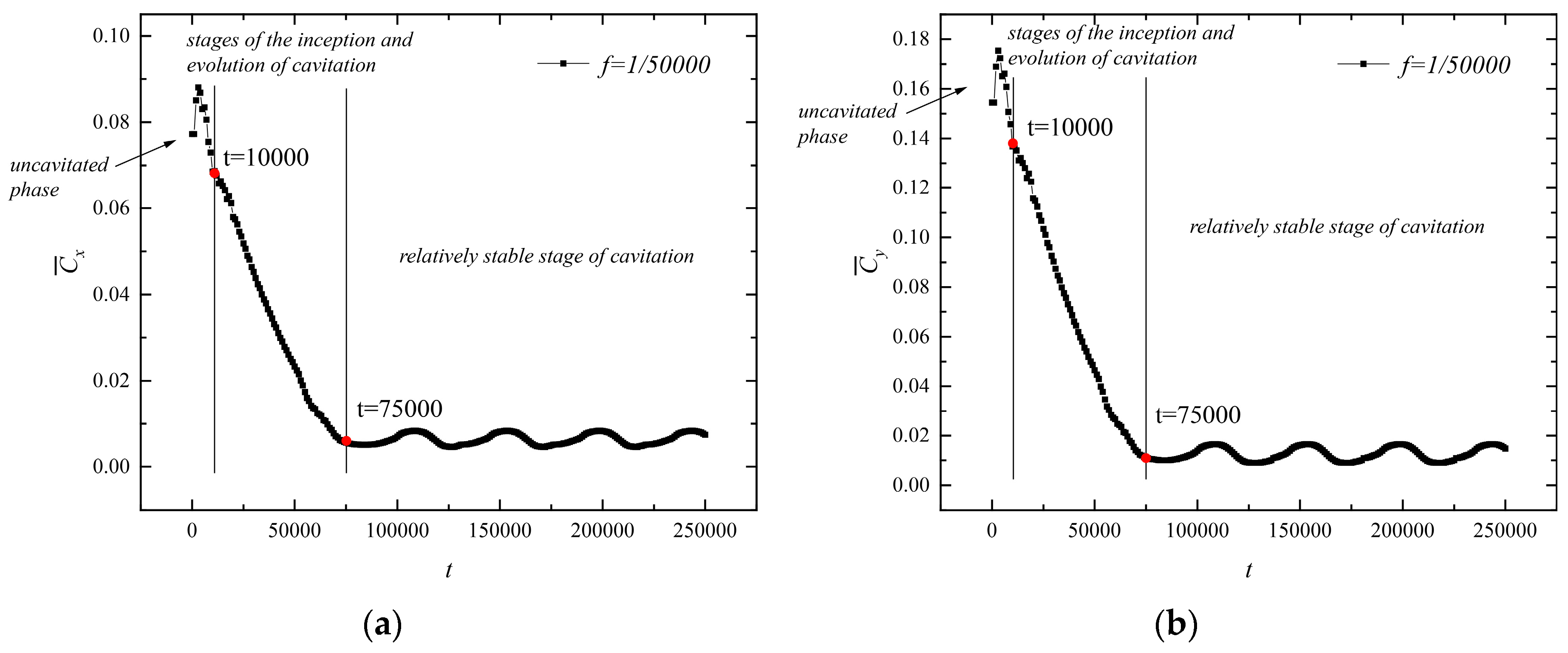
3.2.1. Forces on the Lower Boundary of the Sack Wall
The evolution of the average force coefficients of the x and y directions with time at the lower sack wall boundary DE is shown in Figure 9. Combining the two figures makes it possible to see that the cavitation begins at time t = 10,000 and ends at time t = 75,000. This means there are three stages to the force on the lower boundary of the sack wall: the unproduced cavitation stage, the inception and evolution stage, and the relative stability stage. With the occurrence of cavitation, the fluid adjacent to the DE section gradually transitions from a liquid to vapor state. This phenomenon leads to a continuous reduction in the force exerted on the lower boundary of the sack wall. When cavitation is fully developed, the force on the DE section decreases by approximately an order of magnitude compared to before cavitation initiation and exhibits periodic fluctuations within a certain range with the movement of the needle valve. Throughout the entire flow process, the DE section is always subjected to the force of the fluid acting towards its right in a horizontal direction and upward in the vertical direction.
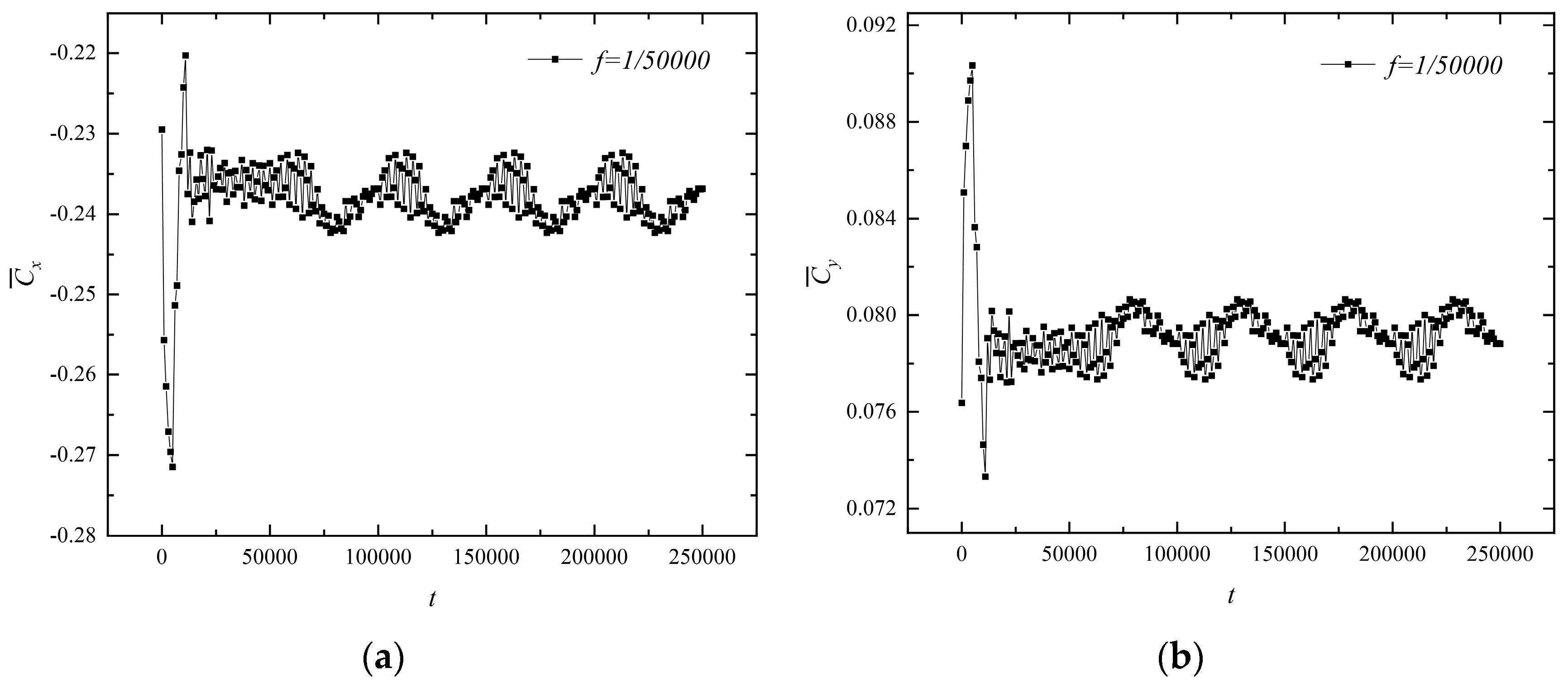
3.2.2. The Force on the Top and Side Ends of the Needle Valve
The evolution of the average force coefficients of the x and y directions with time at the top of the needle valve BC is shown in Figure 10. The two graphs demonstrate that the needle valve top is mostly subjected to leftward fluid forces in the horizontal direction and upward in the vertical direction, and the overall magnitude does not show significant changes. In the initial stage, the fluctuation of force on the BC section is primarily affected by fluid flow. As the needle valve begins to move, the force undergoes periodic fluctuations within a small range.
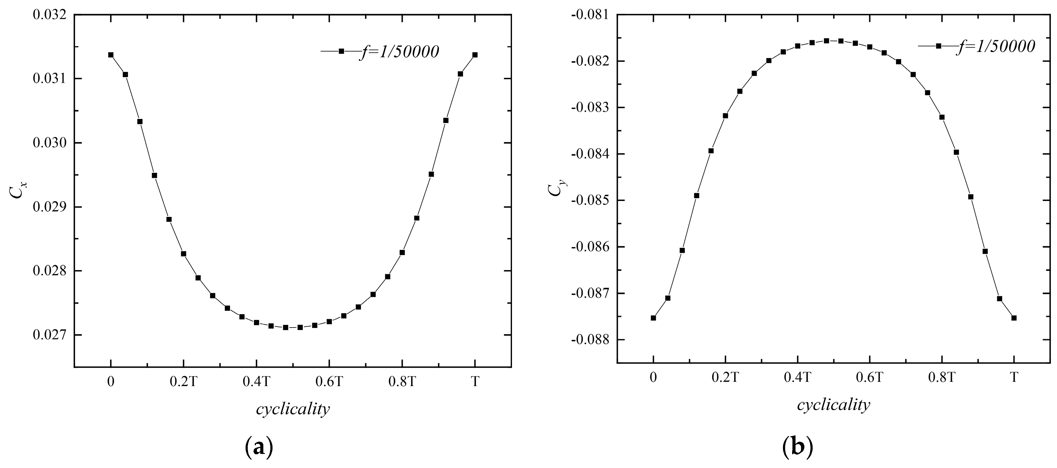
The evolution of the average force coefficients of the x and y directions at the side end of the needle valve AB is shown in Figure 11. It can be seen that the needle valve’s side end is mainly subjected to rightward fluid forces in the horizontal direction and downward in the vertical direction. As the needle valve moves to its maximum stroke position, although the length of the AB section continues to increase, the average force on this section decreases until the needle valve reaches its maximum stroke and the force reaches a minimum. In the second half of the needle valve’s motion cycle, the force on this section gradually increases and reaches its maximum at the minimum stroke of the needle valve. Moreover, in the early stage of this section, the force fluctuates with the flow of fluid, while in the later stage, it exhibits periodic variations within a small range due to the motion of the needle valve.
The diagram in Figure 7 shows two vortices at the top of the needle valve and that the vortex size gradually declines in the initial half and increases in the latter half of the cycle. Consequently, force distribution on the top of the needle valve was tallied. The force distribution on the needle valve’s side end was also counted to determine the fluid’s precise effect.
The distribution of at the top of the needle valve at a certain moment in a cycle is shown in Figure 12, from which it can be inferred that the force exhibits a symmetrical distribution phenomenon in both the x and y directions, with the axis of the computational domain being y = 400. The distribution of the force on the right boundary at the average instant of a cycle was tallied because the size of the vortex varies at different moments, which causes the force’s magnitude to vary as well.
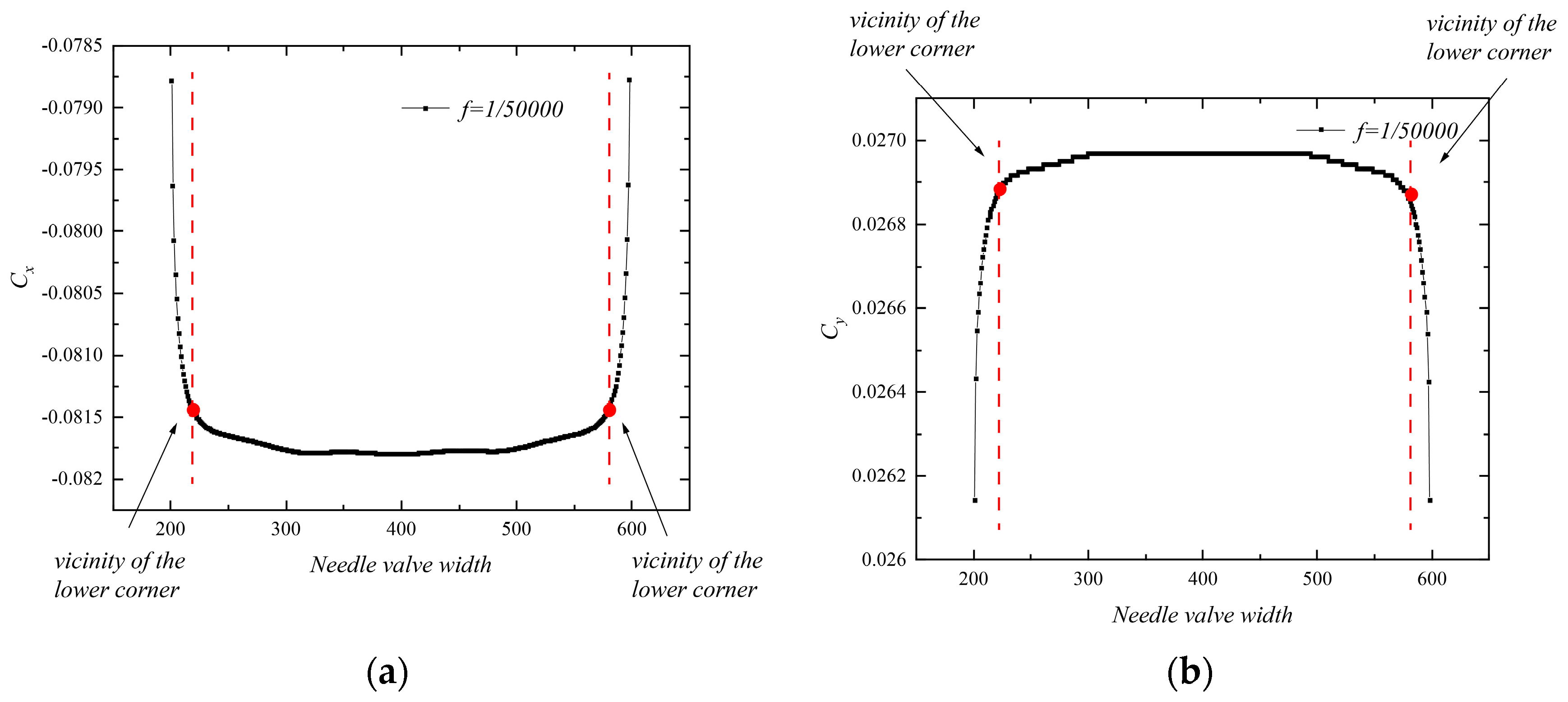
The distribution of the force coefficient of an average value over a cycle at the top of the needle valve is shown in Figure 13. It can be seen that the force at the top of the needle valve in the x and y directions shows a uniform distribution. However, the lateral fluid will affect the corner point, resulting in an inevitable drop in the distribution graph generated at the two ends.
The distribution of force coefficients along the side end of the needle valve at a particular moment is shown in Figure 14, and the evolution of force coefficients at a particular location of the side end of the needle valve during a cycle is shown in Figure 15. When the two pictures are combined, it is clear that the force in the x and y directions exhibits a decreasing distribution when the needle valve moves to the right. Additionally, throughout a single cycle, when the needle valve moves, the force magnitude at various times at the same needle valve’s upper boundary point reduces and then increases.
3.3. Effect of Needle Valve Motion Frequency on the Flow Field
Subsequently, the motion frequencies were adjusted to f = 1/40,000 and f = 1/60,000, and the results were compared with the those of the initial motion frequency of f = 1/50,000 to investigate the impact of the needle valve’s altered motion frequency on the flow field.
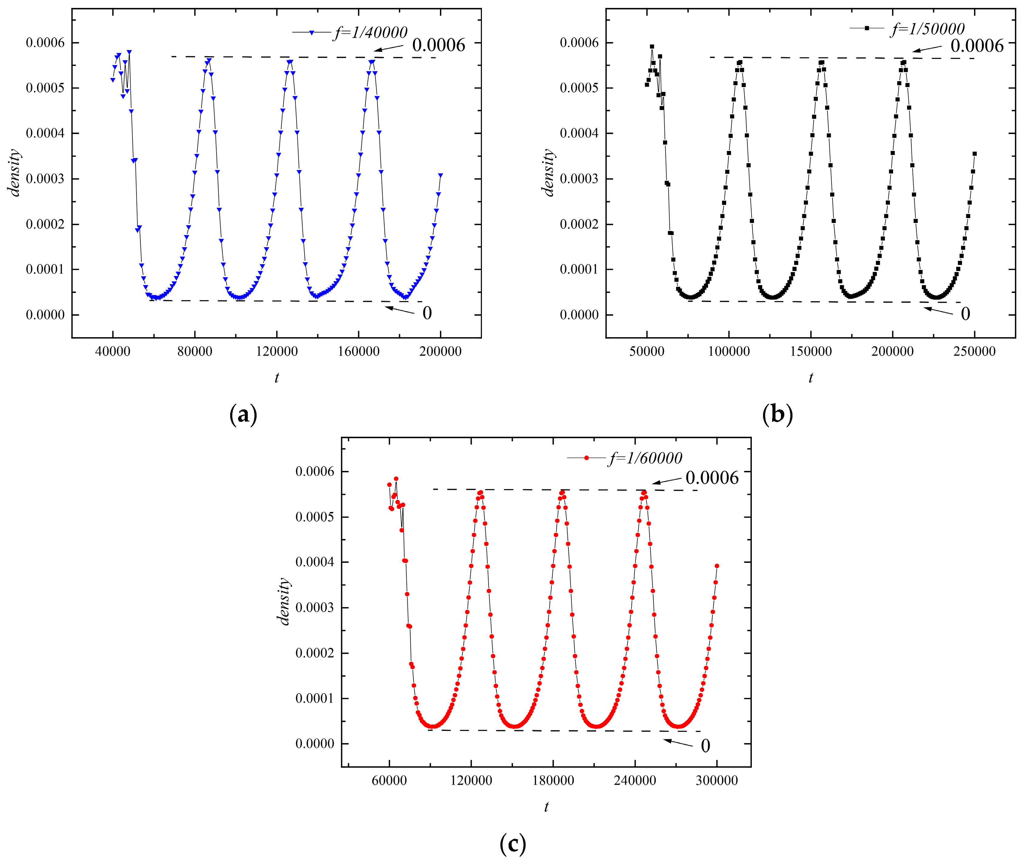
Figure 16 shows the evolution of density with time at the monitoring location under different movement frequencies of the needle valve. As can be seen from the figure, the evolution of density at the monitoring location under different frequencies shows a specific periodic change with the movement of the needle valve. However, due to the internal stability of the cavitation, the change in frequency has less of an impact on the range of density fluctuations.
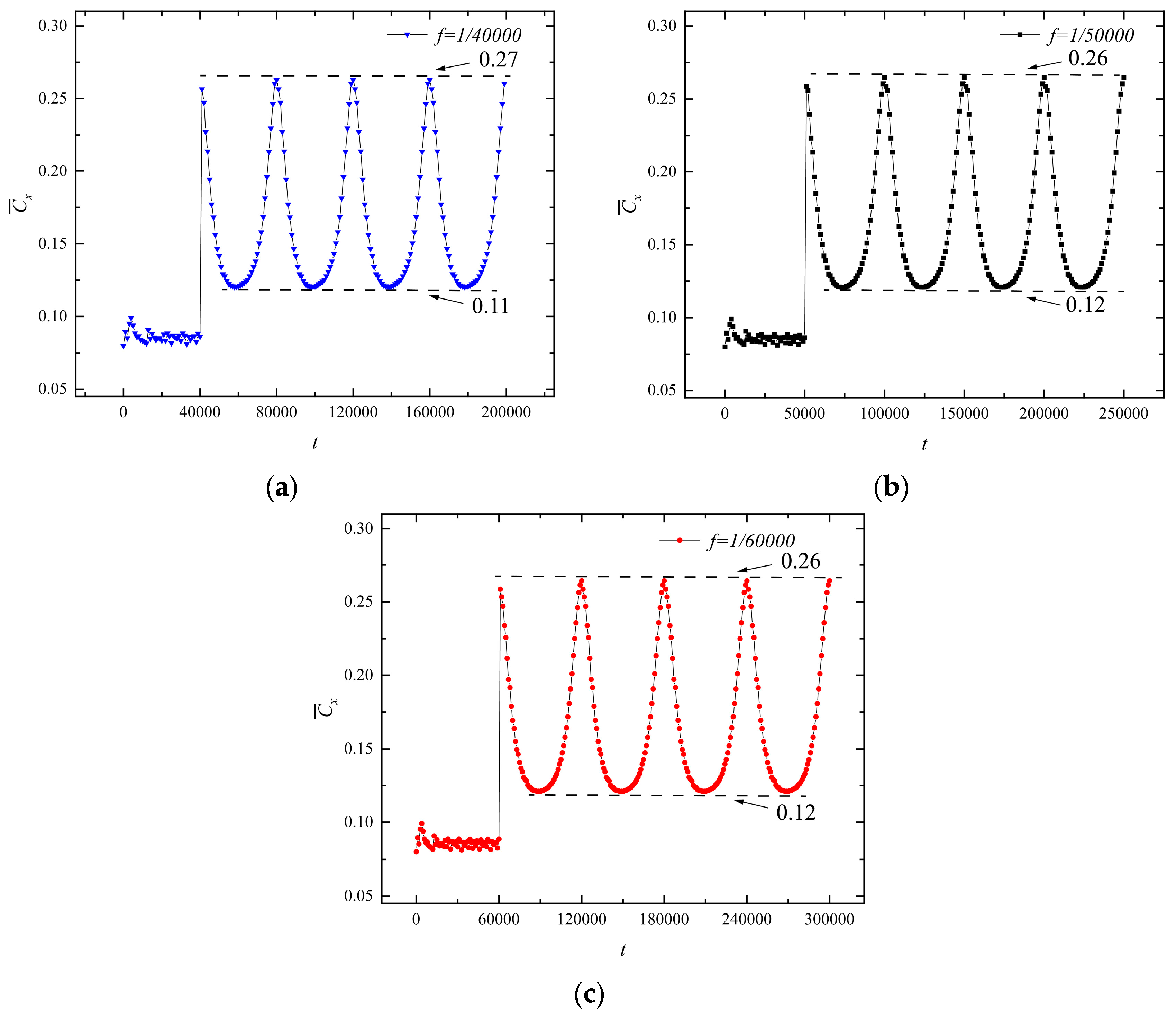
The evolutions of the average force coefficients with time at the bottom sack wall boundary DE in the x and y directions for the needle valve at various motion frequencies are displayed in Figure 17 and Figure 18, respectively. It is evident from the figures that, as the frequency increases, the cavitation generation time remains constant, but the cavitation development end time gradually delays. Overall, this does not have a significant impact on the force acting on this segment.
As previously mentioned, the side end AB section of the needle valve experiences the greatest force in the x direction as it is most affected by the valve’s motion. Consequently, this location was chosen to discuss the impact of changes in the needle valve’s motion cycle. Figure 19 illustrates the variation of force in the x direction on the AB section of the needle valve under three different motion frequencies over time. The figure shows that the fluctuation of force in the x direction at the AB section is highly synchronized with the periodic motion of the needle valve. Therefore, altering the motion cycle of the needle valve will only change the frequency of the force fluctuations in the x direction of this section without affecting the direction of the force or the amplitude of the fluctuations.
4. Conclusions and Prospects
This paper employs the cascaded pseudo-potential lattice Boltzmann model for the first time to investigate the cavitating flow field of a periodically moving needle valve in a two-dimensional nozzle in a large density case. The following conclusions are reached:
(1) The inception and evolution of cavitation at the lower boundary of the sack wall has a significant impact on the density at the cavitation region and the forces at the lower boundary of the sack wall. The density at the cavitation region decreased by approximately three orders of magnitude, while the forces on the lower boundary of the sack wall decreased by approximately one order of magnitude.
(2) The forces acting on the needle valve are mainly influenced by the cyclical motion of the needle valve. There is no cavitation phenomenon near the needle valve; therefore, the force on the needle valve does not undergo significant changes. Tangential force is the main factor in the action of the needle valve’s side end, so the fluctuation of force in the horizontal direction is more severe than that in the vertical direction.
(3) Since the vapor phase dominates the cavitation, it may be concluded from comparing the force magnitudes that the force at the sack wall’s lower boundary is less than the force at the other boundaries.
(4) In the area of cavitating flow research, acoustic effects are a significant influencing factor. However, due to the numerical simulations in this study being conducted under low-speed flow conditions and with a limited computational scope, the resulting cavitation phenomenon evolves at a slow pace. Consequently, this research has not yet delved into the analysis of acoustic aspects. Future research directions will focus on employing more refined models to tackle large-scale computation issues and integrating turbulence models to deeply investigate the characteristics of cavitation flow under high-speed conditions. Additionally, we will commit to further exploring the internal acoustic effects to gain a more comprehensive understanding.
Author Contributions
Conceptualization, F.Y.; methodology, F.Y., M.D. and H.J.; investigation, M.D. and H.J.; resources, M.D. and H.J.; data curation, M.D.; writing—original draft preparation, F.Y., M.D. and H.J.; writing—review and editing, F.Y.; supervision, F.Y. All authors have read and agreed to the published version of the manuscript.
Funding
This research received no external funding.
Data Availability Statement
Data will be made available on request.
Conflicts of Interest
The authors declare no conflicts of interest.
Nomenclature
| the current position of the particle | |
| the discrete velocity | |
| the velocity vector’s discrete direction | |
| t | the lattice time |
| the time step | |
| the distribution function of the current particle at time t | |
| the equilibrium distribution function | |
| the non-equilibrium distribution function | |
| the relaxation time | |
| the fluid viscosity | |
| the weight coefficient | |
| the lattice sound speed | |
| the lattice speed | |
| the fluid density | |
| the forcing term in space | |
| the orthogonal matrix | |
| the diagonal matrix | |
| the shift matrix | |
| the unit matrix | |
| a force vector on the moment space | |
| the velocity at the lattice point of the stream | |
| the total combined force in the system | |
| the intermolecular force | |
| the force between the fluid and the wall | |
| the gravitational force | |
| the interaction intensity parameter between particles | |
| the velocity of the moving solid wall | |
| the fresh fluid lattice node | |
| , , | the three nearest fluid lattice nodes along the direction normal to the outside of the solid wall at the fresh node |
| the nearest solid grid point near the boundary | |
| the nearest fluid grid point near the boundary | |
| the indicator for judging the solid zone and the fluid zone | |
| the discrete velocity in the opposite direction to the discrete velocity | |
| Cx | the x direction force coefficient |
| Cy | the y direction force coefficient |
| the x direction force on the solid | |
| the y direction force on the solid | |
| the area of the force | |
| the calculation domain inlet pressure | |
| the inlet density | |
| the inlet velocity | |
| the corresponding saturated vapor pressure |
References
- Zhu, Z.; Fang, S. Numerical investigation of cavitation performance of ship propellers. J. Hydrodyn. 2012, 24, 347–353. [Google Scholar] [CrossRef]
- Guo, G.; Lu, K.; Xu, S.; Yuan, J.; Bai, T.; Yang, K.; He, Z. Effects of in-nozzle liquid fuel vortex cavitation on characteristics of flow and spray, Numerical research. Int. Commun. Heat Mass Transfer. 2023, 148, 107040. [Google Scholar] [CrossRef]
- Wei, Y.; Zhang, H.; Fan, L.; Li, B.; Leng, X.; He, Z. Experimental study on influence of pressure fluctuation and cavitation characteristics of nozzle internal flow on near field spray. Fuel 2023, 337, 126843. [Google Scholar] [CrossRef]
- Yang, X.; Dong, Q.; Wang, X.; Zhou, T.; Wei, D. An experimental study on the needle valve motion characteristics of high pressure natural gas and diesel co-direct injector. Energy 2023, 265, 1126257. [Google Scholar] [CrossRef]
- Huang, W.; Moon, S.; Ohsawa, K. Near-nozzle dynamics of diesel spray under varied needle lifts and its prediction using analytical model. Fuel 2016, 180, 292–300. [Google Scholar] [CrossRef]
- Yang, F.; Yang, H.; Yan, Y.; Guo, X.; Dai, R.; Liu, C. Simulation of natural convection in an inclined polar cavity using a finite difference lattice Boltzmann method. J. Mech. Sci. Technol. 2017, 31, 3053–3065. [Google Scholar] [CrossRef]
- Silva, D.P.F.; Coelho, R.C.V.; Pagonabarraga, I.; Succi, S.; da Gama, M.M.T.; Araújo, N.A.M. Lattice Boltzmann simulation of deformable fluid-filled bodies: Progress and perspectives. Soft Matter 2024, 20, 2419–2441. [Google Scholar] [CrossRef] [PubMed]
- Wang, L.; Liu, Z.; Rajamuni, M. Recent progress of lattice Boltzmann method and its applications in fluid-structure interaction. Proc. Inst. Mech. Eng. Part C J. Mech. Eng. Sci. 2023, 237, 2461–2484. [Google Scholar] [CrossRef]
- Shirbani, M.; Siavashi, M.; Bidabadi, M. Phase Change Materials Energy Storage Enhancement Schemes and Implementing the Lattice Boltzmann Method for Simulations: A Review. Energies 2023, 16, 1059. [Google Scholar] [CrossRef]
- Yang, X.; Yang, G.; Li, S.; Shen, Q.; Miao, H.; Yuan, J. Application and development of the Lattice Boltzmann modeling in pore-scale electrodes of solid oxide fuel cells. J. Power Sources 2024, 599, 234071. [Google Scholar] [CrossRef]
- Bocanegra, J.A.; Misale, M.; Borelli, D. A systematic literature review on Lattice Boltzmann Method applied to acoustics. Eng. Anal. Bound. Elem. 2024, 158, 405–429. [Google Scholar] [CrossRef]
- Hosseini, S.A.; Boivin, P.; Thévenin, D.; Karlin, I. Lattice Boltzmann methods for combustion applications. Prog. Energy Combust. Sci. 2024, 102, 101140. [Google Scholar] [CrossRef]
- Chau Pattnaik, A.; Samanta, R.; Chattopadhyay, H. A brief on the application of multiphase lattice Boltzmann method for boiling and evaporation. J. Therm. Anal. Calorim. 2023, 148, 2869–2904. [Google Scholar] [CrossRef]
- Peskin, S.C. Flow patterns around heart valves, A numerical method. J. Comput. Phys. 1972, 10, 252–271. [Google Scholar] [CrossRef]
- Fang, H.; Wang, Z.; Lin, Z.; Liu, M. Lattice Boltzmann method for simulating the viscous flow in large distensible blood vessels. Phys. Rev. E 2002, 65, 051925. [Google Scholar] [CrossRef] [PubMed]
- Lallemand, P.; Luo, L. Lattice Boltzmann method for moving boundaries. J. Comput. Phys. 2003, 184, 406–421. [Google Scholar] [CrossRef]
- Caiazzo, A. Analysis of Lattice Boltzmann nodes initialisation in moving boundary problems. Prog. Comput. Fluid Dyn. 2008, 8, 3–10. [Google Scholar] [CrossRef]
- Krithivasan, S.; Wahal, S.; Ansumali, S. Diffused bounce-back condition and refill algorithm for the Lattice Boltzmann Method. Phys. Rev. E 2014, 89, 033313. [Google Scholar] [CrossRef] [PubMed]
- Tao, S.; Hu, J.; Guo, Z. An investigation on momentum exchange methods and refilling algorithms for lattice Boltzmann simulation of particulate flows. Comput. Fluids 2016, 133, 1–14. [Google Scholar] [CrossRef]
- Andrew, K.G.; Daniel, H.; Rothman, S.Z.; Zanetti, G. Lattice Boltzmann model of immiscible fluids. Phys. Rev. A 1991, 43, 4320–4327. [Google Scholar]
- Yang, F.; Shao, X.; Wang, Y.; Lu, Y.; Cai, X. Resistance characteristics analysis of droplet logic gate based on lattice Boltzmann method. Eur. J. Mech. B. Fluids 2021, 86, 90–106. [Google Scholar] [CrossRef]
- Shan, X.; Chen, H. Lattice Boltzmann Model for Simulating Flows with Multiple Phases and Components. Phys. Rev. E 1993, 47, 1815–1819. [Google Scholar] [CrossRef] [PubMed]
- Chen, W.; Yang, F.; Yan, Y.; Guo, X.; Dai, R.; Cai, X. Lattice Boltzmann simulation of the spreading behavior of a droplet impacting on inclined solid wall. J. Mech. Sci. Technol. 2018, 32, 2637–2649. [Google Scholar] [CrossRef]
- Swift, M.R.; Osborn, W.R.; Yeomans, J.M. Lattice Boltzmann simulation of nonideal fluids. Phys. Rev. E. 1996, 54, 5041. [Google Scholar] [CrossRef] [PubMed]
- He, X.; Chen, S.; Doolen, G.D. A novel thermal model for the Lattice Boltzmann method in incompressible limit. J. Comput. Phys. 1998, 146, 282–300. [Google Scholar] [CrossRef]
- He, X.; Chen, S.; Zhang, R. A Lattice Boltzmann scheme for incompressible multiphase flow and its application in simulation of Rayleigh-Taylor instability. J. Comput. Phys. 1999, 152, 642–663. [Google Scholar] [CrossRef]
- He, X.; Peng, H. Modeling inception and evolution of near-wall vapor thermo-cavitation bubbles via a lattice Boltzmann method. Int. J. Hydrogen Energy 2024, 49, 828–849. [Google Scholar] [CrossRef]
- He, X.; Peng, H. Contact-point analysis of attached-wall cavitation evolution on chemically patterned surfaces using the lattice Boltzmann method. Chem. Eng. Sci. 2024, 287, 119753. [Google Scholar] [CrossRef]
- He, X.; Peng, H.; Zhang, J. A lattice Boltzmann investigation of liquid viscosity effects on the evolution of a cavitation bubble attached to chemically patterned walls. Phys. Fluids 2023, 35, 093303. [Google Scholar] [CrossRef]
- Liu, Y.; Peng, Y. Study on the collapse process of cavitation bubbles including heat transfer by lattice Boltzmann method. J. Mar. Sci. Eng. 2021, 9, 219. [Google Scholar] [CrossRef]
- Li, Y.; Ouyang, J.; Peng, Y.; Liu, Y. Numerical Simulation of Cavitation Bubble Collapse inside an Inclined V-Shape Corner by Thermal Lattice Boltzmann Method. Water 2024, 16, 161. [Google Scholar] [CrossRef]
- Saritha, G.; Banerjee, R. Development and application of a high density ratio pseudopotential based two-phase LBM solver to study cavitating bubble dynamics in pressure driven channel flow at low Reynolds number. Eur. J. Mech. B Fluids 2019, 75, 83–96. [Google Scholar] [CrossRef]
- Zhu, Y.; Shan, M.; Yang, Y.; Han, Q.; Zhu, C.; Zhang, X. Effect of wettability on collapsing cavitation bubble near solid surface studied by multi-relaxation-time lattice Boltzmann model. Appl. Sci. 2018, 8, 940. [Google Scholar] [CrossRef]
- Falcucci, G.; Ubertini, S.; Bella, G.; Succi, S. Lattice Boltzmann Simulation of Cavitating Flows. Commun. Comput. Phys. 2013, 13, 685–695. [Google Scholar] [CrossRef]
- Falcucci, G.; Jannelli, E.; Ubertini, S.; Succi, S. Direct numerical evidence of stress-induced cavitation. J. Fluid Mech. 2013, 728, 362–375. [Google Scholar] [CrossRef]
- Ezzatneshan, E. Study of surface wettability effect on cavitation inception by implementation of the Lattice Boltzmann method. Phys. Fluids 2017, 29, 113304. [Google Scholar] [CrossRef]
- Sun, Z.; Cao, H.; Shan, L.; Hu, X. Lattice-Boltzmann simulation of induced cavitation in protruding structure. Numer. Heat Transf. Part A Appl. 2019, 76, 465–478. [Google Scholar] [CrossRef]
- Fei, L.; Luo, K.H. Consistent forcing scheme in the cascaded Lattice Boltzmann method. Phys. Rev. E 2017, 96, 053307. [Google Scholar] [CrossRef] [PubMed]
- Jahanshaloo, L.; Azwadi, C.; Fazeli, A.; HA, M.P. An overview of boundary implementation in Lattice Boltzmann method for computational heat and mass transfer. Int. Commun. Heat Mass Transf. 2016, 78, 1–12. [Google Scholar] [CrossRef]
- Hoseyni, A.; Dadvand, A.; Rezazadeh, S.; Mohammadi, S.K. Enhancement of mixed convection heat transfer in a square cavity via a freely moving elastic ring. Theor. Comput. Fluid Dyn. 2023, 37, 83–104. [Google Scholar] [CrossRef]
- Yuan, P.; Schaefer, L. Equations of state in a Lattice Boltzmann model. Phys. Fluids 2006, 18, 042101. [Google Scholar] [CrossRef]
- Luo, T.; Xia, J. Lattice Boltzmann simulation of low-Reynolds-number cavitating contracting-nozzle flow interacting with a moving valve. AIP Adv. 2020, 10, 125203. [Google Scholar] [CrossRef]
- Salaheddine, C.; Mohammed, J.; Ahmed, M. Numerical study of the evolution of bubbles during nucleation and droplets during condensation on a surface of variable wettability using the pseudopotential MRT-LBM method. Numer. Heat Transf. Part B 2024, 85, 131–158. [Google Scholar]
- Salaheddine, C.; Mohammed, J.; Ahmed, M. Impact process of a droplet on solid surfaces: Influence of surface wettability using lattice Boltzmann method. Eur. J. Mech. B Fluids 2024, 105, 164–179. [Google Scholar]
- Ladd, A.J.C. Numerical simulations of particulate suspensions via a discretized Boltzmann equation Part I. Theoretical Foundation. J. Fluid Mech. 1994, 271, 285–309. [Google Scholar] [CrossRef]
- Yu, D.; Mei, R.; Luo, L.; Shyy, W. Viscous flow computations with the method of lattice Boltzmann equation. Prog. Aerosp. Sci. 2003, 39, 329–367. [Google Scholar] [CrossRef]
- Wang, S.; Tong, Z.; He, Y.; Liu, X. Unit conversion in pseudopotential lattice Boltzmann method for liquid–vapor phase change simulations. Phys. Fluids 2022, 34, 103305. [Google Scholar] [CrossRef]
- Bouzidi, M.; Firdaouss, M.; Lallemand, P. Momentum transfer of a lattice Boltzmann fluid with boundaries. Phys. Fluids 2001, 13, 3452–3459. [Google Scholar] [CrossRef]
- Zou, Q.; He, X. On pressure and velocity boundary conditions for the lattice Boltzmann BGK model. Phys. Fluids 1997, 9, 1591–1598. [Google Scholar] [CrossRef]
Figure 1.
Schematic of “fresh” fluid nodes coming from the solid zone (a) before movement of solid boundary; (b) after movement of solid boundary.
Figure 1.
Schematic of “fresh” fluid nodes coming from the solid zone (a) before movement of solid boundary; (b) after movement of solid boundary.

Figure 2.
Verification of the Young–Laplace equation.

Figure 3.
Schematic diagrams of three different forms of wall wettability: (a) hydrophilic wall; (b) neutral wall; (c) hydrophobic wall.
Figure 3.
Schematic diagrams of three different forms of wall wettability: (a) hydrophilic wall; (b) neutral wall; (c) hydrophobic wall.

Figure 4.
The schematic of the computational domain.

Figure 5.
Evolution of with time of the BC section at the top of the needle valve.

Figure 6.
Inception and evolution of cavitation.

Figure 7.
Snapshots of streamline changes in the computational domain over one cycle.

Figure 8.
Evolution of density variation with time at the monitoring location.

Figure 9.
Evolution of force coefficients with time of the DE section at the lower boundary of the sack wall: (a) x direction; (b) y direction.
Figure 9.
Evolution of force coefficients with time of the DE section at the lower boundary of the sack wall: (a) x direction; (b) y direction.

Figure 10.
Evolution of force coefficients with time of the BC section at the top of the needle valve: (a) x direction; (b) y direction.
Figure 10.
Evolution of force coefficients with time of the BC section at the top of the needle valve: (a) x direction; (b) y direction.

Figure 11.
Evolution of force coefficients with time of the AB section at the side end of the needle valve: (a) x direction; (b) y direction.
Figure 11.
Evolution of force coefficients with time of the AB section at the side end of the needle valve: (a) x direction; (b) y direction.

Figure 12.
Distribution of force coefficients at the top of the needle valve at a certain moment in a cycle: (a) x direction; (b) y direction.
Figure 12.
Distribution of force coefficients at the top of the needle valve at a certain moment in a cycle: (a) x direction; (b) y direction.

Figure 13.
Distribution of force coefficients of average value over a cycle at top of needle valve: (a) x direction; (b) y direction.
Figure 13.
Distribution of force coefficients of average value over a cycle at top of needle valve: (a) x direction; (b) y direction.

Figure 14.
Distribution of force coefficients along the side end of the needle valve at a certain moment: (a) x direction; (b) y direction.
Figure 14.
Distribution of force coefficients along the side end of the needle valve at a certain moment: (a) x direction; (b) y direction.

Figure 15.
Evolution of force coefficients at a particular location of the side end of the needle valve in one cycle: (a) x direction; (b) y direction.
Figure 15.
Evolution of force coefficients at a particular location of the side end of the needle valve in one cycle: (a) x direction; (b) y direction.

Figure 16.
Evolution of density with time at monitoring location for three frequencies: (a) f = 1/40,000; (b) f = 1/50,000; (c) f = 1/60,000.
Figure 16.
Evolution of density with time at monitoring location for three frequencies: (a) f = 1/40,000; (b) f = 1/50,000; (c) f = 1/60,000.

Figure 17.
Evolution of with time of the DE section at the lower boundary of the sack wall for three frequencies: (a) f = 1/40,000; (b) f = 1/50,000; (c) f = 1/60,000.
Figure 17.
Evolution of with time of the DE section at the lower boundary of the sack wall for three frequencies: (a) f = 1/40,000; (b) f = 1/50,000; (c) f = 1/60,000.

Figure 18.
Evolution of with time of DE section at the lower boundary of the sack wall for three frequencies: (a) f = 1/40,000; (b) f = 1/50,000; (c) f = 1/60,000.
Figure 18.
Evolution of with time of DE section at the lower boundary of the sack wall for three frequencies: (a) f = 1/40,000; (b) f = 1/50,000; (c) f = 1/60,000.

Figure 19.
Evolution of with time of the AB section at the side end of the needle valve for three frequencies: (a) f = 1/40,000; (b) f = 1/50,000; (c) f = 1/60,000.
Figure 19.
Evolution of with time of the AB section at the side end of the needle valve for three frequencies: (a) f = 1/40,000; (b) f = 1/50,000; (c) f = 1/60,000.


Table 1.
Conversion of lattice scales and physical scales.
| Parameter | Lattice Unit | Physics Unit | |
|---|---|---|---|
| Surface tension and EOS parameters | 0.08 | 639.33 | |
| 1 | 0.0025 | ||
| 4 | 461.5 | ||
| 0.0412 | 0.0229 | ||
| Basic quantities conversion parameters | 2.43 × 10⁻¹³ | ||
| 2.77 × 10⁻⁴ | |||
| 3.28 × 10⁻²⁶ | |||
| 4.35 × 10⁻¹⁰ | |||
Table 2.
Results of L for different grid resolutions.
| Case Number | Grid Resolution | |
|---|---|---|
| 1 | 360 × 900 | 0 |
| 2 | 400 × 1000 | 1.84% |
| 3 | 440 × 1100 | 1.80% |
Disclaimer/Publisher’s Note: The statements, opinions and data contained in all publications are solely those of the individual author(s) and contributor(s) and not of MDPI and/or the editor(s). MDPI and/or the editor(s) disclaim responsibility for any injury to people or property resulting from any ideas, methods, instructions or products referred to in the content. |
© 2024 by the authors. Licensee MDPI, Basel, Switzerland. This article is an open access article distributed under the terms and conditions of the Creative Commons Attribution (CC BY) license (https://creativecommons.org/licenses/by/4.0/).
Share and Cite
MDPI and ACS Style
Yang, F.; Dai, M.; Jin, H. Lattice Boltzmann Simulation of Cavitating Flow in a Two-Dimensional Nozzle with Moving Needle Valve. Processes 2024, 12, 813. https://0-doi-org.brum.beds.ac.uk/10.3390/pr12040813
AMA Style
Yang F, Dai M, Jin H. Lattice Boltzmann Simulation of Cavitating Flow in a Two-Dimensional Nozzle with Moving Needle Valve. Processes. 2024; 12(4):813. https://0-doi-org.brum.beds.ac.uk/10.3390/pr12040813
Chicago/Turabian StyleYang, Fan, Mengyao Dai, and Hu Jin. 2024. "Lattice Boltzmann Simulation of Cavitating Flow in a Two-Dimensional Nozzle with Moving Needle Valve" Processes 12, no. 4: 813. https://0-doi-org.brum.beds.ac.uk/10.3390/pr12040813
Note that from the first issue of 2016, this journal uses article numbers instead of page numbers. See further details here.