
Study on the Hydrodynamic Evolution Mechanism and Drift Flow Patterns of Pipeline Gas–Liquid Flow
1
School of Economics and Management, Zhejiang University of Science and Technology, Hangzhou 310023, China
2
School of Electrical and Information Engineering, Tianjin University, Tianjin 300072, China
3
Zhejiang Qiaoshi Intelligent Industry Co., Ltd., Ningbo 315470, China
4
College of Mechanical and Automotive Engineering, Zhejiang University of Water Resources and Electric Power, Hangzhou 310018, China
*
Author to whom correspondence should be addressed.
Processes 2024, 12(4), 695; https://0-doi-org.brum.beds.ac.uk/10.3390/pr12040695
Submission received: 26 February 2024
/
Revised: 19 March 2024
/
Accepted: 25 March 2024
/
Published: 29 March 2024
(This article belongs to the Section Energy Systems)
Abstract
:The hydrodynamic characteristic of the multiphase mixed-transport pipeline is essential to guarantee safe and sustainable oil–gas transport when extracting offshore oil and gas resources. The gas–liquid two-phase transport phenomena lead to unstable flow, which significantly impacts pipeline deformation and can cause damage to the pipeline system. The formation mechanism of the mixed-transport pipeline slug flow faces significant challenges. This paper studies the formation mechanism of two-phase slug flows in mixed-transport pipelines with multiple inlet structures. A VOF-based gas–liquid slug flow mechanical model with multiple inlets is set up. With the volumetric force source term modifying strategy, the formation mechanism and flow patterns of slug flows are obtained. The research results show that the presented strategy and optimization design method can effectively simulate the formation and evolution trends of gas–liquid slug flows. Due to the convective shock process in the eight branch pipes, a bias flow phenomenon exists in the initial state and causes flow patterns to be unsteady. The gas–liquid mixture becomes relatively uniform after the flow field stabilizes. The design of the bent pipe structure results in an unbalanced flow velocity distribution and turbulence viscosity on both sides, presenting a banded distribution characteristic. The bend structure can reduce the bias phenomenon and improve sustainable transport stability. These findings provide theoretical guidance for fluid dynamics research in offshore oil and gas and chemical processes, and also offer technical support for mixed-transport pipeline sustainability transport and optimization design of channel structures.
1. Introduction
Energy is the crucial driving force for societal development and a vital foundation for sustained economic growth. In recent years, the focus of oil and gas exploration and development has shifted from terrestrial to marine extraction, moving from shallow to deep-sea regions [1,2,3]. Oil and gas are transported directly to terrestrial surface projects via combined pipelines. However, due to the complexity of the seabed terrain, the process of mixed oil and gas transmission is affected by the undulating seabed, leading to a two-phase slug flow [4,5]. The emergence of slug flow alters the flow velocity of gas and liquid phases in the pipeline, posing numerous problems and challenges for the lifespan and material costs of subsea pipelines [6]. For example, slug flow will produce shock vibration during pipeline flow, resulting in pipeline fatigue failure [7,8]. Therefore, studying the hedging flow characteristics and flow pattern evolution of gas–liquid slug flows has significant engineering application prospects [9,10,11].
The slug flow is a turbulent fluid mechanic problem significantly impacting deep-sea oil field development and production equipment design [12,13,14,15]. For example, when slug flows occur in pipe systems, pressure in the blocked pipeline rapidly increases, enhancing the backpressure at the wellhead, and in severe cases, can reduce the productivity of oil and gas wells by up to 50%. When the lengths of liquid slugs reach several riser heights, the liquid outflow at the riser outlet fluctuates significantly, leading to overflow or flow interruption in connected equipment like separators [16,17]. When severe gas–liquid alternating flow occurs in risers, operating pipelines and associated equipment experience intense vibrations, leading to damage and potentially forcing production to halt [18,19,20]. Therefore, it is essential to study the flow properties of slug flows and enhance the stability and productivity of pipeline transportation.
In response to these issues, scholars have conducted in-depth studies on slug flows, including the macroscopic laws of averaged parameters like slug length, long bubbles, and liquid holdup [21,22,23]. Due to the complexity of slug flow and limitations in experimental technology and measurement methods, there remains substantial research potential in the natural evolution of slug formation, merging, and disappearance. Pineda-Pérez et al. studied air and high-viscosity slug flows [24]. Schmelter employed three-dimensional numerical simulations of gas–liquid slug flows, considering different experiment conditions, and thereby validating the feasibility of numerical simulations [25]. Liu conducted flow pattern studies in S-shaped pipelines, categorizing flow patterns observed in pressure and differential pressure fluctuations into five types, achieving an accurate identification rate of 90.44% [26]. Li constructed an S-shaped riser system. They identified severe transitional slug flow and stable flow by adjusting the inlet flow, analyzing significant differences in the liquid holdup and corresponding probability density distributions for each flow type [27].
From a review of the literature above, it is evident that current research on gas–liquid slug flows primarily focuses on aspects such as pressure fluctuations, slug frequency, and liquid holdup. While many studies are experimentally based, there is a discrepancy between research outcomes and actual field data due to experimental sites and equipment limitations. Hence, there is a need to undertake theoretical research and numerical simulation studies. Moreover, research on gas–liquid slug flows located at complex pipelines with multiple inlets is relatively scarce, and further exploration is needed in multiphase flow modeling and solution methods.
In general, we present a modeling and solving technology for the gas–liquid slug flows in multi-inlet systems to explore turbulent flow patterns integrated with the turbulence model. It explores flow patterns of gas–liquid slug flows within complex channels. Relevant findings can offer theoretical guidance for analyzing the feature patterns of severe slug flows in pipeline transportation systems in the marine and chemical engineering fields. Additionally, these results provide technical support for the optimization design of marine oil and gas transportation pipelines and slug flow suppression.
2. Slug Flow Mathematical Model
2.1. Gas–Liquid Flow Field Model
At present, the formation conditions and mechanism of severe slug flow are still debated, but for the riser system composed of inclined pipes and risers, the majority of the literature holds the same view: For an inclined pipe, a liquid plug can be formed in the riser to prevent the gas phase from entering the riser. In the inclined pipe, gas continues to flow into the riser system, and the squeezed liquid gradually enters the riser system. At the same time, the rising liquid pressure in the riser blocks gas from entering the pipeline, and finally, the phenomenon of the liquid plug increasing to reach the height of the riser occurs. The formation principle can be summarized as follows: when the gas and liquid at the inlet of the dip pipe flow in layers, the liquid will accumulate at the elbow under the action of gravity to form a liquid plug [28,29,30]. The liquid plug will compress the gas in the downdip pipe, resulting in an increase in the air pressure in the downdip pipe and in the height of the liquid plug in the riser pipe. The increased liquid plug in the riser further compresses the gas, which further increases the pressure in the downdip tube. When the height of the liquid plug is greater than the height of the riser, a serious slug flow phenomenon will occur.
Numerical methods can be implemented to study slug flow in pipelines. The VOF model is an interface track approach that captures and tracks interfaces [31,32]. Here, the q-phase volume fraction is αq; then, three situations can arise: If αq = 0, it indicates that the q-phase fluid is absent; if αq = 1, the liquid fills; if 0 < αq < 1, cells include interfaces and one or more phases. The continuity equations can achieve the interface track. The q-phase equations can be obtained:
where ρq is the q phase density, vq is the q phase velocity, and Sαq is the source term. The properties in the equation can be determined in a cell. The density can be obtained:
For n-phase systems, the average density can be expressed:
The fluid properties, such as viscosity, can be calculated. The momentum equation is obtained:
The energy equation is owned:
Properties and effective heat conduction are shared among the phases. The source terms include attributes related to radiation and other heat sources.
2.2. Volumetric Force Source Term Model
Gravity and the surface tension of gas–liquid phases affect the gas–liquid slug flows. The momentum equation can be obtained from surface tension source terms and gravity source terms, where the gravity source term is a volumetric force [33,34,35]. Surface tension arises from the difference in intermolecular forces at the gas–liquid boundary, requiring conversion into a volumetric force to introduce the momentum equation [36,37,38].
where g represents the vector of gravitational acceleration.
In the calculation, the surface tensions can be viewed as a constant, and curvature radius and tension coefficient should be considered as follows:
2.3. Standard k-ε Turbulence Model
For turbulent flow inside pipes, whether in a steady-state or an unsteady-state two-phase coupling scenario, the standard k-ε turbulence model is highly applicable [41,42,43,44]. Standard forms of k and ε equations are obtained:
where Gk denotes the turbulent energy term since the change in mean speed gradients; σk and σε denote the Prandtl amount of turbulent energy and the dissipation rate, respectively; YM is the total dissipation rate with respect to the pulsatile expansion; Gb is the turbulent energy term due to buoyancy; and the values of empirical parameters are as follows: C1 = 1.44, C2 = 1.92, C3 = 0.09. The turbulent viscosity coefficient μt is as follows:
3. Simulation Model of Gas–Liquid Slug Flows
3.1. Physical and Numerical Models
The construction of the slug flow model is divided into two parts: a geometric model and a finite element model. According to the established mathematical slug flow model, the system of partial differential equations is not easy to solve directly [48,49,50]. This chapter relies on the Fluent 15.0 software platform to solve the partial differential equations in order to obtain the approximate solution and meet the analysis needs. For the complex slug flow model, it is essential to establish a reasonable calculation area and carry out numerical discretions to obtain accurate numerical results.
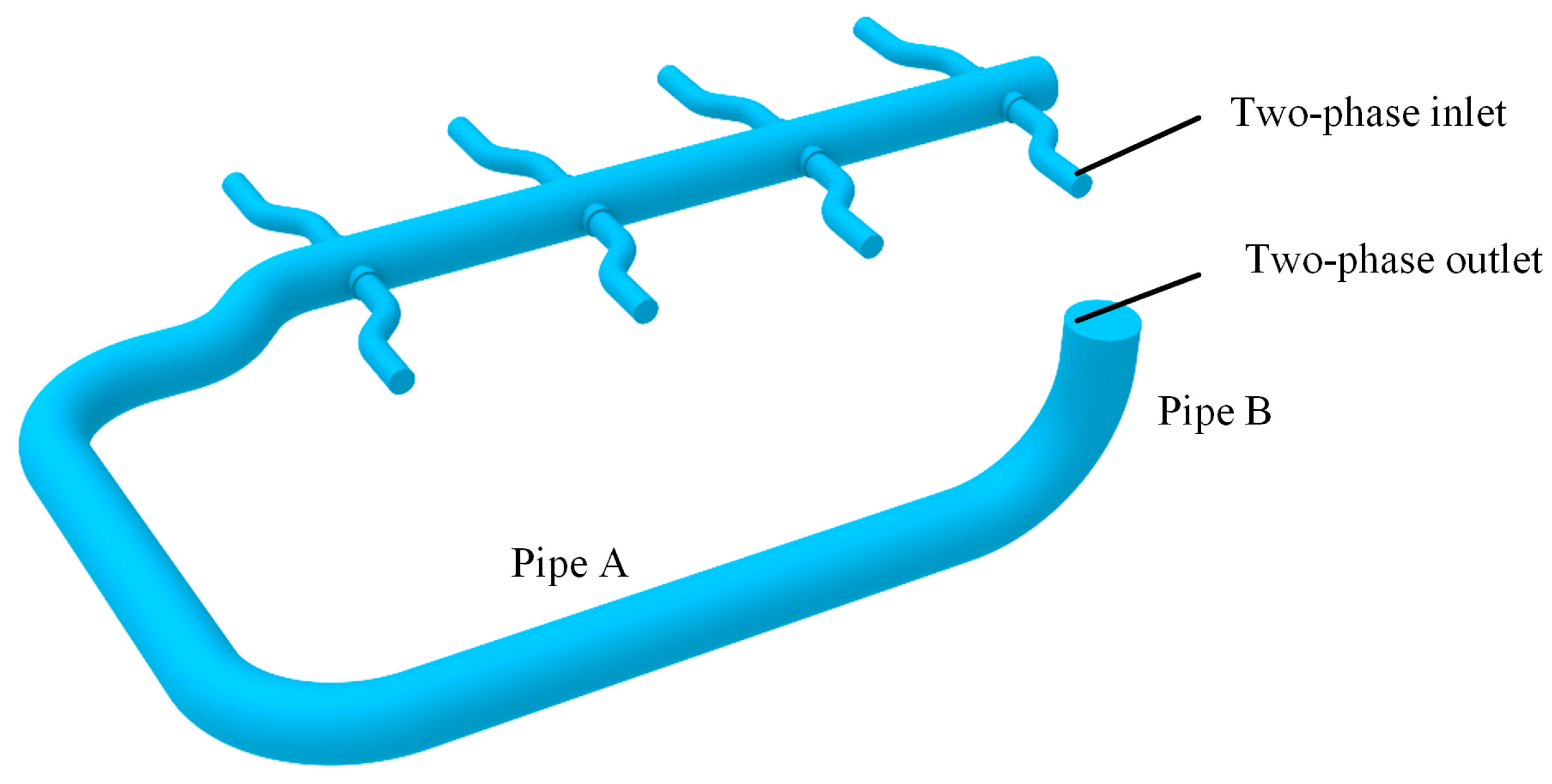
To analyze the dynamic feature of slug flows, a pipeline geometry model is obtained, as illustrated in Figure 1. Typically, the choice of the model closely aligns with the pipeline’s actual conditions. However, it requires significantly more effort, such as in grid division and time for iterative convergence, compared to two-dimensional models. The three-dimensional geometric model in this study is not symmetrically distributed, thus necessitating the development of a three-dimensional pipeline slug flow geometric model. This model comprises eight symmetrically distributed inlets, with the center coordinates of each branch indicated in the figure. The inlet diameter is 220 mm, and outlet is 508 mm. Gas–liquid fluids enter the inlets into branch pipes, converge into the main pipe, and exit through the outlet.
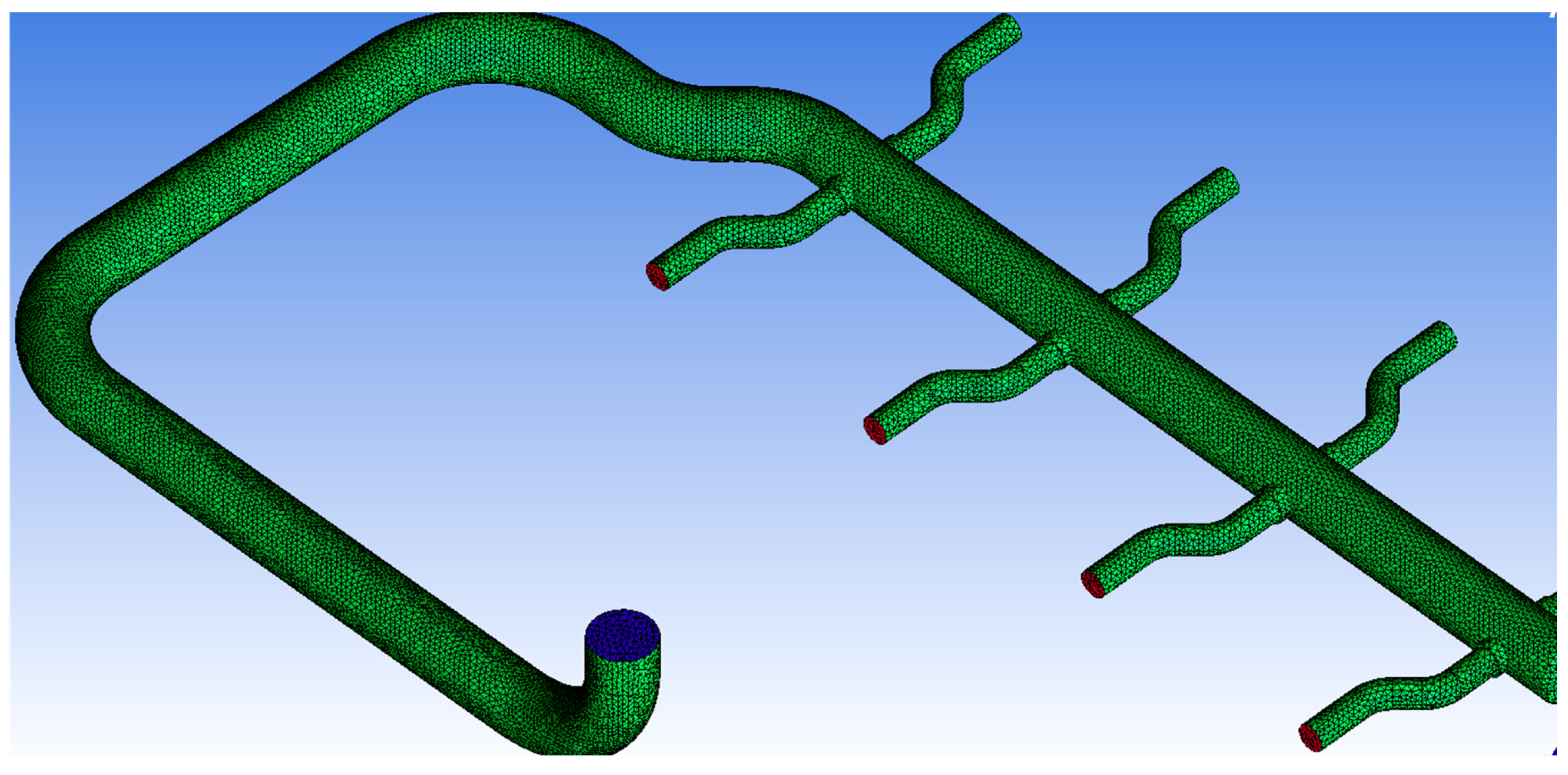
According to the multi-inlet pipeline geometric model, a pipe numerical model is set up, as shown in Figure 2. Here, the unstructured grids are used to generate numerical models. Considering the significant viscous effects and large flow field gradient changes near the pipeline walls, it is necessary to refine the grid at the walls and the inlets and outlets. An unstructured grid with a grid size of 0.002 mm, totaling 347,820 grids, and a grid quality above 0.6 is used for the pipeline inlets. For other three-dimensional numerical model fluid domains, an unstructured grid with a scale of 0.03 mm is used, totaling 458,760 grids with a grid quality above 0.5. The total number of grids for the fluid domain is 806,580, ensuring that the grid quality within the computational limits meets the accuracy requirements.
3.2. Boundary Conditions and Solution Conditions
In the model, the inlet boundary is the mass flow condition, and the flux is 45,031 kg/h. Here, the gas volume fraction is set as 30%. The gas–liquid slug flow simulation uses the transient VOF model, with explicit time discretization selected. The eight pipeline inlets are set as mass flow inlets, the container walls are no-slip walls, and the outlet is a mass flow outlet. Pressure is discretized using the PRESTO method to prevent significant pressure fluctuations. The pressure implicit with the PISO algorithm guarantees numerical convergence efficiency [51,52,53,54].
3.3. Grid Independence Validation
Grid quantity impacts computational efficiency and results [55,56,57,58,59,60]. An excessive number of grids in the computational domain prolongs the computation time and reduces the efficiency, whereas too few grids result in low accuracy of the simulation results. Hence, an appropriate number of grids should be chosen for simulation. In this study, pressure is a critical characteristic parameter, so the pressure data of the pipeline are selected for grid model independence verification. The chosen medias are gas and oil, with oil considered an incompressible phase, neglecting the impact of temperature. The grid independence verification is shown in Table 1.
In Table 1, the minimum relative error in the pressure data calculated by grid models 2 and 3 is minimal, with the minimum relative error not exceeding 1.1%. As the model grid is lesser, the numerical relative error is larger. Therefore, when the error from two grid calculations is minimal, choosing a grid model with fewer grids can satisfy accuracy requirements while improving computational efficiency. Hence, this study adopts the number of grids in grid model 2.
4. Numerical Results and Analysis
4.1. Gas-Phase Slug Flow Evolution Course
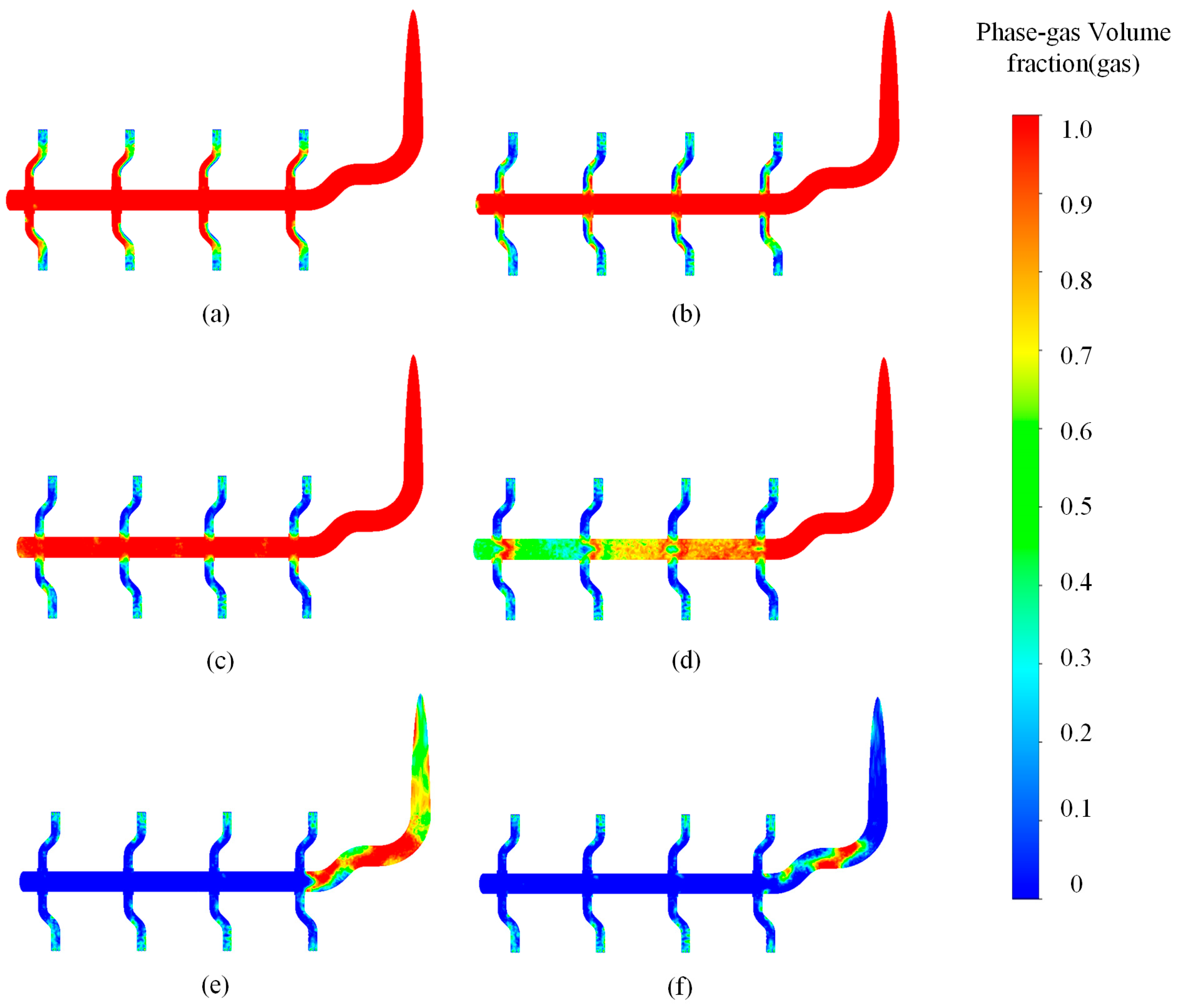
In order to study the hydrodynamic characteristics, we selected a cross-section of the pipeline model with an inlet to analyze the flow properties. The gas-phase volume fraction over time was obtained to investigate the evolution courses of gas–liquid mixed flows (Figure 3). The red areas represent the gas phase, and the blue areas denote the oil phase. The cloud diagram effect which formed was similar to the actual gas–liquid distribution. Thus, the volume fraction diagram can serve as a standard for judging the flow pattern inside the pipe.
In Figure 3, the distribution of the gas-phase volume fraction is uneven. Due to the effect of inflation, the gas phase volume fraction at the entrance is higher. In Figure 3a, the gas phase is larger on the left side of the upper part of the pipeline, and there is a bias flow phenomenon due to the structural design of the inlet pipe throughout the flow field’s evolution. When the fluids from the eight branch pipelines converge in the main pipeline, there is significant counterflow disturbance in the convergence process, making the gas-phase distribution more complex. Generally, the gas phase volume fraction is larger on the left side of the pipe. In Figure 3b–d, it is shown that the mixing process between the gas and liquid phases became more complex as the fluid field evolved, causing the best gas–liquid mixed effects. In Figure 3d,e, the branch pipe is filled with oil phase with scattered gas phase, and there is obvious slug flow in the main pipe. The above phenomena illustrate that when the flow field evolves, the gas–liquid mixing is no longer affected by the inlet pipe, and the gas phase distribution of the mixed flow field becomes complex and forms slug flows.
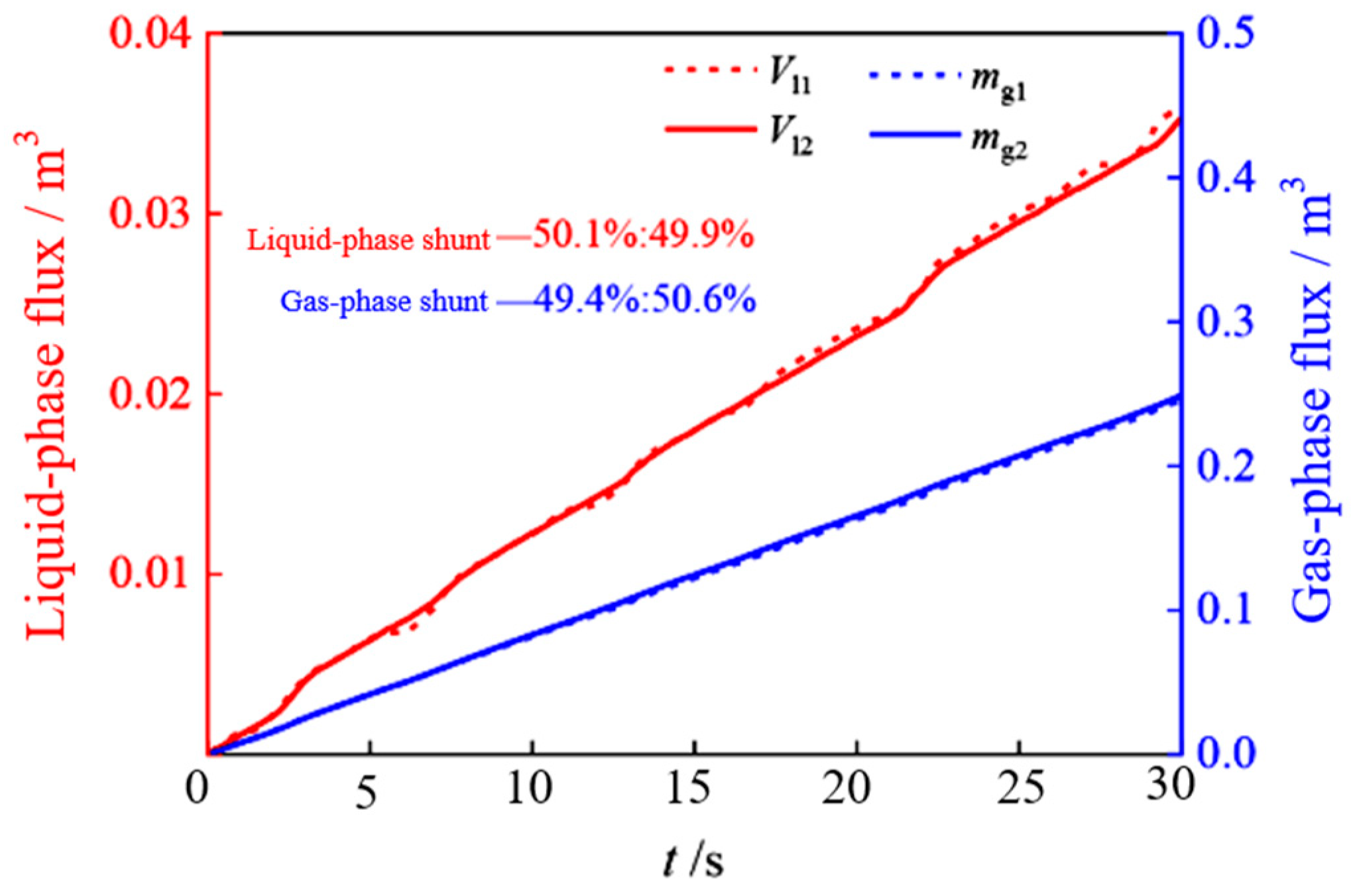
To investigate gas–liquid slug flows, mass change curves on both sides of the leftmost branch pipe were obtained at the stability state, as shown in Figure 4. No obvious bias occurred in either gas–liquid phase. Due to the intermittent character of the liquid plug, the cumulative flow curve of the liquid phase in Figure 4 fluctuated and rose. The two flow curves roughly coincided; that is, the liquid distribution was equal to the flow distribution, which verifies that the time of the liquid plug in the two branch pipelines to the intersection pipeline was consistent. The cumulative flow curve of the gas phase flow was two straight lines with a constant slope, mainly related to gas compressibility. Two flow curves of the gas phase roughly coincided, indicating that the gas phase achieved equal flow distribution. It can be seen from the measurement results that there was no apparent bias between the gas and liquid phases in the upper or lower branch pipelines. That is, the slug flow is not biased under symmetrical pipelines.
The gas–liquid flow properties after the intersection at the first interchange were obtained to discuss the two-phase flux properties. The flow of the liquid plug on both sides of the rightmost pipeline was not synchronized, and the results are shown in Figure 5. As shown in Figure 5, the fluctuation mode of the two curves of the liquid cumulative flow rate was alternately rising, indicating that there was a certain deviation before and after the time when the liquid plug in the two branch pipelines reached the intersection pipeline, mainly because the pipe conditions of the two branch pipelines were not completely symmetrical due to the different connected bend structures. From a short-term point of view, the liquid phase appeared to have a particular bias, but this bias was only temporary. The flow measurement results showed no apparent bias in the liquid phase during a long period of time. For the gas-phase flux curves, it can be found that the gas-phase had no apparent bias and took on steady evolution trends. The above phenomena illustrate that, in the process of the intersection of two gas–liquid phases in the pipeline, the flow rate of the liquid phase changes to a certain extent under the disturbance of the gas phase impact, but the gas phase content is fixed, so there is no obvious bias flow.
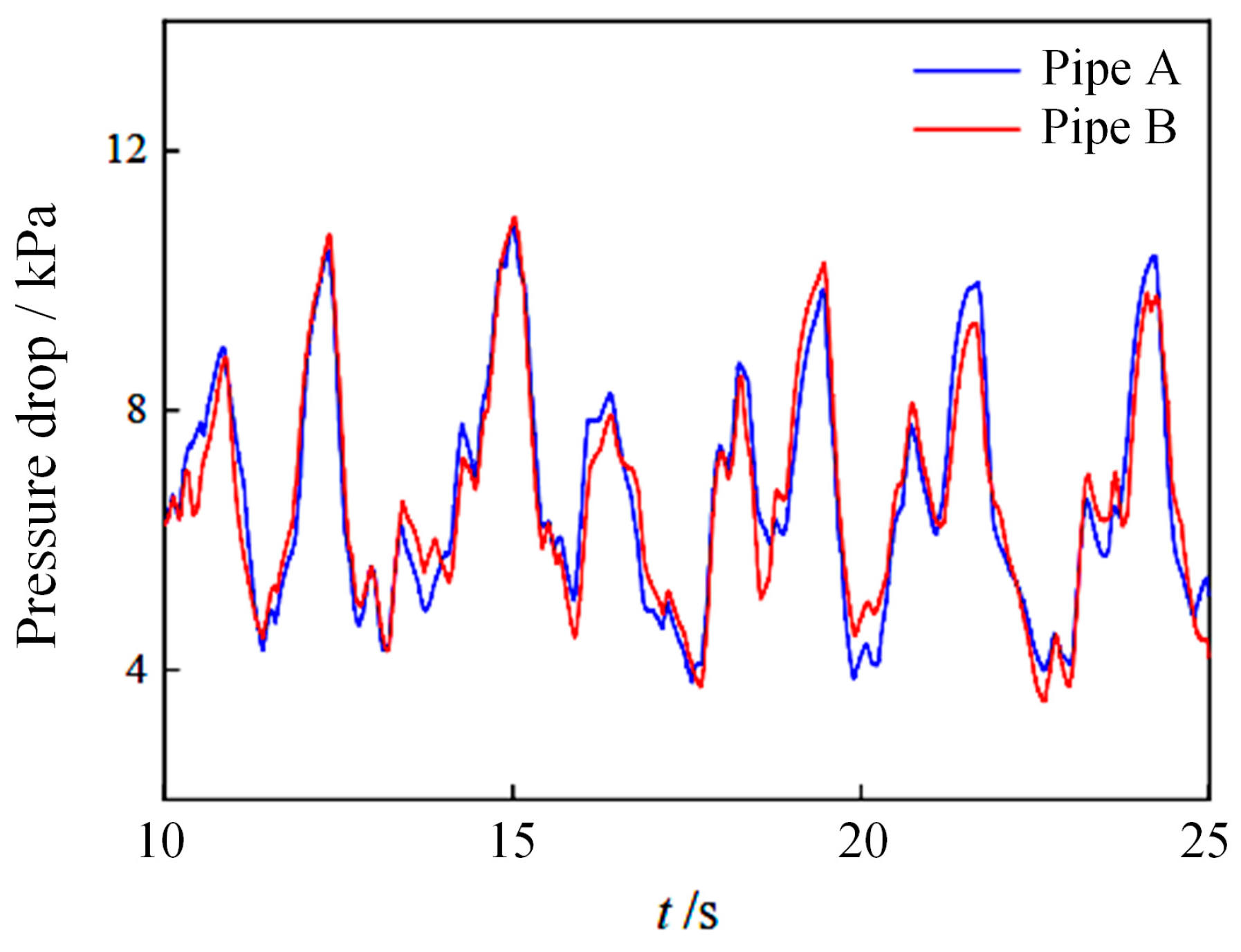
To study the pipe pressure loss, the pressure drop evolution over time was obtained, as shown in Figure 6. The branch pipe of pipeline structure A was a horizontal pipe its pressure drop was mainly a frictional loss, and the measured pressure drop loss did not exceed 2 kPa. The branch pipe of pipeline structure B contained a riser section, and its pressure drop included gravity loss and friction loss. Figure 6 shows the pressure drop curves. As can be seen from the figure, the pressure fluctuation in the pipeline presented a drastic change characteristic, and there was no obvious rule. This phenomenon is related to the scale and scale of slug formation. When the slug is formed, there is a complex flow pattern in the gas–liquid mixing process, resulting in complex changes in the shape of the slug, which made the pressure values at different positions different. In addition, it can be seen from the pressure drop of the two pipelines that the pressure drop fluctuation presented a similarly changing trend.
In the numerical model, a cross-section at the junction of the branch pipes was selected as the monitoring surface, as shown in Figure 7. The bias flow features of the mixing processes were analyzed by comparing the data from the monitoring cross-section. During this process, the fluid convergence in the branch pipes on both sides of the main pipeline created a counterflow phenomenon, potentially causing complex gas–liquid coupled disturbances, leading to uneven gas-phase distribution on both sides.
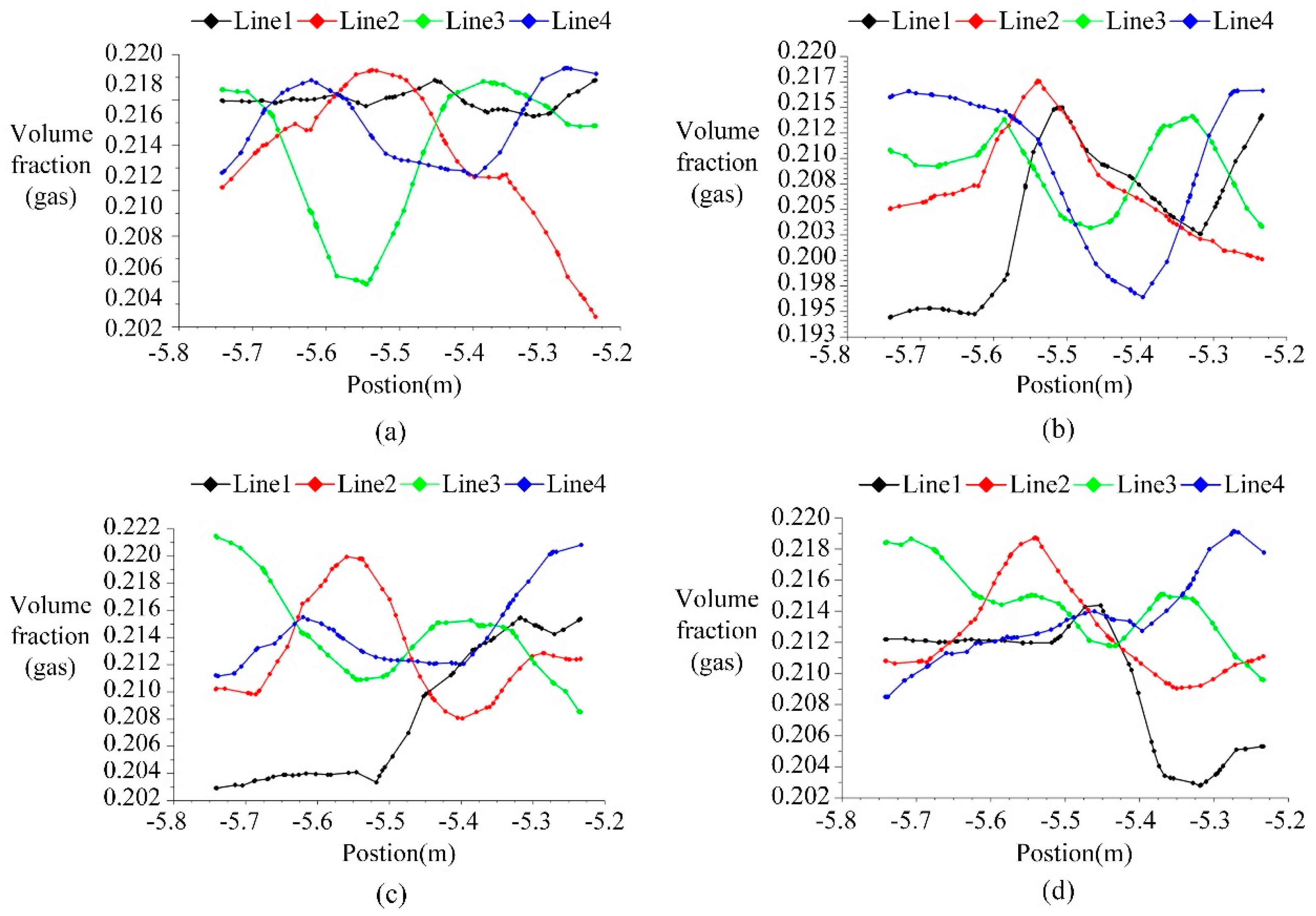
Figure 8 depicts the curves of gas-phase volume fractions at different locations. In Figure 8a, the minimum value of volume fraction is 0.1, and the maximum is 0.22. At line 1, the deviation in volume fraction is slight, indicating a relatively uniform gas phase distribution. At line 2, the volume fraction distribution is uneven between the upper and lower sides of the pipeline, with a volume fraction difference of 0.12, indicating gas–liquid solid two-phase coupling at this location. In line 3, the volume fraction is the smallest at the pipe center, with a more uniform distribution on both sides. As the fluid field dynamically evolves (Figure 8b–d), there is a noticeable gradient difference at line 1 due to the counterflow process of the gas–liquid mixing. The volume fraction distribution at other lines does not differ significantly, presenting a uniform evolutionary state.
4.2. Flow Field Velocity Evolution Characteristics
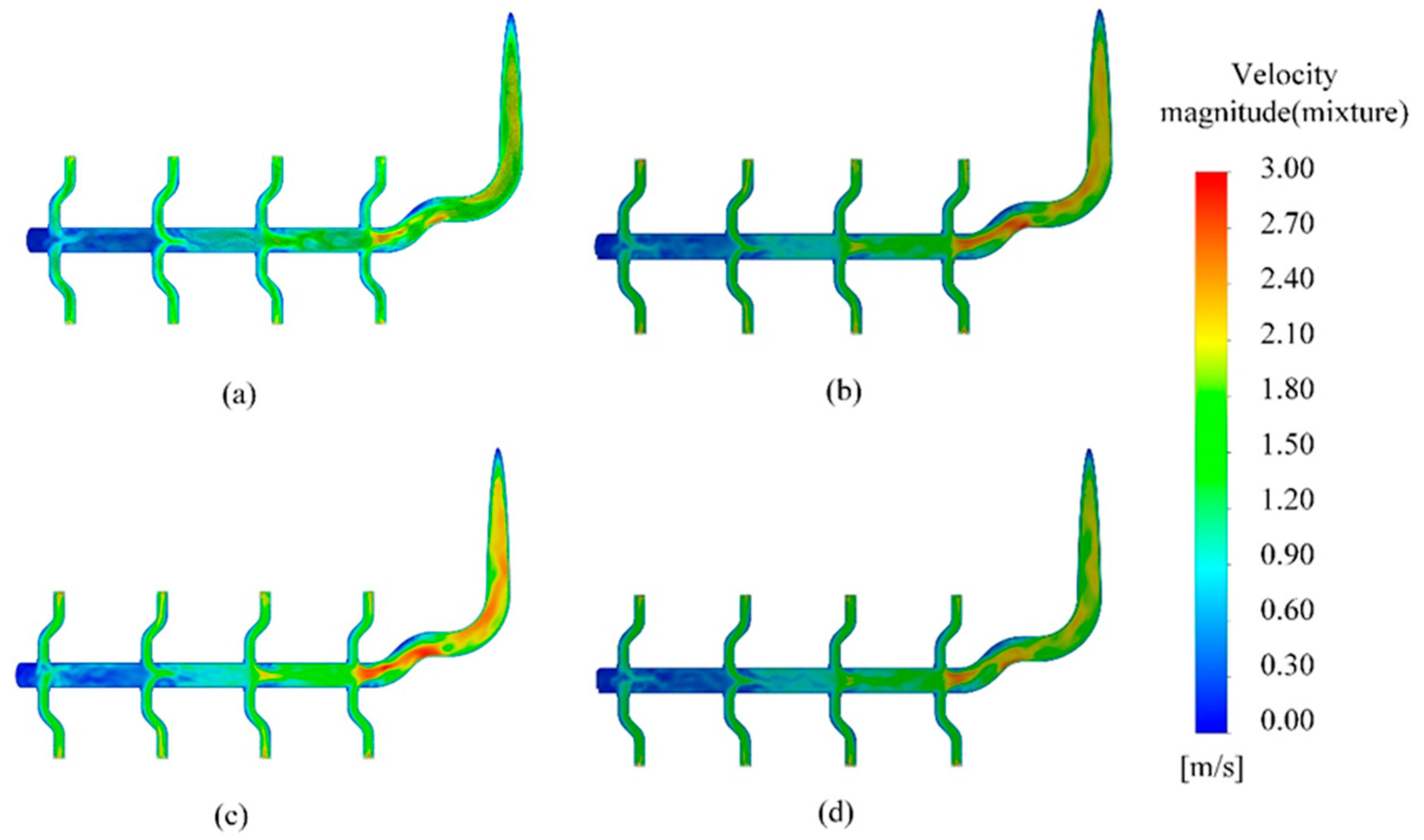
The velocity features can explain the change course of gas-phase volume fraction. Figure 9 shows the velocity contour maps at variable time sequences. In Figure 9a, at the junction of the first and second branch pipes, a specific velocity deviation exists, leading to an uneven distribution of components on both sides of the pipeline. At the junction of the third and fourth branch pipes, velocity distribution is uniform with a low-velocity area. However, at the end of the fourth branch pipe, the flow field’s velocity reaches a local maximum of 3 m/s, and the fluid velocity at the bend is uneven, with a noticeable bias flow phenomenon.
As the gas–liquid flow evolves, the bias flow at the bend sides becomes more severe, and the min and max velocities are 0.27 m/s and 2.7 m/s (Figure 9b). In Figure 9c, the flow velocity at the first branch has a significant disturbance, resulting in a large velocity gradient. However, the pipeline flow becomes uniform after converging at the third branch. At this point, the maximum velocity occurs at the fourth branch, where the bend’s structure causes a large difference in fluid velocity. In Figure 9d, the entire velocity reaches a stable state, with the bias flow at the bend reduced, showing a phenomenon wherein the flow speed takes on faster speeds at the lower sides and slower at the upper sides. Therefore, in order to avoid the occurrence of this phenomenon, it is of great significance to optimize the design of the bending pipe structure.
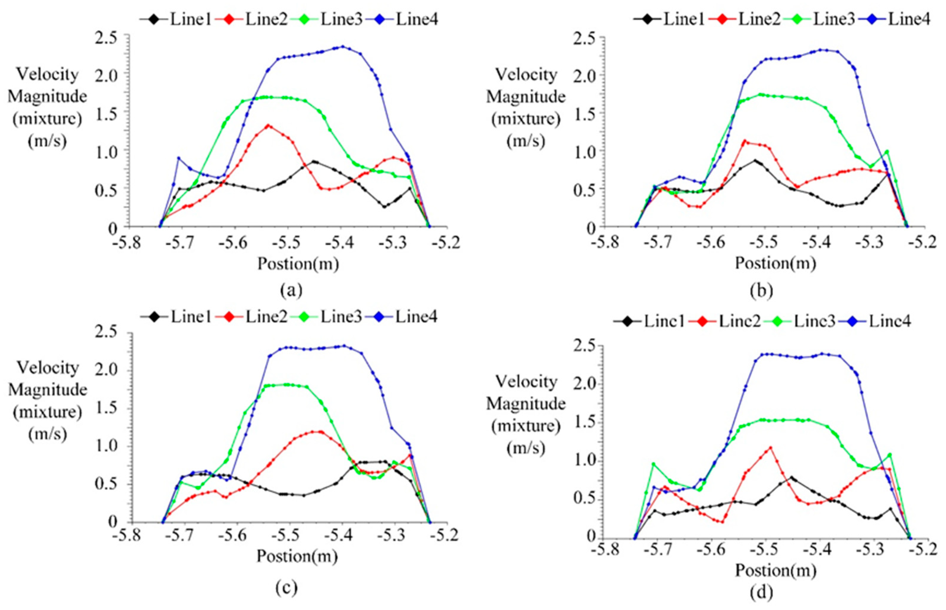
Fluid velocity curves at different locations were obtained (Figure 10). The fluid speed near the pipeline walls was lower, mainly due to the walls’ viscous resistances. At the center of the pipeline, the fluid velocity was greater, reaching its maximum at the junction of the fourth branch pipe. Overall, there was no difference in the fluid velocity at the lower and upper sides near the pipeline walls after stabilization. This suggests a relatively uniform mixing of the gas and liquid phases. The above phenomenon shows that there was no obvious bias in the stabilized flow field. The high velocity of the fourth pipe interchange is related to the design of the connected pipe’s bend structure.
4.3. Evolution Characteristics of Flow Field Turbulent Viscosity
The turbulent viscosity is a vital parameter to describe the flow properties. To explore evolution trends of slug flows, the turbulent viscosity changes are obtained, as shown in Figure 11. In Figure 11a, localized nesting of turbulent vortices occurs at the junction of the first branch pipe, resulting in greater turbulent viscosity. At the junction of the second branch pipe, the turbulent viscosity on upper sides is more significant than that on lower sides. At the junction of third branch pipe, the turbulent viscosity remains uniform on the pipeline and shows a banded distribution near the wall. At the junction of the fourth branch pipe, the lower side of the bend has greater turbulent viscosity, uniformly distributed along the pipe wall, indicating higher turbulent energy at the bend. In Figure 11b, the maximum turbulent viscosity in the entire flow field is reduced compared to the maximum value in Figure 11a. However, the distribution of turbulent viscosity becomes more random and disordered. In Figure 11c,d, the turbulent viscosity inside the pipeline is influenced by the viscous resistance of the walls and is distributed along the pipeline wall. The turbulent viscosity distribution at each branch pipe junction is uniform, and the entire flow field reaches a stable mixed flow state.
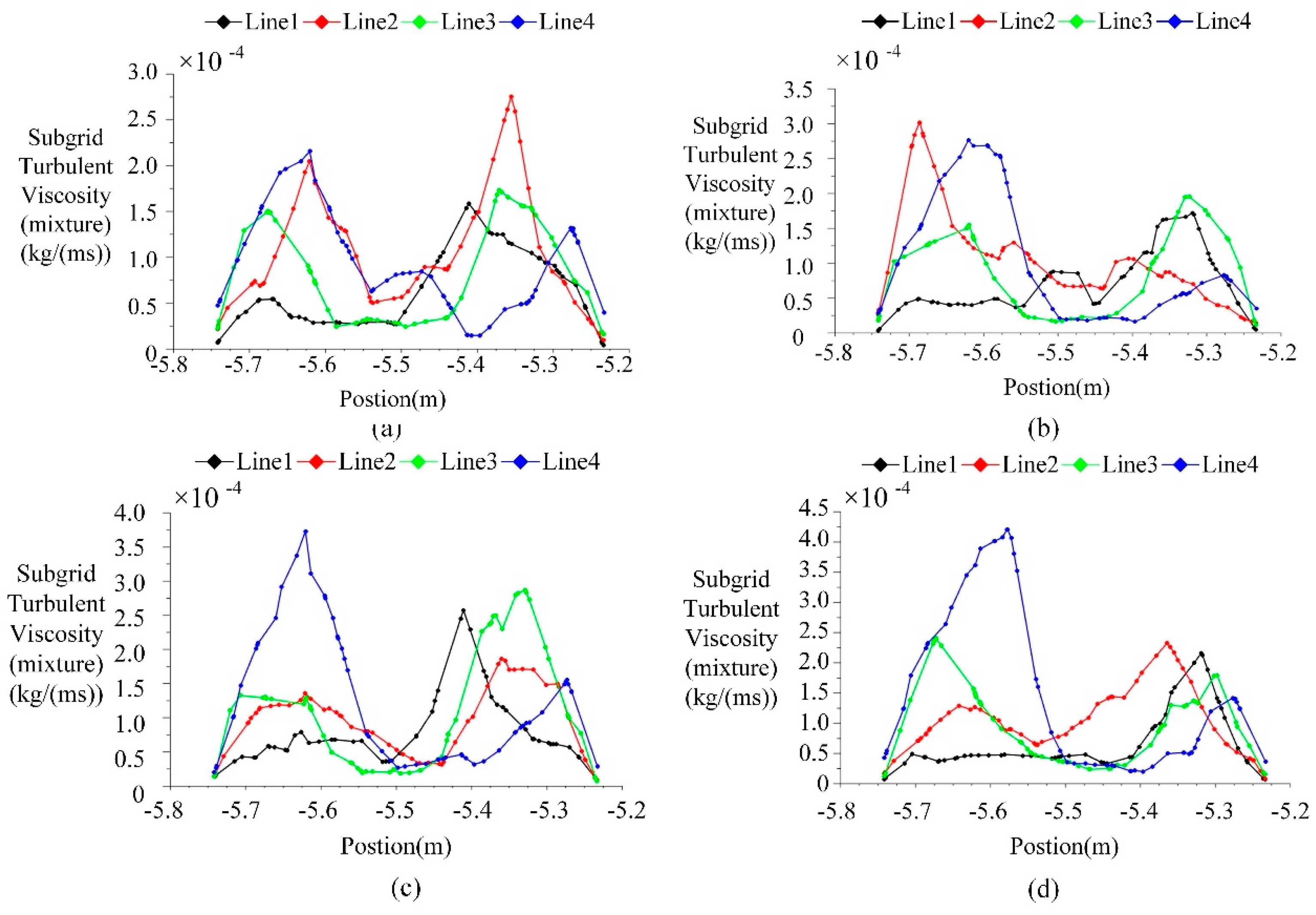
The turbulent viscosity curves at different locations have been obtained, as depicted in Figure 12. It is observed that at branches 1–3, despite differences in turbulent viscosity on both sides of the pipeline at different locations, the distribution of turbulent viscosity on both sides becomes more uniform over time. At the junction of branch 4, the maximum turbulent viscosity on the lower side of the bend can reach 4.0 × 10⁻⁴ kg/(m·s), indicating that the structure on the lower side of the bend causes more excellent turbulent viscous resistance near the wall, leading to complex turbulent vortex coupling and a banded distribution of turbulence energies at walls. When mixing fluids are in stable development states, flow characteristics after the intermixing of the eight branches become uniform. However, the design of the bend makes the flow evolution process complex, significantly influencing the slug flow generation.
4.4. Gas Content of the Pipe Slug Flows
In order to study the complex flow characteristics of pipeline slug flow, the evolution process of gas content with time series was obtained, as shown in Figure 13. At the initial moment, the pipe is filled with gas, and the volume fraction of the gas content is 1. As the gas and liquid flow into the pipe from the inlet, the volume fraction of the gas phase decreases continuously until its value is 0. At this time, the fluid in the pipeline is all liquid phase. With the coupling of gas and liquid, slug phenomenon is constantly formed inside the riser, resulting in periodic changes in gas content. At this time, the gas is continuously pumped into the riser, pushing the slug to flow upward, and the gas content inside the pipeline increases to 0.475, and then decreases to 0. Under the action of gas phase, the slug inside the pipeline flows to the top of the riser and exits the riser. Subsequently, a new slug phenomenon was formed inside the pipeline under the action of gas–liquid coupling. Therefore, if you want to avoid the occurrence of slug phenomenon, reasonable design of pipeline structure is very important.
From the above phenomena, it can be inferred that the gas–liquid coupling process of mixed fluid at the intersection of horizontal pipe A and vertical pipe B is easy to form a complex slug flow phenomenon, which has strong nonlinear evolution characteristics and complex changes in the size and shape of the slug. The gas–liquid two-phase fluid in the riser flows upward under the action of the slug, forming a serious slug flow phenomenon. When the flow rate in the pipeline is large, the gas–liquid coupling process is accelerated, which increases the formation speed of the pipeline slug flow, and inevitably intensifies the morphology evolution process of the pipeline slug flow. In general, pipeline slug flow is a complicated turbulent mechanical phenomenon. How to optimize the design of pipeline system to avoid the formation of slug flow is of great significance.
5. Conclusions
Gas–liquid slug flows are widespread in marine, oil, and chemical industries, and it is vital to study the formation mechanism and flow patterns of slug flows. This paper establishes a gas–liquid slug flow model with multiple inlets, obtaining the dynamics of complex pipeline flow.
- Due to the counterflow course, bias flow phenomena occur in the initial evolution of gas-phase volume fraction distribution. When the flow field evolves, mixing process becomes uniform, resulting in optimal mixing throughout the flow field.
- Due to the intermittent characteristics of the liquid plug, there is no apparent bias in upper and lower branch pipelines. That is, slug flow will not be biased under symmetrical pipelines. The pressure drop fluctuation of horizontal and vertical pipe is strong, which is related to the gas–liquid slug flow.
- For the multi-inlet pipeline model, a specific deviation exists at the junctions of the first three sets of branch pipes, with a low-speed area near the pipeline wall, causing an uneven distribution of components on both sides of the pipeline. The fluid flow velocity is uneven at the end of the fourth branch pipe junction, with a noticeable bias flow phenomenon.
- The turbulence viscosity inside the pipeline is influenced by the viscous resistance of the walls and is distributed along the pipeline wall. The turbulence viscosity distribution is relatively uniform at each branch pipe junction. However, the design of the bent pipe structure results in an unbalanced flow velocity distribution and turbulence viscosity on both sides of the pipeline, exhibiting a banded distribution characteristic.
Author Contributions
Conceptualization, Q.Y. and D.L.; article identification, selection, and analysis, Q.Y. and K.W.; tables and figures generation, Q.Y.; writing—original draft preparation, Q.Y.; funding acquisition, Q.Y., D.L. and G.Z.; review and editing, Q.Y., K.W. and G.Z.; formal analysis and investigation, Q.Y. All authors have read and agreed to the published version of the manuscript.
Funding
This work was partly supported by the Zhejiang Soft Science Research Program Project (2024C35116); National and Regional Research Project on German Speaking Countries of Zhejiang University of Science and Technology (2023DEGB009); Fundamental Research Funds for the Provincial Universities of Zhejiang University of Science and Technology under Grant No. 2023QN041.
Data Availability Statement
The data presented in this study are available on request from the corresponding author.
Conflicts of Interest
Author Kefu Wang was employed by the company Zhejiang Qiaoshi Intelligent Industry Co., Ltd. The remaining authors declare that the research was conducted in the absence of any commercial or financial relationships that could be construed as a potential conflict of interest.
References
- Li, Y.C.; Hosseini, M.; Arasteh, H. Transition simulation of two-phase intermittent slug flow characteristics in oil and gas pipelines. Int. Commun. Heat Mass Transf. 2020, 113, 104534. [Google Scholar] [CrossRef]
- Li, Q.H.; Xu, P.; Li, L.; Xu, W.X.; Tan, D.P. Investigation on the lubrication heat transfer mechanism of the multilevel gearbox by the lattice boltzmann method. Processes 2024, 12, 381. [Google Scholar] [CrossRef]
- Chen, J.T.; Ge, M.; Li, L.; Zheng, G. Material transport and flow pattern characteristics of gas–liquid–solid mixed flows. Processes 2023, 11, 2254. [Google Scholar] [CrossRef]
- Mou, M.Y.; dela Rosa, L. Continuous Generation of Gas-Water Slugs with Improved Size Uniformity at a Tunable Scale. Chem. Eng. Technol. 2023, 46, 2073–2080. [Google Scholar] [CrossRef]
- Li, L.; Li, Q.H.; Ni, Y.S.; Wang, C.Y.; Tan, Y.F.; Tan, D.P. Critical penetrating vibration evolution behaviors of the gas-liquid coupled vortex flow. Energy 2024, 292, 130236. [Google Scholar] [CrossRef]
- Tan, D.P.; Li, L.; Zhu, Y.L.; Zheng, S.; Yin, Z.C.; Li, D. Critical penetration condition and Ekman suction-extraction mechanism of a sink vortex. J. Zhejiang Univ.-SCI A. 2019, 20, 61–72. [Google Scholar] [CrossRef]
- Liu, Z.B.; Wang, S.; Chen, Z.R. Evaluation of Slug Flow-Induced Flexural Loading in Pipelines Using a Surrogate Model. J. Offshore Mech. Arct. Eng. -Trans. ASME 2013, 135, 031703. [Google Scholar]
- Reda, A.; Forbes, G.L.; Sultan, I.A.; Howard, I.M. Pipeline Slug Flow Dynamic Load Characterization. J. Offshore Mech. Arct. Eng. -Trans. ASME 2019, 141, 0117011. [Google Scholar] [CrossRef]
- Yin, Z.C.; Ni, Y.S.; Li, L.; Wang, T.; Wu, J.F.; Li, Z.; Tan, D.P. Numerical modelling and experimental investigation of a two-phase sink vortex and its fluid-solid vibration characteristics. J. Zhejiang Univ.-SCI A. 2024, 25, 47–62. [Google Scholar] [CrossRef]
- Tastan, K.; Erat, B.; Barbaros, E.; Eroglu, N. Flow boundary effects on scour characteristics upstream of pipe intakes. Ocean Eng. 2023, 278, 114343. [Google Scholar] [CrossRef]
- Eyo, E.N.; Lao, L.Y. Slug flow characterization in horizontal annulus. AICHE J. 2019, 65, e16711. [Google Scholar] [CrossRef]
- Qu, Z.G.; Jin, S.; Wu, L.Q.; An, Y.; Liu, Y.; Fang, R.; Tang, J. Influence of water flow velocity on fouling removal for pipeline based on eco-friendly ultrasonic guided wave technology. J. Clean. Prod. 2019, 240, 118173. [Google Scholar] [CrossRef]
- Liu, L.; Zhang, X.T.; Tian, X.L.; Li, X. Numerical investigation on dynamic performance of vertical hydraulic transport in deepsea mining. Appl. Ocean Res. 2023, 130, 103443. [Google Scholar] [CrossRef]
- Sun, Z.; Yao, Q.; Jin, H.; Xu, Y.; Hang, W.; Chen, H.; Li, K.; Shi, L.; Gu, J.; Zhang, Q.; et al. A novel in-situ sensor calibration method for building thermal systems based on virtual samples and autoencoder. Energy 2024, in press. [Google Scholar]
- Ho, Y.; Song, L.; Liu, Z.; Yao, J. Identification of ship hydrodynamic derivatives based on LS-SVM with wavelet threshold denoising. J. Mar. Sci. Eng. 2021, 9, 1356. [Google Scholar] [CrossRef]
- Tamburini, A.; Cipollina, A.; Micale, G. CFD simulations of dense solid-liquid suspensions in baffled stirred tanks: Prediction of the minimum impeller speed for complete suspension. Chem. Eng. J. 2012, 193, 234–255. [Google Scholar] [CrossRef]
- Wu, J.F.; Li, L.; Li, Z.; Wang, T.; Tan, Y.F.; Tan, D.P. Mass transfer mechanism of multiphase shear flows and interphase optimization solving method. Energy 2024, 292, 130475. [Google Scholar] [CrossRef]
- Son, J.H.; Sohn, C.H.; Park, I.S. Numerical study of 3-D air core phenomenon during liquid draining. J. Mech. Sci. Technol. 2015, 29, 4247–4257. [Google Scholar] [CrossRef]
- Zhao, Y.Z.; Gu, Z.L.; Yu, Y.Z.; Li, Y.; Feng, X. Numerical analysis of structure and evolution of free water vortex. J. Xi’an Jiaotong Univ. 2003, 37, 85–88. [Google Scholar]
- Fan, Y.L.; Pereyra, E.; Sarica, C. Experimental study of pseudo-slug flow in upward inclined pipes. J. Nat. Gas Sci. Eng. 2020, 75, 103147. [Google Scholar] [CrossRef]
- Li, L.; Yang, Y.S.; Xu, W.X.; Lu, B.; Gu, Z.H.; Yang, J.G.; Tan, D.P. Advances in the multiphase vortex-induced vibration detection method and its vital technology for sustainable industrial production. Appl. Sci. 2022, 12, 8538. [Google Scholar] [CrossRef]
- Liu, Y.; Wang, S. Distribution of gas-liquid two-phase slug flow in parallel micro-channels with different branch spacing. Int. J. Heat Mass Transf. 2019, 132, 606–617. [Google Scholar] [CrossRef]
- Li, L.; Tan, Y.F.; Xu, W.X.; Ni, Y.S.; Yang, J.G.; Tan, D.P. Fluid-induced transport dynamics and vibration patterns of multiphase vortex in the critical transition states. Int. J. Mech. Sci. 2023, 252, 108376. [Google Scholar] [CrossRef]
- Pineda-Pérez, H.; Kim, T.; Pereyra, E.; Ratkovich, N. CFD modeling of air and highly viscous liquid two-phase slug flow in horizontal pipes. Chem. Eng. Res. Des. 2018, 136, 638–653. [Google Scholar] [CrossRef]
- Schmelter, S.; Olbrich, M.; Schmeyer, E.; Bär, M. Numerical simulation, validation, and analysis of two-phase slug flow in large horizontal pipes. Flow Meas. Instrum. 2020, 73, 101722. [Google Scholar] [CrossRef]
- Tan, Y.F.; Ni, Y.S.; Xu, W.X.; Xie, Y.S.; Li, L.; Tan, D.P. Key technologies and development trends of the soft abrasive flow finishing method. J. Zhejiang Univ. -Sci. A. 2023, 24, 1043–1064. [Google Scholar] [CrossRef]
- Lu, J.F.; Wang, T.; Li, L.; Yin, Z.C. Dynamic Characteristics and Wall Effects of Bubble Bursting in Gas-Liquid-Solid Three-Phase Particle Flow. Processes 2020, 8, 760. [Google Scholar] [CrossRef]
- Li, L.; Xu, W.X.; Tan, Y.F.; Yang, Y.S.; Yang, J.G.; Tan, D.P. Fluid-induced vibration evolution mechanism of multiphase free sink vortex and the multi-source vibration sensing method. Mech. Syst. Signal Process. 2023, 189, 110058. [Google Scholar] [CrossRef]
- Kim, H.S.; Kim, B.W.; Lee, K.; Sung, H.G. Application of Average Sea-state Method for Fast Estimation of Fatigue Damage of Offshore Structure in Waves with Various Distribution Types of Occurrence Probability. Ocean Eng. 2022, 246, 110601. [Google Scholar] [CrossRef]
- Zheng, G.A.; Gu, Z.H.; Xu, W.X.; Li, Q.H.; Tan, Y.F.; Wang, C.Y.; Li, L. Gravitational surface vortex formation and suppression control: A review from hydrodynamic characteristics. Processes 2023, 11, 42. [Google Scholar] [CrossRef]
- Ge, M.; Zheng, G.A. Fluid-solid mixing transfer mechanism and flow patterns of the double-layered impeller stirring tank by the CFD-DEM method. Energies 2024, 17, 1513. [Google Scholar] [CrossRef]
- Al-Safran, E. Investigation and prediction of slug frequency in gas/liquid horizontal pipe flow. J. Pet. Sci. Eng. 2009, 69, 143–155. [Google Scholar] [CrossRef]
- Zheng, G.A.; Shi, J.L.; Li, L.; Li, Q.H.; Gu, Z.H.; Xu, W.X.; Lu, B. Fluid-solid coupling-based vibration generation mechanism of the multiphase vortex. Processes 2023, 11, 568. [Google Scholar] [CrossRef]
- Zheng, G.A.; Xu, P.; Li, L.; Fan, X.H. Investigations of the Formation Mechanism and Pressure Pulsation Characteristics of Pipeline Gas-Liquid Slug Flows. J. Mar. Sci. Eng. 2024, in press. [Google Scholar]
- Khishe, M. Drw-ae: A deep recurrent-wavelet autoencoder for underwater target recognition. IEEE J. Ocean. Eng. 2022, 47, 1083–1098. [Google Scholar] [CrossRef]
- Li, L.; Gu, Z.H.; Xu, W.X.; Tan, Y.F.; Fan, X.H.; Tan, D.P. Mixing mass transfer mechanism and dynamic control of gas–liquid–solid multiphase flow based on VOF-DEM coupling. Energy 2023, 272, 127015. [Google Scholar] [CrossRef]
- Ruponen, P.; Manderbacka, T.; Lindroth, D. On the Calculation of the Righting Lever Curve for a Damaged Ship. Ocean Eng. 2018, 149, 313–324. [Google Scholar] [CrossRef]
- Han, Y.; Cundall, P.A. LBM-DEM modeling of fluid-solid interaction in porous media. Int. J. Numer. Anal. Methods Geomech. 2013, 37, 1391–1407. [Google Scholar] [CrossRef]
- Li, L.; Qi, H.; Yin, Z.C.; Li, D.F.; Zhu, Z.L.; Tangwarodomnukun, V.; Tan, D.P. Investigation on the multiphase sink vortex Ekman pumping effects by CFD-DEM coupling method. Powder Technol. 2020, 360, 462–480. [Google Scholar] [CrossRef]
- Li, L.; Lu, B.; Xu, W.X.; Wang, C.Y.; Wu, J.F.; Tan, D.P. Dynamic behaviors of multiphase vortex-induced vibration for hydropower energy conversion. Energy 2024, in press. [Google Scholar]
- Woods, B.D.; Fan, Z.; Hanratty, T.J. Frequency and development of slugs in a horizontal pipe at large liquid flows. Int. J. Multiph. Flow 2006, 32, 902–925. [Google Scholar] [CrossRef]
- Lin, L.; Tan, D.P.; Yin, Z.C.; Wang, T.; Fan, X.H.; Wang, R.H. Investigation on the multiphase vortex and its fluid-solid vibration characters for sustainability production. Renew. Energy 2021, 175, 887–909. [Google Scholar]
- Ezure, T.; Ito, K.; Tanaka, M.; Ohshima, H.; Kameyama, Y. Experiments on gas entrainment phenomena due to free surface vortex induced by flow passing beside stagnation region. Nucl. Eng. Des. 2019, 350, 90–97. [Google Scholar] [CrossRef]
- Zheng, D.; Che, D. Experimental study on hydrodynamic characteristics of upward gas–liquid slug flow. Int. J. Multiph. Flow 2006, 32, 1191–1218. [Google Scholar] [CrossRef]
- Li, L.; Tan, D.P.; Wang, T.; Yin, Z.C.; Fan, X.H.; Wang, R.H. Multiphase coupling mechanism of free surface vortex and the vibration-based sensing method. Energy 2021, 216, 119136. [Google Scholar] [CrossRef]
- Yan, Q.; Fan, X.H.; Li, L.; Zheng, G.A. Investigations of the mass transfer and flow field disturbance regulation of the gas–liquid–solid flow of hydropower stations. J. Mar. Sci. Eng. 2024, 12, 84. [Google Scholar] [CrossRef]
- Wan, Z.H.; Yang, S.L.; Hu, J.H.; Wang, H. Multiphysics coupling investigation of interphase heat transfer in gas-particle coaxial-jet mixing flow via CFD-DEM-CHT. Chem. Eng. J. 2023, 465, 142870. [Google Scholar] [CrossRef]
- Tan, Y.F.; Ni, Y.S.; Wu, J.F.; Li, L.; Tan, D.P. Machinability evolution of gas-liquid-solid three-phase rotary abrasive flow finishing. Int. J. Adv. Manuf. Technol. 2023, 131, 2145–2164. [Google Scholar] [CrossRef]
- Li, L.; Lu, J.F.; Fang, H.; Yin, Z.C.; Wang, T.; Wang, R.H.; Fan, X.H.; Zhao, L.J.; Tan, D.P.; Wan, Y.H. Lattice Boltzmann method for fluid-thermal systems: Status, hotspots, trends and outlook. IEEE Access 2020, 8, 27649–27675. [Google Scholar] [CrossRef]
- Xiao, F.; Luo, M.; Huang, F.Y. CFD-DEM investigation of gas-solid flow and wall erosion of vortex elbows conveying coarse particles. Powder Technol. 2023, 424, 118524. [Google Scholar] [CrossRef]
- Fan, H.C.; Hou, Q.Z. Mass shedding rate of an isolated high-speed slug propagating in a pipeline. Eng. Appl. Comput. Fluid Mech. 2024, 18, 2303372. [Google Scholar] [CrossRef]
- Yin, Z.C.; Lu, J.F.; Li, L.; Wang, T.; Wang, R.H.; Fan, X.H.; Lin, H.K.; Huang, Y.S.; Tan, D.P. Optimized Scheme for Accelerating the Slagging Reaction and Slag-Metal-Gas Emulsification in a Basic Oxygen Furnace. Appl. Sci. 2020, 10, 5101. [Google Scholar] [CrossRef]
- Che, H.Q.; Werner, D.; Seville, J. Evaluation of coarse-grained CFD-DEM models with the validation of PEPT measurement. Particuology 2023, 82, 48–63. [Google Scholar] [CrossRef]
- Li, L.; Lu, B.; Xu, W.X.; Gu, Z.H.; Yang, Y.S.; Tan, D.P. Mechanism of multiphase coupling transport evolution of free sink vortex. Acta Phys. Sin. 2023, 72, 034702. [Google Scholar] [CrossRef]
- Papanikolaou, A.; Xing-Kaeding, Y.; Strobel, J.; Kanellopoulou, A.; Zaraphonitis, G.; Tolo, E. Numerical and Experimental Optimization Study on a Fast, Zero Emission Catamaran. J. Mar. Sci. Eng. 2020, 8, 657. [Google Scholar] [CrossRef]
- Tan, D.P.; Li, L.; Li, D.F.; Zhu, Y.L.; Zheng, S. Ekman boundary layer mass transfer mechanism of free sink vortex. Int. J. Heat Mass Transf. 2020, 150, 119250. [Google Scholar] [CrossRef]
- Metallinos, A.S.; Repousis, E.G.; Memos, C.D. Wave Propagation over a Submerged Porous Breakwater with Steep Slopes. Ocean Eng. 2016, 111, 424–438. [Google Scholar] [CrossRef]
- Wang, T.; Li, L.; Yin, Z.C.; Xie, Z.W.; Wu, J.F.; Zhang, Y.C.; Tan, D.P. Investigation on the flow field regulation characteristics of the right-angled channel by impinging disturbance method. Proc. Inst. Mech. Eng. Part C J. Mech. Eng. Sci. 2022, 236, 11196–11210. [Google Scholar] [CrossRef]
- Wang, T.; Wang, C.Y.; Yin, Z.C.; Zhang, Y.K.; Li, L.; Tan, D.P. Analytical approach for nonlinear vibration response of the thin cylindrical shell with a straight crack. Nonlinear Dyn. 2023, 111, 10957–10980. [Google Scholar] [CrossRef]
- Liu, B.; Villavicencio, R.; Pedersen, P.T.; Guedes Soares, C. Analysis of structural crashworthiness of double-hull ships in collision and grounding. Mar. Struct. 2021, 76, 102898. [Google Scholar] [CrossRef]
Figure 1.
Geometric model of multi-entrance pipelines.

Figure 2.
Numerical model of gas–liquid slug flows.

Figure 3.
Volume fraction cloud pictures of the gas phase. (a) t = 5 s. (b) t = 10 s. (c) t = 15 s. (d) t = 20 s. (e) t = 25 s. (f) t = 30 s.
Figure 3.
Volume fraction cloud pictures of the gas phase. (a) t = 5 s. (b) t = 10 s. (c) t = 15 s. (d) t = 20 s. (e) t = 25 s. (f) t = 30 s.

Figure 4.
Shunt characteristics of gas–liquid slug flows.

Figure 5.
Flow characteristics in intersection pipes.

Figure 6.
Evolution curve of pipeline pressure drops with time.

Figure 7.
Distribution of detection points at different locations.

Figure 8.
Gas-phase volume fraction at different locations. (a) t = 20 s. (b) t = 25 s. (c) t = 30 s. (d) t = 35 s.
Figure 8.
Gas-phase volume fraction at different locations. (a) t = 20 s. (b) t = 25 s. (c) t = 30 s. (d) t = 35 s.

Figure 9.
Velocity contour maps of the fluid. (a) t = 20 s. (b) t = 25 s. (c) t = 30 s. (d) t = 35 s.
Figure 9.
Velocity contour maps of the fluid. (a) t = 20 s. (b) t = 25 s. (c) t = 30 s. (d) t = 35 s.

Figure 10.
Fluid velocity curves at different locations. (a) t = 20 s. (b) t = 25 s. (c) t = 30 s. (d) t = 35 s.
Figure 10.
Fluid velocity curves at different locations. (a) t = 20 s. (b) t = 25 s. (c) t = 30 s. (d) t = 35 s.

Figure 11.
Turbulent viscosity cloud maps. (a) t = 20 s. (b) t = 25 s. (c) t = 30 s. (d) t = 35 s.

Figure 12.
Turbulent viscosity curves at different locations. (a) t = 20 s. (b) t = 25 s. (c) t = 30 s. (d) t = 35 s.
Figure 12.
Turbulent viscosity curves at different locations. (a) t = 20 s. (b) t = 25 s. (c) t = 30 s. (d) t = 35 s.

Figure 13.
Evolution of gas content in pipelines.


Table 1.
Grid independence validation.
| Model | Grid Quantity | Pmax (kPa) | Pmin (kPa) | Pamp (kPa) |
|---|---|---|---|---|
| Model 1 | 689,054 | 46.67 | 5.45 | 41.04 |
| Model 2 | 806,590 | 47.19 | 5.58 | 41.61 |
| Model 3 | 952,580 | 47.63 | 5.64 | 41.99 |
| Minimum relative error (%) | / | 0.92 | 1.1 | 0.90 |
Disclaimer/Publisher’s Note: The statements, opinions and data contained in all publications are solely those of the individual author(s) and contributor(s) and not of MDPI and/or the editor(s). MDPI and/or the editor(s) disclaim responsibility for any injury to people or property resulting from any ideas, methods, instructions or products referred to in the content. |
© 2024 by the authors. Licensee MDPI, Basel, Switzerland. This article is an open access article distributed under the terms and conditions of the Creative Commons Attribution (CC BY) license (https://creativecommons.org/licenses/by/4.0/).
Share and Cite
MDPI and ACS Style
Yan, Q.; Li, D.; Wang, K.; Zheng, G. Study on the Hydrodynamic Evolution Mechanism and Drift Flow Patterns of Pipeline Gas–Liquid Flow. Processes 2024, 12, 695. https://0-doi-org.brum.beds.ac.uk/10.3390/pr12040695
AMA Style
Yan Q, Li D, Wang K, Zheng G. Study on the Hydrodynamic Evolution Mechanism and Drift Flow Patterns of Pipeline Gas–Liquid Flow. Processes. 2024; 12(4):695. https://0-doi-org.brum.beds.ac.uk/10.3390/pr12040695
Chicago/Turabian StyleYan, Qing, Donghui Li, Kefu Wang, and Gaoan Zheng. 2024. "Study on the Hydrodynamic Evolution Mechanism and Drift Flow Patterns of Pipeline Gas–Liquid Flow" Processes 12, no. 4: 695. https://0-doi-org.brum.beds.ac.uk/10.3390/pr12040695
Note that from the first issue of 2016, this journal uses article numbers instead of page numbers. See further details here.