Waterwheel Plant Algorithm: A Novel Metaheuristic Optimization Method

Abstract

Attempting to address optimization problems in various scientific disciplines is a fundamental and significant difficulty requiring optimization. This study presents the waterwheel plant technique (WWPA), a novel stochastic optimization technique motivated by natural systems. The proposed WWPA’s basic concept is based on modeling the waterwheel plant’s natural behavior while on a hunting expedition. To find prey, WWPA uses plants as search agents. We present WWPA’s mathematical model for use in addressing optimization problems. Twenty-three objective functions of varying unimodal and multimodal types were used to assess WWPA’s performance. The results of optimizing unimodal functions demonstrate WWPA’s strong exploitation ability to get close to the optimal solution, while the results of optimizing multimodal functions show WWPA’s strong exploration ability to zero in on the major optimal region of the search space. Three engineering design problems were also used to gauge WWPA’s potential for improving practical programs. The effectiveness of WWPA in optimization was evaluated by comparing its results with those of seven widely used metaheuristic algorithms. When compared with eight competing algorithms, the simulation results and analyses demonstrate that WWPA outperformed them by finding a more proportionate balance between exploration and exploitation.

1. Introduction

Optimization is finding the optimal settings for a system’s design parameters to minimize or maximize the fitness function. At the same time, all of the constraints are met [1,2]. Optimization difficulties exist in every industry, academic discipline, and study area. Exact algorithms are one type of optimization strategy, whereas heuristic and metaheuristic algorithms are another [3,4,5]. Because it requires fewer sophisticated calculations, the former category takes less time to complete, but it may be less useful and practical. As opposed to the former, the second class of algorithms (metaheuristics) exhibits some random/stochastic behavior and makes an “informed search choice” for some “wise areas” [6].

The above theorem inspires scientists to develop cutting-edge algorithms and improve existing ones. Since optimization exists in many disciplines, including cloud computing activities [7], face identification [8], power [9,10], and engineering challenges [11], it has recently attracted a lot of attention from researchers. According to the No Free Lunch (NFL) hypothesis [12], no algorithm can identify the best solution in all cases, and many optimization algorithms have been published. In other words, an algorithm that succeeds in finding the best answer to one kind of problem does not succeed in solving another.

Because metaheuristic algorithms use a form of random search, it is impossible to guarantee that they always find the global optimum. However, due to their closeness to the global optimal solution, metaheuristic algorithms’ solutions are regarded as quasi-optimal [13]. To find a workable answer, metaheuristic algorithms need strong search capabilities in both global and local problem-solving spaces. Combining exploration with the global search process may improve the algorithm’s capacity to find the primary optimum region and break out of local optima. The algorithm’s capacity to converge on potentially superior solutions in promising areas is improved by the search process at the local level, which incorporates the idea of exploitation [14]. While searching for an optimal solution, metaheuristic algorithms thrive when they balance exploration and exploitation. Thus, an algorithm that better balances exploration and exploitation when comparing the performance of many metaheuristic algorithms on an optimization problem [15] provides a better quasi-optimal solution. Many metaheuristic algorithms have been developed to improve the quality of results obtained for optimization problems.

Optimization methods can be categorized as either deterministic or stochastic. Solving linear, convex, continuous, differentiable, and low-dimensional optimization problems is applicable within the capabilities of both gradient-based and non-gradient-based deterministic techniques [16]. Optimization problems that are non-linear, non-convex, discontinuous, non-differentiable, and/or high-dimensional are unfortunately outside the scope of deterministic techniques. Deterministic methods provide bad results in this optimization problem, because they become mired in local optimum solutions [17].

Optimizing problems are notoriously challenging to solve using deterministic methods; thus, academics have responded to stochastic processes. An effective random search in the problem-solving space employing random operators and trial-and-error procedures characterizes metaheuristic algorithms, one of the most popular stochastic approaches [18]. Metaheuristic algorithms have gained popularity for handling optimization problems due to their effectiveness in solving problems that are non-linear, non-convex, discontinuous, non-differentiable, NP-hard, complex, and high-dimensional. They also require no differentiable information about the objective function or constraints and are not dependent on the problem type [19].

Considering the many metaheuristic algorithms that have already been developed, whether there is still a need to introduce even more metaheuristic algorithms is the key question that drives metaheuristic algorithm research. The NFL theorem [20] answers this topic by showing that there is no universally superior metaheuristic method for optimization. Even if a metaheuristic algorithm addresses one set of optimization problems, it does not mean that it works just as well for solving another set of optimization problems. The NFL theorem states that an algorithm may succeed in addressing one optimization problem while failing to solve a different one. So, when applied to optimization problems, a metaheuristic algorithm’s output may be taken at face value. As a result, the NFL theorem motivates researchers to create cutting-edge metaheuristic algorithms that can more efficiently solve optimization problems.

This paper’s innovative contribution is the design of a new metaheuristic algorithm for addressing optimization problems in various scientific disciplines; the method is called Waterwheel Plant Algorithm (WWPA). The following are the most significant contributions of this work:

• Modeling natural waterwheel behavior inspired the development of WWPA.
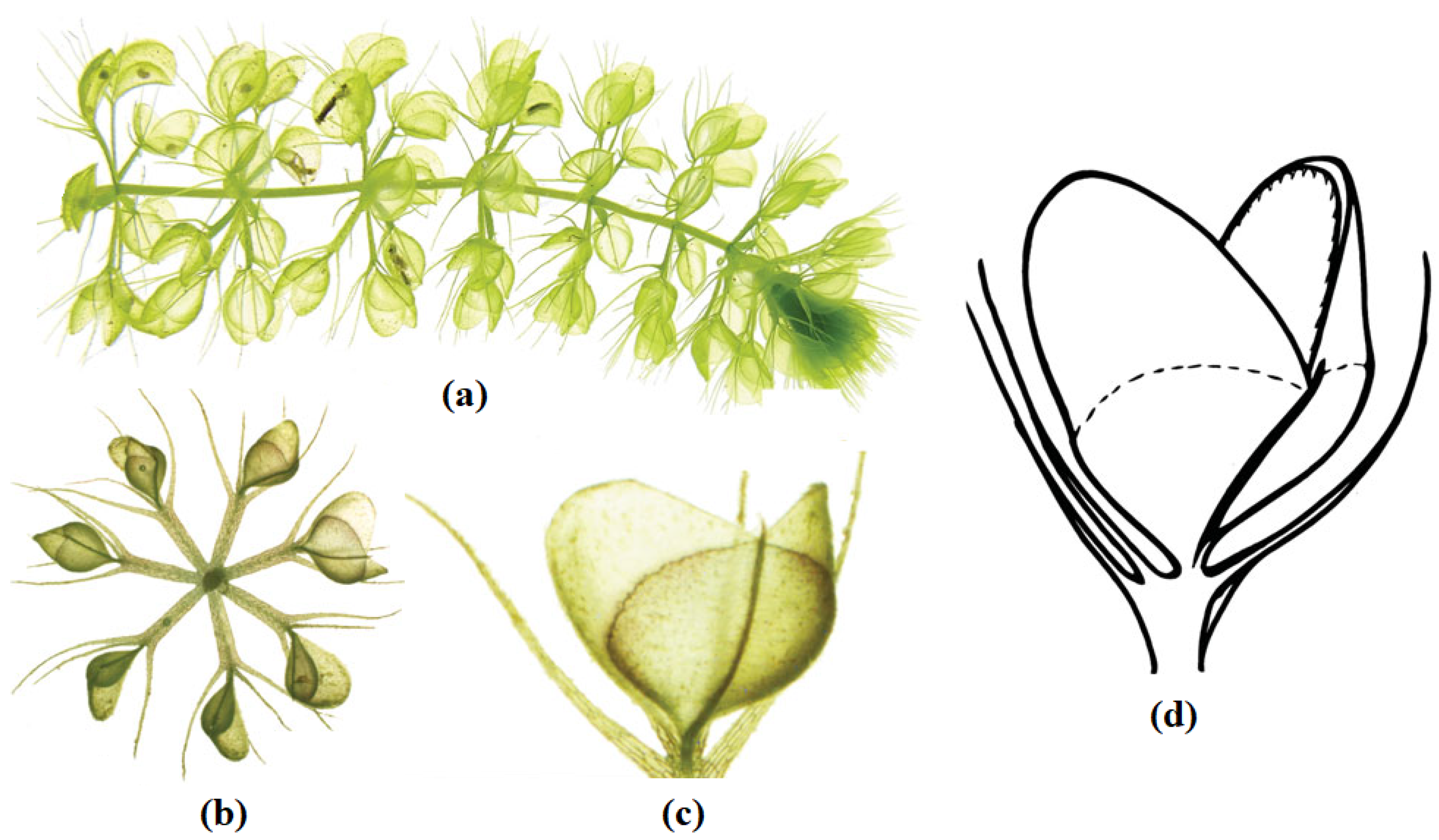
• The method used by waterwheel plants to locate their insect food, capture it, and then move it to a more convenient location before devouring it inspired the essential idea of WWPA.
• We provide a mathematical model of the WWPA implementation processes throughout the two exploration and exploitation stages.
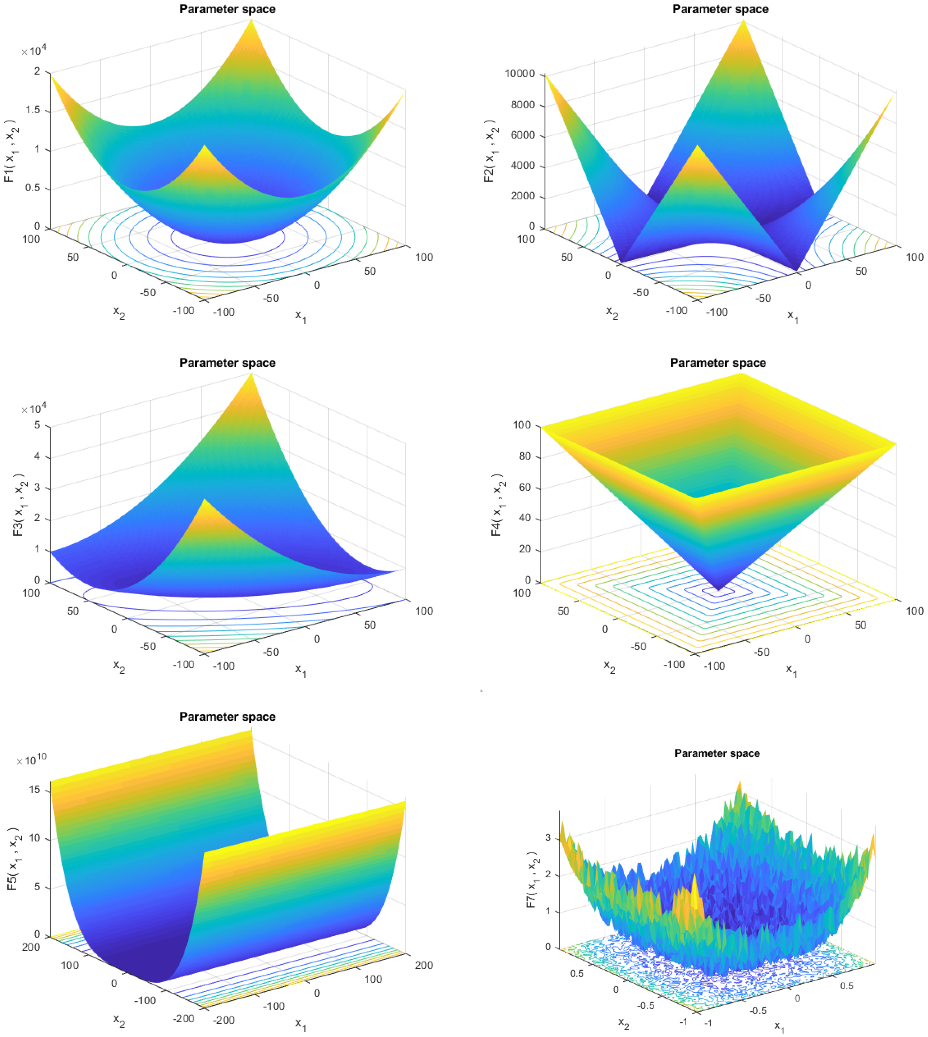
• Twenty-three benchmark functions were used to measure WWPA’s efficiency in various optimization tasks.
• Three engineering problems were considered in evaluating the effectiveness of the proposed WWPA.
• Well-known algorithms were used as benchmarks against which the proposed WWPA method was evaluated.
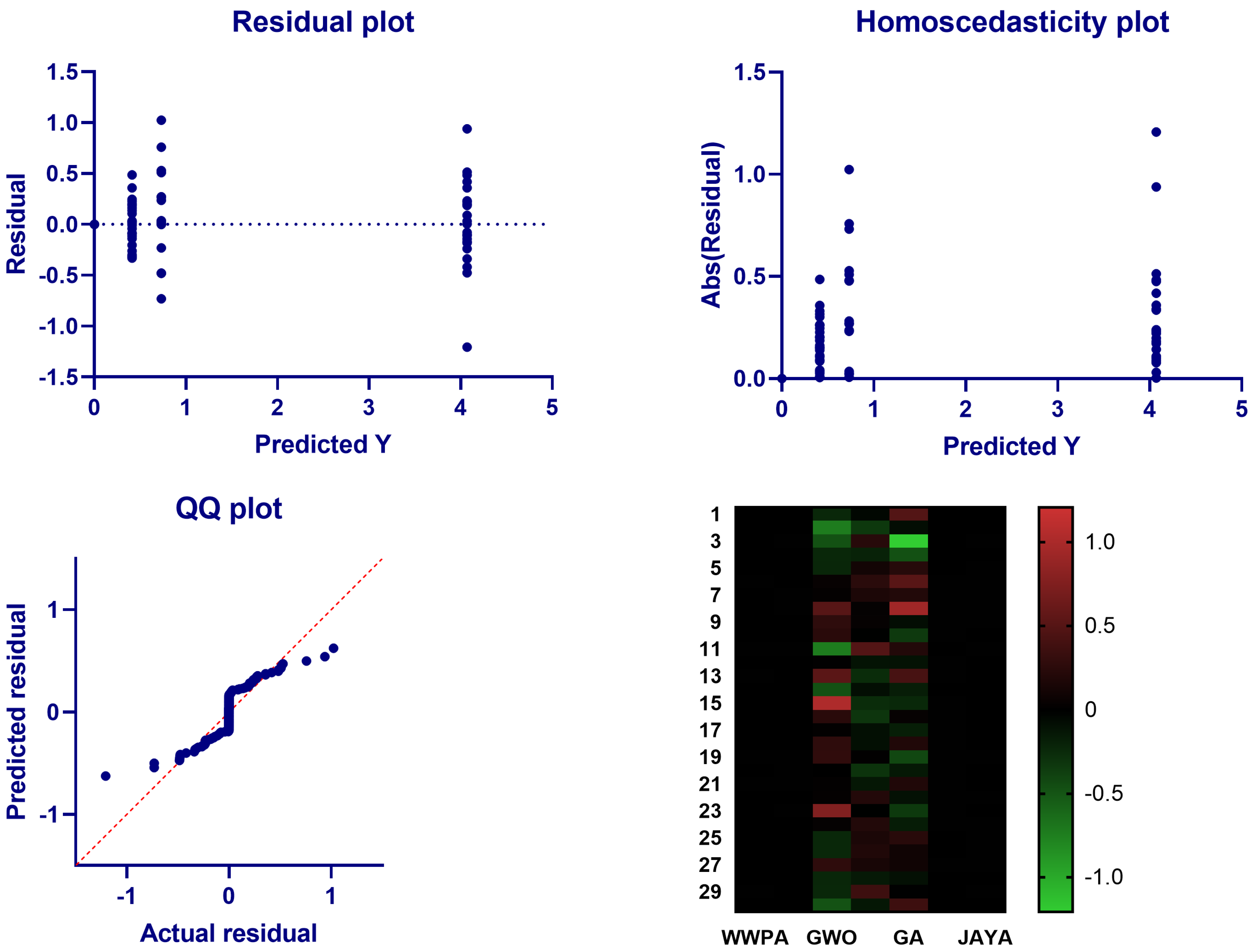
• A statistical analysis was performed to confirm the significant difference of the proposed approach when compared with the other competitor algorithms.

The following is how the rest of the paper is laid out: In Section 2, we present our literature review. Section 3 then presents the mathematical model and the introduction to the proposed Waterwheel Plant Algorithm (WWPA). Simulation and effectiveness studies for optimization problems in addition to the assessment of how well the proposed WWPA performed in handling practical problems are then described in Section 4. Section 5 summarizes the results, and suggestions for further research are offered.

2. Literature Review

When dealing with practical problems, it is common to encounter a large number of local optimum solutions, since the search space is typically complicated. An optimization method is more likely to converge too quickly because of this, leading to an increased risk of local optimizations. Many optimization algorithms attempt to address this problem by employing methods that broaden the population’s genetic makeup. Local optima may be avoided by using these methods, although the convergence performance may suffer. Consequently, creating a powerful metaheuristic algorithm for optimization necessitates striking a balance between exploration and exploitation. As a result of striking this equilibrium, the optimization algorithm’s convergence speed is enhanced, and the search space is explored more thoroughly, allowing the local optima to be avoided. Metaheuristic algorithms draw inspiration from various sources, including evolutionary occurrences, natural phenomena, animal life in nature, biological sciences, physics, game rules, and human relationships.

Natural swarming phenomena, such as those seen in insects, fish, birds, mammals, and plants and animals, have inspired the development of new metaheuristic algorithms that use swarm intelligence to solve problems. Metaheuristic algorithms can be categorized into five classes based on the type of motivation employed in their development: swarm-based, evolutionary-based, physics-based, human-based, and game-based. The most well-known swarm-based algorithms include Particle Swarm Optimization (PSO) [21], Ant Colony Optimization (ACO) [22], and Artificial Bee Colony (ABC) [23,24]. The PSO design is based on the analogy of animal flocks foraging for food. The ability of ants to find the quickest route from their colony to a food supply significantly influenced the development of ACO. The design of ABC is based on a simulation of the behavior of foraging bee colonies. Swarm-based algorithms include Golden Jackal Optimization (GJO) [25], Coati Optimization Algorithm (COA) [26], Marine Predator Algorithm (MPA) [27], and Mountain Gazelle Optimizer (MGO) [28].

The biological sciences, genetics, Darwin’s theory of evolution, survival of the fittest, and natural selection inspired the development of evolutionary-based metaheuristic algorithms. Some of the most well-known evolutionary-based methods are Genetic Algorithm (GA) [29] and Differential Evolution (DE) [30]. These approaches are built on models of the reproductive process and use the chance operations of selection, crossover, and mutation. Artificial Immune Systems (AISs) are designed using models of the human immune system to fight off infections and other microorganisms [31]. Cultural Algorithm (CA) [32], Evolution Strategy (ES) [33], and Genetic Programming (GP) [32] are further examples of evolutionary-based metaheuristic algorithms [34,35]. Metaheuristic algorithms with a physics foundation are motivated by physical phenomena, forces, laws, and other notions. One of the most well-known physics-based strategies is called “Simulated Annealing” (SA) [36]. Modeling the metal annealing process, where the metal is melted under heat and then gently heated to form a perfect crystal, led to the development of SA. Several algorithms that take their inspiration from Newton’s laws of motion and physical forces have been developed. These include Spring Search Algorithm (SSA) [37], which uses the tension force of a spring and Hooke’s law; Momentum Search Algorithm (MSA) [38]; and Gravitational Search Algorithm (GSA) [39].

Water Cycle Algorithm (WCA) was developed to simulate the many physical changes in the natural water cycle [40]. Multi-Verse Optimizer (MVO) [41], Archimedes Optimization Algorithm (AOA) [42], Equilibrium Optimizer (EO) [43], Electro-Magnetism Optimization (EMO) [44], Nuclear Reaction Optimization (NRO) [45], and Lichtenberg Algorithm (LA) [46] are some well-known metaheuristics in the past decade. There have been advancements in artificial intelligence (AI) that take cues from human behavior in areas such as communication, thinking, and social interaction to create human-based metaheuristic algorithms. The most popular human-based strategy is Teaching–Learning-Based Optimization (TLBO) [47]. The design inspiration for TLBO came from observing classroom interactions between educators and their pupils. Poor and Rich Optimization’s (PRO) central concept is that economically disadvantaged and privileged social groups may and should work together to better their economic standing [48,49].

Examples of other human-based metaheuristic algorithms include Gaining–Sharing Knowledge-based algorithm (GSK) [50], War Strategy Optimization (WSO) [51], Teamwork Optimization Algorithm (TOA) [52], Coronavirus Herd Immunity Optimizer (CHIO) [53], Driving Training-Based Optimization (DTBO) [54], and Ali Baba and the Forty Thieves (AFT) [55,56]. The strategies of players, coaches, and officials, as well as the regulations of various games, have inspired the creation of game-based metaheuristic algorithms. Volleyball Premier League (VPL) [57,58] and Football Game-Based Optimization (FGBO) [59] are examples of algorithms whose central idea is the mathematical modeling of competitions in various game leagues.

Multiple metaheuristic algorithms have been proposed in recent years, with each employing a unique strategy for overcoming these problems. A contemporary example of a metaheuristic that takes inspiration from nature is Butterfly Optimization Algorithm (BOA) [60]. BOA acts as a butterfly might when looking for food and trying to mate. BOA’s exploration and exploitation methods are relatively straightforward. In BOA, the butterfly can either aimlessly flit around in the search space to accomplish exploration or go straight to the best butterfly to accomplish exploitation. Switch probabilities determine the relative weights of exploration and exploitation. Using traditional benchmark functions and engineering design challenges, BOA was proven to work. The results and performance of BOA are positive overall. Stochastic Fractal Search (SFS) is a relatively new metaheuristic that takes its cues from fractals in nature [61]. During the optimization phase, SFS primarily uses diffusion and update processes. While the first method guarantees that the search space is exploited, the second method expands its scope with regular updates. In addition, SFS employs Levy flight and Gaussian methods to generate new particles [62,63]. Utilizing these methods, the algorithm’s convergence rate may be sped up. Good performance and robust exploratory capabilities were seen in tests on SFS using both confined and unconstrained standard benchmark functions. Optimal Baleen Whale Algorithm: To accomplish its goals of exploration and exploitation, WOA [64] employs several methods. Some approaches use movement around a randomly chosen solution to enhance discovery. The opposite is true for alternative solutions, which spiral towards the optimal option to meet their needs. Achieving a happy medium between exploration and exploitation is dependent on WOA’s use of two adaptive parameters. WOA has been rigorously examined and verified compared with industry-standard benchmark functions and restricted engineering design challenges.

Stochastic Paint Optimizer (SPO) [65] is an optimization technique influenced by art. SPO is a population-based optimizer that draws inspiration from the beauty of color and the painting method. To identify the ideal color, the SPO optimization algorithm considers the search area on a canvas and applies several color combinations. Great exploration and exploitation in SPO are provided by four straightforward color combination rules that do not require any internal parameters. Well-known mathematical benchmark functions were used to assess the algorithm’s performance, and the results were compared with more modern, well-researched methods to confirm the accuracy of the findings. In [66], the authors developed the multi-objective version of this method for global engineering problems. Principles such as employing an external archive of a specified size set the suggested method apart from the original SPO. Moreover, this method offers the leader selection function for performing multi-objective optimization. Adding chaos to the framework of metaheuristic algorithms is one of the effective methods that can be used to increase the performance of these algorithms. In [67], ten chaotic maps are used to introduce chaos into SPO. The primary contributions of this research are the proposals of chaotic versions and the identification of the optimal chaotic version of SPO. The analysis of certain mathematical and engineering problems revealed that some chaotic SPO variations improve upon the functionality of the standard SPO.

In addition, several extensions of WOA have been developed and used for a wide range of optimization problems. Harris Hawks Optimization (HHO) [68] is a brand-new optimizer that takes its cues from hawks’ method of hunting. HHO employs four tactics to ambush its target during the exploitation stage. During this stage, it takes a cue from hawks, as they hunt by perching in various places, waiting for the right moment to strike. HHO uses an adaptable equation similar to WOA’s to iterate between the exploration and exploitation phases. To verify HHO’s reliability, it was subjected to rigorous testing against various reference functions and limited technical design challenges. HHO was shown to be both competitive and promising.

Many researchers have recently developed hybrid optimization algorithms, which combine the best features of two or more optimization techniques to address the shortcomings of using only one [69]. For example, in [70,71], a novel hybrid optimizer dubbed PSOSCA was developed by fusing the PSO algorithm with Sine Cosine Algorithm and the Levy flight technique. The Levy flight strategy uses random wanderings to expand the search area. Using these random walks, you may rest assured that much ground is covered and local maxima are more effectively avoided. Sine Cosine Algorithm (SCA) [72,73] improves PSO’s ability to discover and exploit new areas by using position update equations. PSOSCA has benefits and is successful against most PSO variations, as evidenced by the results of tests. Standard benchmark functions and real-world, resource-limited engineering challenges were used to verify the efficacy of the new hybrid, PSOSCA.

In addition to the previous optimization algorithms, recent efforts contributed to the emergence of more advanced algorithms. These algorithms include Keshtel Algorithm (KA) [74] and its application in [75], Social Engineering Optimizer (SEO) [76] and its application in [77], Red Deer Algorithm (RDA) [78] and its application in [79], and the tabu search-based hybrid metaheuristic approach [80]. Despite the promising performance achieved by these algorithms, according to the No Free Lunch theorem, there is an opportunity to develop more algorithms to improve the overall performance of optimizing machine learning models for various applications.

An examination of current optimization techniques reveals that no metaheuristic algorithm is predicated on simulating the organic behavior of waterwheel machinery. The hunting behavior of plants has been studied, and the results indicate that it is an intelligent process with significant potential for use in developing a new optimizer. In this study, a new swarm-based metaheuristic method is developed and presented in the next section to fill this knowledge gap by mathematically simulating the natural behaviors of waterwheel plants. In this research paper, we present a new metaheuristic optimization approach, WWPA, which takes its cues from the coordinated efforts of swarms of individual organisms working toward a common objective. WWPA seeks to find a middle ground between guaranteeing rapid convergence and preventing inertia between potential local optima. Methods for improving exploitation performance, striking a healthy balance between exploration and exploitation, expanding the search space, and diversifying the present population all contribute to this goal. This paper’s primary contribution is the development of a novel optimization algorithm, referred to as Waterwheel Plant Algorithm (WWPA), which gives a fresh perspective on the problem space of optimization. Compared with other swarm-based and evolutionary-based algorithms, preliminary research indicates that WWPA is competitive, promising, and can even exceed them. The proposed algorithm’s efficacy was tested and confirmed with real-world, time-limited engineering design challenges as added proof of efficiency.

3. The Proposed Methodology

The proposed Waterwheel Plant Optimization Algorithm (WWPA) is presented in this section. The section presents the algorithm’s inspiration and the corresponding mathematical model.

3.1. Inspiration of WWPA

A wide petiole bears the traps of the waterwheel plant (also referred to as Aldrovanda vesiculosa), which resemble little (1/12 inches) transparent flytraps [81,82]. The traps are protected against damage or false triggers caused by accidental contact with other aquatic plants by a ring of bristles that resemble hair and surround the trap. Similar to the teeth of a flytrap, the trap’s outer edges are coated with many hook-like teeth that interlock as the trap closes around its prey. About 40 long trigger hairs (think of the 6–8 trigger hairs within a Venus flytrap trap) are located within the trap and are responsible for closing the clamshell when triggered once or more times. In addition to the trigger hairs, these predators have acid-secreting glands that help them digest food. The unfortunate victim is ensnared by the trap’s interlocking teeth and mucus sealant, which together seal around it and push it down to the base of the trap, close to the hinge. Much of the water is then digested in juices as the trap drives the rest out. Each Aldrovanda trap may catch two-to-four meals before it gives up, similar to a flytrap. Figure 1 shows a picture of the waterwheel plant.

3.2. The Mathematical Model of WWPA

This section discusses how to set up WWPA and then details how to update the waterwheel’s location throughout exploration and exploitation using a model of the waterwheel’s actual behavior.

3.2.1. Initialization

The proposed WWPA is a population-based technique that, via iteration, may deliver an appropriate solution based on the search power of its population members in the universe of possible solutions to the problem. Because of their position in the search space, the waterwheels that comprise the WWPA population each have their values of the problem variables. Accordingly, each waterwheel represents a possible solution to the problem, which may be mathematically represented by a vector. The WWPA population, which includes all the waterwheels, may be represented by matrix (1). The waterwheels’ positions in the search space are randomly initialized at the outset of WWPA implementation using (2).

$$P=\left[\begin{array}{c}{P}_1\\ ⋮\\ P_i\\ ⋮\\ P_N\end{array}\right]=\left[\begin{array}{ccccc}{p}_{1,1}& \cdots & p_{1,j}& \cdots & p_{1,m}\\ ⋮& \ddots & ⋮& ⋰& ⋮\\ p_{i,1}& \cdots & p_{i,j}& \cdots & p_{i,m}\\ ⋮& ⋰& ⋮& \ddots & ⋮\\ p_{N,1}& \cdots & p_{N,j}& \cdots & p_{N,M}\end{array}\right]$$

(1)

$$p_{i,j}=l{b}_j+r_{i,j}.(u{b}_j-l{b}_j),i=1,2,...,N,j=1,2,...,m$$

(2)

where the number of waterwheels and the number of variables are denoted by N and m, respectively; $r_{i,j}$ is a random number in the interval $[0,1]$; $l{b}_j$ and $u{b}_j$ are the lower bound and upper bound of the j-th problem variable; P is the population matrix of waterwheel locations; $Pi$ is the i-th waterwheel (a candidate solution); and $p_{i,j}$ is its j-th dimension (problem variable).

Each waterwheel represents a potential solution to the problem, so the objective function can be calculated for each. It has been shown that a vector may be used to effectively represent the values that have been determined to constitute the objective function of the problem (3).

$$F=\left[\begin{array}{c}{F}_1\\ ⋮\\ F_i\\ ⋮\\ F_N\end{array}\right]=\left[\begin{array}{c}F\left(X_1\right)\\ ⋮\\ F\left(X_i\right)\\ ⋮\\ F\left(X_N\right)\end{array}\right]$$

(3)

where F is the vector of all the objective function values and $F_i$ is the estimated value for the i-th waterwheel. The objective function evaluations are the key metrics for selecting the best solutions. Therefore, the best candidate solution (i.e., the best member) corresponds to the highest value of the objective function, and the lowest value corresponds to the worst candidate solution (i.e., the worst member). Because the waterwheels move across the search space at different rates in each iteration, the best answer must also vary over time.

3.2.2. Phase 1: Position Identification and Hunting of Insects (Exploration)

Due to their acute sense of smell, waterwheels are formidable predators that can track out the source of pests. Whenever an insect comes into the range of a waterwheel, the waterwheel starts to attack it. It then attacks and hunts the bug after pinpointing its location. Using a simulation of this behavior of waterwheels, WWPA models the initial stage of its population update process. The exploration capacity of WWPA of finding the optimal region and escaping from local optima is enhanced by modeling the waterwheel attack on the insect, which causes considerable shifts in the position of the waterwheel in the search space. To determine the new location of the waterwheel, the equation below is used in conjunction with the simulation of the waterwheel’s approach to the insect. If the value of the goal function is increased by moving the waterwheel to this location, the former location is abandoned in favor of the one described below.

$$\overrightarrow{W}={\overrightarrow{r}}_1.(\overrightarrow{P}\left(t\right)+2K)$$

(4)

$$\overrightarrow{P}(t+1)=\overrightarrow{P}\left(t\right)+\overrightarrow{W}.(2K+{\overrightarrow{r}}_2)$$

(5)

On the other hand, the position of the waterwheel can be changed using the following equation in case the solution does not improve for three consecutive iterations:

$$\overrightarrow{P}(t+1)=Gaussian({\mu }_P,\sigma )+{\overrightarrow{r}}_1\left(\frac{\overrightarrow{P}\left(t\right)+2K}{\overrightarrow{W}}\right)$$

(6)

where ${\overrightarrow{r}}_1$ and ${\overrightarrow{r}}_1$ are random variables with values in the ranges $[0,2]$ and $[0,1]$, respectively. In addition, K is an exponential variable with values in the range $[0,1]$, and $\overrightarrow{W}$ is a vector that indicates the diameter of the circle in which the waterwheel plant searches for promising areas.

3.2.3. Phase 2: Carrying the Insect in the Suitable Tube (Exploitation)

A waterwheel captures an insect and transports it to a feeding tube. The second step of population update in WWPA is modeled after this simulated behavior of waterwheels. WWPA’s exploitation power is increased during the local search, and better solutions are converged upon near the ones that have already been discovered, thanks to the model of transporting the insect to the appropriate tube leading to the creation of small changes in the position of the waterwheel in the search space. For each waterwheel in the population, WWPA’s designers first determine a new random location as a “good position for consuming insects,” mimicking the waterwheels’ natural activity. Therefore, if the goal function value is higher at this new site, the waterwheel is moved instead of the prior location, as shown in the following equations:

$$\overrightarrow{W}={\overrightarrow{r}}_3.(K{\overrightarrow{P}}_{best}\left(t\right)+r_3\overrightarrow{P}\left(t\right))$$

(7)

$$\overrightarrow{P}(t+1)=\overrightarrow{P}\left(t\right)+K\overrightarrow{W}$$

(8)

where ${\overrightarrow{r}}_3$ is a random variable with values in the range $[0,2]$, $\overrightarrow{P}\left(t\right)$ is the current solution at iteration t, and ${\overrightarrow{P}}_{best}$ is the best solution.

Similar to the exploration phase, if the solution does not improve for three iterations, the following mutation is applied to guarantee to avoid local minima:

$$\overrightarrow{P}(t+1)=({\overrightarrow{r}}_1+K)sin\left(\frac{F}{C}\theta \right)$$

(9)

where F and C are random variables with values in the range $[-5,5]$. In addition, the value of K decreases exponentially using the following equation:

$$K=\left(1+\frac{2\ast t^2}{T_{max}}+F\right)$$

(10)

3.3. Pseudocode of the Proposed WWPA

As an iterative method, WWPA is presented. After the first and second phases of WWPA have been implemented, the final step is to adjust the locations of all waterwheels. The values of the goal function are compared; then, the best solution candidate is revised. The waterwheels’ locations are then changed for the following iteration, and this process repeats itself until the algorithm reaches its final iteration. A schematic representation of the inspiration of the proposed methodology is shown in Figure 2. In addition, Algorithm 1 presents the steps of the procedure involved in putting WWPA into practice. Upon completion of the algorithm execution, WWPA offers the most promising candidate solution that it has stored throughout the iterations.

Algorithm 1: The proposed WWPA.

1: Initialize waterwheel plants’ positions $P_i(i=1,2,...,n)$ for n plants, objective function $f_n$, iterations $T_{max}$, parameters of $r,{\overrightarrow{r}}_1,{\overrightarrow{r}}_2,{\overrightarrow{r}}_3$, $f,c,$ and K 2: Calculate fitness of $f_n$ for each position $P_i$ 3: Find best plant position $P_{best}$ 4: Set $t=1$ 5: while $t\le T_{max}$ do 6:    for ($i=1:i<n+1$) do 7:      if ($r<0.5$) then 8:         Explore the waterwheel plant search space using:   $\begin{array}{l}\overrightarrow{W}={\overrightarrow{r}}_1.(\overrightarrow{P}\left(t\right)+2K)\\ \overrightarrow{P}(t+1)=\overrightarrow{P}\left(t\right)+\overrightarrow{W}.(2K+{\overrightarrow{r}}_2)\end{array}$ 9:         if Solution does not change for three iterations then 10:            $\overrightarrow{P}(t+1)=Gaussian({\mu }_P,\sigma )+{\overrightarrow{r}}_1\left(\frac{\overrightarrow{P}\left(t\right)+2K}{\overrightarrow{W}}\right)$ 11:         end if 12:      else 13:         Exploit the current solutions to get best solution using:   $\begin{array}{l}\overrightarrow{W}={\overrightarrow{r}}_3.(K{\overrightarrow{P}}_{best}\left(t\right)+r_3\overrightarrow{P}\left(t\right))\\ \overrightarrow{P}(t+1)=\overrightarrow{P}\left(t\right)+K\overrightarrow{W}\end{array}$ 14:         if Solution does not change for three iterations then 15:           $\overrightarrow{P}(t+1)=({\overrightarrow{r}}_1+K)\sin (\frac{F}{C}\theta )$ 16:         end if 17:      end if 18:    end for 19:    Decrease the value of K exponentially using:  $K=\left(1+\frac{2\ast t^2}{{\left(T_{max}\right)}^3}+f\right)$ 20:    Update $r,{\overrightarrow{r}}_1,{\overrightarrow{r}}_2,{\overrightarrow{r}}_3,f,c$ 21:    Calculate objective function $f_n$ for each position $P_i$ 22:    Find the best position $P_{best}$ 23:    Set $t=t+1$ 24: end while 25: Return the best solution $P_{best}$

3.4. Complexity Analysis

This section assesses the WWPA proposal’s computational complexity. The complexity of WWPA calculation was determined to be O($t_{max}\times n$), but it is O($t_{max}\times n\times d$) for the d-dimension. The details of calculating this complexity are listed in the following. The level of complexity is defined for iterations with a maximum of $t_{max}$ and n agents:

• Initialize parameters of WWPA: O(1).
• Calculate $f_n$ for each agent: O(n).
• Find the best agent: O(n).
• Update agents’ positions in exploration: O($t_{max}\times n$).
• Update agents’ positions in exploitation: O($t_{max}\times m$).
• Update K: O($t_{max}$).
• Update parameters, $t=t+1$: O($t_{max}$).
• Find the best position $P_{best}$: O($t_{max}$).
• Obtain global best agent $x_{Gbest}$: O(1)

4. Experimental Results

In this section, we present the evaluation of the proposed WWPA with two tests to demonstrate its worth: a benchmark function test and a test replicating a real-world engineering challenge. Although the benchmark function test is useful, it is important to utilize suitable, adequate, and diverse types of benchmark functions owing to the randomness of the computation results produced by the stochastic optimization method. This study employed 23 regularly used benchmark function tests of varying properties [83]. To guarantee that a proposed optimization method can also achieve higher performance in engineering applications, it is necessary to conduct several actual engineering verification tests and use a set of benchmark functions. Real-world engineering problems are optimization problems with many constraints, making them ideal for comparing algorithms’ relative effectiveness. Designing a pressure vessel, a tension/compression spring, and a welded beam are all employed in verification engineering problems. Mechanics and structural design are the appropriate areas of study for these three engineering problems.

4.1. Benchmark Function Test

This work employed 23 benchmark test functions widely used in optimization algorithms. Unimodal benchmark functions F1 to F7 were included in the conducted experiments. Benchmark functions F8 to F13 were part of the multimodal set, whereas F14 to F23 were part of the multimodal set fixed in dimensions.

Table 1. Description of unimodal benchmark functions.

Function	D	Range
$f_1\left(w\right)={\sum }_{i=1}^n{w}^2$	30	[−100, 100]
$f_2\left(w\right)={\sum }_{i=1}^n|w_i|+{\prod }_{i=1}^n\left|w_i\right|$	30	[−10, 10]
$f_3\left(w\right)={\sum }_{i=1}^n{\left({\sum }_{j=1}^i{w}_i\right)}^2$	30	[−100, 100]
$f_4\left(w\right)=ma{x}_i\left\{\right|w_i|,1\le i\le D\}$	30	[−100, 100]
$f_5\left(w\right)={\sum }_{i=1}^{D-1}[100{(w_{i+1}-w_i^2)}^2-{(w_i-1)}^2]$	30	[−30, 30]
$f_6\left(w\right)={\sum }_{i=1}^D{(w_i+0.5)}^2$	30	[−100, 100]
$f_7\left(w\right)={\sum }_{i=1}^{D}i{w}_i^4+rand[0,1]$	30	[−1.28, 1.28]

,

Table 2. Description of multimodal benchmark functions.

Function	D	Range	${\mathit{f}}_{\mathit{min}}$
$f_8\left(w\right)={\sum }_{i=1}^D-w_{i}sin\left(\sqrt{|w_i|}\right)$	30	[−500, 500]	−12,569.487
$f_9\left(w\right)={\sum }_{i=1}^D[w_i^2-10cos\left(2\pi w_i\right)+10]$	30	[−5.12, 5.12]	0
$f_{10}\left(w\right)=-20exp(-0.2\sqrt{{\sum }_{i=1}^D{w}_i^2})-exp(\frac{1}{d}{\sum }_{i=1}^{D}cos\left(2\pi w_i\right))+20+\eta$	30	[−32, 32]	0
$f_{11}\left(w\right)=\frac{1}{4000}{\sum }_{i=1}^D{w}_i^2-{\prod }_{i=1}^{D}cos\left(\frac{w_i}{\sqrt{i}}\right)+1$	30	[−600, 600]	0
$f_{12}\left(w\right)=\frac{\pi }{D}\{10{sin}^2\left(\pi y_i\right)+{\sum }_{i=1}^{D-1}{(y_i-1)}^2[1+10{sin}^2(\pi y_i+1)+{(yD-1)}^2$	30	[−50, 50]	0
$+{\sum }_{i=1}^{D}u(w_i,10,100,4)\left]\right\}$
$y_i=1+{\displaystyle \frac{w_i+1}{4}},u(w_i,h,k,m)=\left\{\begin{array}{cc}k{(w_i-h)}^m\hfill & w_i>h\hfill \\ 0\hfill & -h<w_i<h\hfill \\ k{(-w_i-h)}^m\hfill & w_i<-h\hfill \end{array}\right.$
$f_{13}\left(w\right)=0.1\{10{sin}^2\left(3\pi y_i\right)+{\sum }_{i=1}^{D-1}{(w_i-1)}^2[1+10{sin}^2(3\pi y_i+1)]$	30	[−50, 50]	0
$+{(w_n-1)}^2[1+{sin}^2\left(2\pi w_n\right)]\}+{\sum }_{i=1}^{n}u(w_i,5,100,4)$

and

Table 3. Description of multimodal-based fixed-dimension benchmark functions.

Function	D	Range	${\mathit{f}}_{\mathit{min}}$
$f_{14}\left(w\right)={\left(\frac{1}{500}+{\sum }_{j=1}^{25}\frac{1}{j+{\sum }_{i=1}^2{(w_i-h_{ij})}^6}\right)}^{-1}$	2	[−65, 65]	1
$f_{15}\left(w\right)={\sum }_{i=1}^{11}{\left[h_i-\frac{w_1(b_i^2+b_i{w}_2)}{b_i^2+b_i{w}_3+w_4}\right]}^2$	4	[−5, 5]	0.00030
$f_{16}\left(w\right)=4w_1^2-2.1w_1^4+\frac{1}{3}{w}_1^6+w_1{w}_2-4w_2^2+4w_2^4$	2	[−5, 5]	−1.0316
$f_{17}\left(w\right)={\left(w_2-\frac{5.1}{4{\pi }^2}{w}_1^2+\frac{5}{\pi }{w}_1+-6\right)}^2+10\left(1-\frac{1}{8\pi }\right)cos{w}_1+10$	2	[−5, 5]	0.398
$f_{18}\left(w\right)=[1+{(w_1+w_2+1)}^2(19-14w_1+3w_1^2-14w_2+6w_1{w}_2+3w_2^2)]$	2	[−2, 2]	3
$\times [30+{(2w_1-3w_2)}^{2}w(18-32w_1+12w_1^2+48w_2-36w_1{w}_2+27w_2^2)]$
$f_{19}\left(w\right)=-{\sum }_{i=1}^4{b}_{i}exp(-{\sum }_{i=1}^3{h}_{ij}{(w_j-p_{ij})}^2)$	3	[1, 3]	−3.86
$f_{20}\left(w\right)=-{\sum }_{i=1}^4{b}_{i}exp(-{\sum }_{i=1}^6{h}_{ij}{(w_j-p_{ij})}^2)$	6	[0, 1]	−3.32
$f_{21}\left(w\right)=-{\sum }_{i=1}^5{\left[(w-h_i){(w-h_i)}^T+b_i\right]}^{-1}$	4	[0, 10]	−10.1532
$f_{22}\left(w\right)=-{\sum }_{i=1}^7{\left[(w-h_i){(w-h_i)}^T+b_i\right]}^{-1}$	4	[0, 10]	−10.4028
$f_{23}\left(w\right)=-{\sum }_{i=1}^{10}{\left[(w-h_i){(w-h_i)}^T+b_i\right]}^{-1}$	4	[0, 10]	−10.5363

provide a summary of the test functions and their corresponding parameters. In these tables, D and $Fun$ refer to the number of dimensions and the mathematical function, respectively. $Range$ shows the interval of the search space, and $f_{min}$ refers to the optimal value that the corresponding functions can achieve. Figure 3 displays the illustrative 3D models of typical functions included in the comparison results.

The population size was 50, and the number of iterations was 500 to solve the benchmark test functions. Algorithms such as Particle Swarm Optimization (PSO) [84], Genetic Algorithm (GA) [85], Differential Evolution (DE) [86], Whale Optimization Algorithm (WOA) [87], Grey Wolf Optimization (GWO) [88], JAYA algorithm [89], and the Fire Hawk Optimizer (FHO) algorithm [90] were contrasted with the proposed optimization algorithm.

Table 4. The source of inspiration of the competitor algorithms.

Algorithm	Inspiration
GWO	Behavior of gray wolves when hunting prey
PSO	Foraging behavior of birds
WOA	Predation behavior of whales
GA	Evolutionary laws of organisms in nature
DE	Similar to GA
JAYA	Social behavior of a bee colony
FHO	Foraging behavior of hawks and fireflies

displays the sources from which these algorithms were derived.

Table 5. The configuration parameters of the competing algorithms used in comparisons.

Algorithm	Parameter Setting	N
GWO	$r1,r2\in (0,1)$	50
PSO	$w=0.68$; $c1,c2=0.5$	50
WOA	$b=1$, $p\in (0,1)$	50
GA	$Pc=0.8$, $Pm=0.2$, $gap=0.9$	50
DE	$F0=0.5$, $CR=0.9$	50
Proposed WWPA	$r_2$, $r_3$, $r_4$$\in [0,1]$	50

displays the algorithms’ parameter settings that were employed in the performance comparisons.

The optimal solution and statistical data show that the proposed WWPA performed much better than PSO and GA. However, popular optimization methods such as PSO and GA did not perform well compared with other algorithms when tested against benchmark functions. In addition, compared with DE and GWO, although the algorithm still had benefits, its performance dropped in terms of fixed-dimension multimodal benchmark, likely due to the algorithm’s linear search route, more flexible parameter selection approach, and the insertion of empirical parameters.

It is also evident that the suggested WWPA achieved higher performance in six functions than WOA due to WWPA’s less complicated search algorithm. WOA is highly effective, although its search procedure is time-consuming and laborious. Researchers found that DE’s success may be primarily attributed to its adaptable coding strategy and ability to address zero–one problems. Predation rules in nature inspired the development of two new natural heuristic optimization algorithms, WOA and GWO. In the next section, we demonstrate the results of a detailed performance comparison with the competing optimization methods. In conclusion, the proposed WWPA improved the performance when benchmark functions were tested.

4.2. Evaluation Using the Benchmark Functions

The proposed optimization algorithm was implemented in Python and utilized in all conducted experiments. The experiments were conducted on a machine with the following specifications: Intel i7 CPU, 16 GB of RAM, and Microsoft Windows 10. We performed a statistical analysis of the data acquired by comparing the mean and relative standard deviation. The results for unimodal and multimodal benchmark functions are shown in

Table 6. Statistical results of the 23 benchmark functions.

Func	Criterion	WWPA	PSO	DE	WOA	GWO	GA	FHO	JAYA
F1	Mean	0.000	0.000	0.000	1.41 $$	0.000	0.000	0.000	0.000
	StDev	0.000	0.000	0.000	4.91 $\times {10}^{-30}$	0.000	0.000	0.000	0.000
F2	Mean	0.000	0.042	0.000	1.06 $\times {10}^{-21}$	0.000	0.000	0.000	0.000
	StDev	0.000	0.045	0.000	2.39 $\times {10}^{-21}$	0.029	0.000	0.000	0.000
F3	Mean	0.000	70.126	0.000	5.39 $\times {10}^{-7}$	0.000	0.000	4.143	0.000
	StDev	0.000	22.119	0.000	2.93 $\times {10}^{-6}$	79.150	0.000	10.519	0.000
F4	Mean	0.000	1.086	0.000	0.073	0.000	0.000	0.000	0.000
	StDev	0.000	0.317	0.000	0.397	1.315	0.000	0.000	0.000
F5	Mean	0.000	96.718	0.000	27.866	26.813	28.373	0.180	0.185
	StDev	0.000	60.116	0.000	0.764	69.905	0.583	10.631	10.829
F6	Mean	0.124	0.000	0.000	3.116	0.817	3.933	0.000	0.000
	StDev	0.156	0.000	0.000	0.532	0.000	0.432	0.000	0.000
F7	Mean	0.000	0.123	0.005	0.001425	0.002	0.023	0.008	0.096
	StDev	0.000	0.045	0.001	0.001	0.100	0.022	0.008	0.098
F8	Mean	−6433.047	−4841.290	−11,080.100	−5080.76	−6123.100	−4080.182	−6728.933	−6728.933
	StDev	1083.840	1152.814	574.700	695.797	−4087.440	551.650	381.863	293.741
F9	Mean	0.000	46.704	69.200	0.000	0.311	0.000	151.389	116.453
	StDev	0.000	11.629	38.800	0.000	47.356	0.000	12.042	9.263
F10	Mean	0.000	0.276	0.000	7.404	0.000	0.000	0.007	0.005
	StDev	0.000	0.509	0.000	9.898	0.078	0.000	0.003	0.002
F11	Mean	0.000	0.009	0.000	0.000	0.004	0.000	0.013	0.010
	StDev	0.000	0.008	0.000	0.000	0.007	0.000	0.022	0.017
F12	Mean	0.147	0.007	0.000	0.340	0.053	0.556	0.035	0.027
	StDev	0.358	0.026	0.000	0.215	0.021	0.064	0.106	0.082
F13	Mean	0.000	0.007	0.000	1.889	0.654	2.130	0.001	0.001
	StDev	0.000	0.009	0.000	0.266	0.004	0.175	0.002	0.001
F14	Mean	0.998	3.627	0.998	2.112	4.042	0.998	0.998	0.768
	StDev	0.000	2.561	0.000	2.499	4.253	0.000	0.000	0.000
F15	Mean	0.001	0.001	0.000	0.001	0.000	0.002	0.001	0.001
	StDev	0.000	0.000	0.000	0.000	0.001	0.010	0.000	0.000
F16	Mean	−1.032	−1.032	−1.032	−1.03163	−1.032	−1.032	−2.032	−1.563
	StDev	0.000	6.25 $\times {10}^{-16}$	0.000	4.2 $\times {10}^{-7}$	−1.032	0.000	0.000	6.25 $\times {10}^{-16}$
F17	Mean	0.398	0.398	0.398	0.398	0.398	0.398	0.398	0.306
	StDev	0.000	0.000	0.000	2.7 $\times {10}^{-5}$	0.398	0.001	0.000	2.7 $\times {10}^{-5}$
F18	Mean	3.000	3.000	3.000	3.000	3.000	3.000	3.000	2.308
	StDev	0.000	0.000	0.000	4.22 $\times {10}^{-15}$	3.000	0.000	0.000	0.000
F19	Mean	−3.862	−3.863	N/A	−3.85616	−3.863	−3.863	−2.863	−2.202
	StDev	0.000	0.000	N/A	0.003	−3.863	0.000	0.000	0.000
F20	Mean	−3.263	−3.266	N/A	−2.98105	−3.287	−3.251	−4.259	−3.276
	StDev	0.063	0.061	N/A	0.377	−3.251	0.082	0.077	0.059
F21	Mean	−5.549	−6.865	−10.153	−7.04918	−10.151	−6.037	−3.855	−2.966
	StDev	1.518	3.020	0.000	3.630	−9.140	2.000	1.341	1.032
F22	Mean	−6.425	−8.457	−10.403	−8.18178	−10.402	−6.768	−4.175	−3.211
	StDev	2.258	3.087	0.000	3.829	−8.584	2.630	3.110	2.392
F23	Mean	−6.727	−9.95291	−10.536	−9.34238	−10.534	−5.795	−8.260	−6.954
	StDev	2.459	1.783	0.000	2.415	−8.559	2.640	3.201	2.462

.

On the other hand, Figure 4 shows the convergence curves for six standard functions. As shown in the figure, it can be noticed that WWPA has faster convergence than other competitors. Moreover, a non-parametric test called Wilcoxon rank sum was used at the 5% level of significance to make a fair comparison between WWPA and other algorithm results in each independent run. Table 6 shows the results of such parameters. From this table, it can be seen that the p-values for almost all functions are less than 0.05.

ANOVA and Wilcoxon Rank Sum

The ANOVA test on benchmark function $f_6$ is shown in

Table 7. ANOVA test results of the F6 function.

F6	SS	DF	MS	F (DFn, DFd)	p-Value
Treatment	401.7	6	66.96	F (6, 203) = 1332	p < 0.0001
Residual	10.21	203	0.05028
Total	411.9	209

. On the other hand, we give, in this section, a statistical analysis comparing WWPA’s results with those of competing algorithms so that we can establish whether or not WWPA does offer a substantial advantage [91,92]. The Wilcoxon rank sum test was used because it is a non-parametric statistical test for comparing means across many groups. The statistical significance of WWPA’s advantage over the other algorithms was established by utilizing the Wilcoxon rank sum test and an associated p-value. Table 6 statistically compares WWPA’s outcomes with competing algorithms’ findings. According to these outcomes, WWPA has a statistically significant advantage over the comparable algorithm when the p-value is less than 0.05. The Wilcoxon signed rank test results for benchmark function $f_6$ based on the proposed WWPA against the compared algorithms are introduced in

Table 8. Wilcoxon test results of the F6 function.

F6	WWPA	PSO	GWO	WOA	GA	FHO	JAYA
Theoretical median	0	0	0	0	0	0	0
Actual median	0.000177	0.00003335	0.7487	0.4047	4.033	0.000227	0.0001225
Number of values	30	30	30	30	30	30	30
Sum of signed ranks (W)	465	465	465	465	465	465	465
Sum of positive ranks	465	465	465	465	465	465	465
Sum of negative ranks	0	0	0	0	0	0	0
P-value (two-tailed)	<0.0001	<0.0001	<0.0001	<0.0001	<0.0001	<0.0001	<0.0001
Exact or estimate?	Exact	Exact	Exact	Exact	Exact	Exact	Exact
Significant (alpha = 0.05)?	Yes	Yes	Yes	Yes	Yes	Yes	Yes
Discrepancy	0.000177	0.00003335	0.7487	0.4047	4.033	0.000227	0.0001225

. The performance of the proposed continuous WWPA for the benchmark functions is confirmed by the results of the algorithm when it was applied to this situation and compared with the algorithms that are considered state of the art.

The residual plot shown in Figure 5 is a type of scatter plot used to visualize the errors of a regression model. The residuals are the difference between the observed and the predicted values and are used to detect outliers, influential observations, and trends in the data. The residual plot shows the residuals on the vertical axis and the independent variable on the horizontal axis. The figure shows that the points in a residual plot are randomly dispersed around the horizontal axis, which refers to the appropriateness of the proposed approach. In addition, the homoscedasticity plot shown in Figure 5 is a type of graph used to visually assess a dataset’s homoscedasticity. Homoscedasticity is the property of a dataset in which the variance of the data points is the same across all values of the independent variable. This type of plot is typically used to detect any type of heteroscedasticity, which is the opposite of homoscedasticity and occurs when the variance of the data points is not the same across all values of the independent variable. Homoscedasticity plots are typically created by plotting the residuals of a regression model against the independent variable. The result of this plot shows the proposed algorithm’s promising performance when applied to the benchmark functions.

Moreover, the QQ plot, or quantile–quantile plot, shown in Figure 5, is a graphical tool used to compare two probability distributions by plotting their quantiles against each other. It is often used to check if a given dataset follows a normal distribution. The QQ plot consists in plotting the quantiles of the first dataset on the x-axis and the quantiles of the second dataset on the y-axis. If the datasets come from the same distribution, then the points in the plot should fall along a 45-degree line. Deviations from this line indicate that the datasets come from different distributions. QQ plots can also be used to compare the distributions of two samples or a sample and a theoretical distribution. On the other hand, the heatmap plot shown in Figure 5 is a graphical representation of an optimization algorithm’s performance. It shows the relative performance of the algorithm across a range of different inputs and parameters. Heatmap plots are often used to visualize the performance of an algorithm on a wide range of inputs and parameters, allowing different optimization strategies to be easily compared. This heatmap plot is used to identify potential improvement areas and potential bottlenecks in an optimization process. It is useful for helping to visualize the progress of an optimization process over time. Figure 6 shows the box plot of the proposed and competing algorithms for benchmark functions $f_1$ to $f_7$.

4.3. Constrained Engineering Design Problems

In this part, we present how the algorithm’s capability was tested to solve two constrained optimization problems involving the design of a tension/compression spring and a pressure vessel. We validated WWPA by solving two restricted optimization examples. These examples involved the design of tension/compression springs [93] and pressure vessels [94]. The two engineering problems are mathematically described in this section. WWPA’s results were compared with GA, GSA, GWO, and PSO algorithms’ outcomes to obtain the minimum cost.

4.3.1. Tension/Compression Spring Design Problem

Spring tension and compression design (TCSD) is depicted in Figure 7 [93]. The method aims to reduce the space that a coil spring occupies when subjected to a fixed tension or compression. As such, TCSD is classified as a continuous constraint problem. The L-th design variable of the TCSD is the number of active coils in the spring; the d-th variable is the diameter of the winding; and the w-th variable is the diameter of the wire. TCSD may be stated in mathematical terms as follows:

Minimize

$$f(w,d,L)=(L+2)w^{2}d$$

(11)

subject to the constraints

$$\begin{array}{cc}\hfill & g_1=1-\frac{d^3+L}{\mathrm{71,785}{w}^4}\le 0\hfill \\ \hfill & g_2=\frac{d(4d-w)}{w^3(\mathrm{12,566}d-w)}+\frac{1}{5108w^2}-1\le 0\hfill \\ \hfill & g_3=1-\frac{140.45w}{d^{2}L}\le 0\hfill \\ \hfill & g_4=\frac{2(w+d)}{3}-1\le 0\hfill \end{array}$$

(12)

where the three variables’ ranges are as follows:

$$\begin{array}{cc}\hfill & 0.05\le w\le 2.0,\hfill \\ \hfill & 0.25\le d\le 1.3,\hfill \\ \hfill & 2.0\le L\le 15\hfill \end{array}$$

(13)

As the table above shows, WWPA was the most effective way to solve the tension/compression spring design problem and produced the best possible solution. The results of WWPA’s use in this topic are shown in

Table 9. Comparison of the best solution to tension/compression spring design problem.

Algorithm	Design Variables			Optimal Cost
	$\mathit{w}$	$\mathit{d}$	$\mathit{L}$
GA	0.05148	0.351661	11.632201	0.0127048
DE	0.051609	0.354714	11.410831	0.0126702
PSO	0.051728	0.357644	11.244543	0.0126747
GWO	0.05	0.3517424	14.0294939	0.0126763
WOA	0.051207	0.345215	12.004032	0.0126763
WWPA	0.05154655	0.35324699	11.4987948	0.0126698

. The table below compares the results of WWPA, GA, PSO, DE, GWO, and WOA in finding the best cost and values for the design factors.

Table 10. Descriptive statistics of tension compression.

	GA	PSO	DE	WWPA
Number of values	21	21	21	21
Minimum	0.01271	0.01268	0.01257	0.01267
Maximum	0.01351	0.01398	0.01367	0.01267
Range	0.0008	0.0013	0.0011	0
Mean	0.01274	0.01274	0.01271	0.01334
Std. deviation	0.000175	0.000284	0.00022	0.00135

displays the statistical outcomes of WWPA and other algorithms in solving the tension/compression spring design problem. Twenty people, 500 maximum iterations, and 20 separate runs were employed to find a solution to this challenge. From what we can see in this table, WWPA performed as well as, if not better than, the average of the other optimizers. Furthermore, the optimal solution to the problem was found using WWPA using the fewest possible function evaluations. After extensively exploring the search space, the outcomes demonstrate that WWPA may rapidly converge toward the ideal aim.

4.3.2. Pressure Vessel Design Problem

The problem of the cylindrical vessel [94] is that it is capped at both ends by hemispherical heads, as shown in Figure 8. The problem objective is minimizing the total cost, which includes material, forming, and welding costs. Four variables in this design need to be optimized. The first parameter is the thickness of the shell ($T_s$), and the second is the thickness of the head ($T_h$). The third and fourth parameters are the inner radius, R, and the length of the cylindrical section, L, not including the head. The parameters of $T_s$ and $T_h$ are integer multiples of 0.0625 inches, the available thickness of steel plates, and R and L are continuous values. The mathematical formulation of the problem can be described as follows:

Minimize

$$\begin{array}{cc}\hfill f(T_s,T_h,R,L)=& 0.6224T_{s}RL+1.7781T_h{R}^2+3.1661T_s^{2}L+19.84T_h^{2}L\hfill \end{array}$$

(14)

subject to the constraints

$$\begin{array}{cc}\hfill & g_1=-T_s+0.0193R\le 0\hfill \\ \hfill & g_2=-T_h+0.0095R\le 0\hfill \\ \hfill & g_3=-\pi R^{2}L-4/3\pi R^3+\mathrm{1,296,000}\le 0\hfill \\ \hfill & g_4=L-240\le 0\hfill \end{array}$$

(15)

where the four variables’ ranges are as follows:

$$\begin{array}{cc}\hfill & 0\le T_s\le 99,0\le T_h\le 99,\hfill \\ \hfill & 10\le R\le 200,10\le L\le 200\hfill \end{array}$$

(16)

Many scholars have used numerous methods, including GA, PSO, and GWO, to address this problem and provide a solution.

Table 11. Comparison of the best solution to pressure vessel design problem.

Parameter	GA	PSO	GWO	WWPA
$Ts$	0.8125	0.8125	0.0812500	0.79103212
$Th$	0.4375	0.4375	0.434500	0.39222603
R	42.097398	42.0913	42.089181	40.88349963
L	176.65405	176.7465	176.758731	192.30335023
f	6059.9463	6061.0777	6051.5639	5925.01317

displays WWPA’s results on this problem. The table presents the optimum values of the design variables for each optimization method (WWPA, GA, PSO, and GWO). It is clear that WWPA is superior to previous optimization methods and can determine the ideal design for a pressure vessel that is both technically possible and economically viable.

Table 12. Descriptive statistics of pressure.

	GA	PSO	GWO	WWPA
Number of values	22	22	22	22
Minimum	6063	6061	6052	5925.01317
Maximum	6157	6161	6150	12,193.923
Range	94.43	99.67	98.64	0
Mean	6115	6103	6105	7374.8098
Std. deviation	25.87	30.43	28.56	1551.0449

presents a statistical comparison of WWPA and other algorithms’ solutions to the pressure vessel design problem across 30 iterations. Throughout 500 iterations, 20 people helped us find a solution to this problem. Looking at this table, one can see that WWPA had the highest mean score compared with the other strategies. When it came to identifying the perfect design with the fewest possible fitness tests, WWPA also shone. WWPA’s comprehensive exploration and exploitation approaches helped identify the most promising configurations of design factors. Furthermore, the quick convergence behavior of WWPA is demonstrated by the fact that optimal values were found with a minimal number of fitness tests.

4.4. Welded Beam Design Problem

One of the standard optimization problems in engineering is the welded beam design problem [95,96], shown in Figure 9. Four design parameters are used to describe this problem. These parameters are the weld width, w; the weld length, L; the main beam depth, h; and the main beam thickness, d. The overall cost of fabricating the welded beam can be minimized by imposing constraints on shear stress A, bending stress B, buckling load P, and maximum end detection C.

Minimize

$$\begin{array}{c}\hfill f(w,L,d,h)=1.10471w^{2}L+0.04811dh(14.0+L)\end{array}$$

(17)

subject to the constraints

$$\begin{array}{cc}\hfill & g1=w-h\le 0\hfill \\ \hfill & g2=\delta -0.25\le 0\hfill \\ \hfill & g3=\tau -\mathrm{13,600}\le 0\hfill \\ \hfill & g4=\sigma -\mathrm{30,000}\le 0\hfill \\ \hfill & g5=0.125-w\le 0\hfill \\ \hfill & g6=6000-P\le 0\hfill \\ \hfill & g7=0.10471w^2+0.04811hd(14+L)-0.5\le 0\hfill \end{array}$$

(18)

where

$$\begin{array}{cc}\hfill & \sigma =\frac{\mathrm{504,000}}{h{d}^2}\hfill \\ \hfill & Q=6000(14+\frac{L}{2})\hfill \\ \hfill & D=\frac{1}{2}\sqrt{L^2+{(w+d)}^2}\hfill \\ \hfill & J=\sqrt{2}wL(\frac{L^2}{6}+\frac{{(w+d)}^2}{2})\hfill \\ \hfill & \delta =\frac{\mathrm{65,856}}{\mathrm{30,000}h.D^3}\hfill \\ \hfill & \tau =\sqrt{{\alpha }^2+\left(\frac{\alpha .\beta .L}{D}\right)+{\beta }^2}\hfill \\ \hfill & \alpha =\frac{6000}{\sqrt{2}wL}\hfill \\ \hfill & \beta =\frac{QD}{J}\hfill \\ \hfill & P=0.61432\times {10}^6\frac{d{h}^3}{6}\left(1-\frac{d\sqrt{30/48}}{28}\right)\hfill \end{array}$$

(19)

where the four variables’ ranges are as follows:

$$\begin{array}{cc}\hfill & 0.1\le w,h\le 2.0,\hfill \\ \hfill & 0.1\le L,d\le 10\hfill \end{array}$$

(20)

Cost minimization is the goal of WWPA, GA, PSO, and WOA, and

Table 13. Comparison of the best solution to the welded beam design.

Algorithm	Design Variable				Optimal Cost
	$\mathit{W}$	$\mathit{L}$	$\mathit{d}$	$\mathit{h}$
GA	0.205986	3.471328	9.020224	0.206480	1.728226
PSO	0.202369	3.544214	9.048210	0.205723	1.728024
WOA	0.205396	3.484293	9.037426	0.206276	1.730499
WWPA	0.20565049	3.46347811	9.06040273	0.20567511	1.7274679

shows the ideal design variables corresponding to each method’s optimal cost. Compared with other methods, WWPA’s optimal design was discovered while minimizing the number of function evaluations. In the welded beam design problem, WWPA excelled, and the table shows that it could identify the best possible optimum design factors.

Table 14. Descriptive statistics of the welded beam design problem.

Algorithm	Best	Average	Standard Deviation	Function Evaluation
PSO	1.728024	1.7422	0.01275	13,770
GSA	1.879952	3.5761	1.2874	10,750
WOA	1.730499	1.7320	0.0226	9900
WWPA	1.727467	1.7973	0.08323	4320

shows the statistical outcomes of WWPA and other algorithms in the welded beam design problem. Throughout 20 runs and 500 iterations, 20 individuals were used. Compared with other networks, WWPA ranked third in the overall average.

5. Conclusions and Future Perspectives

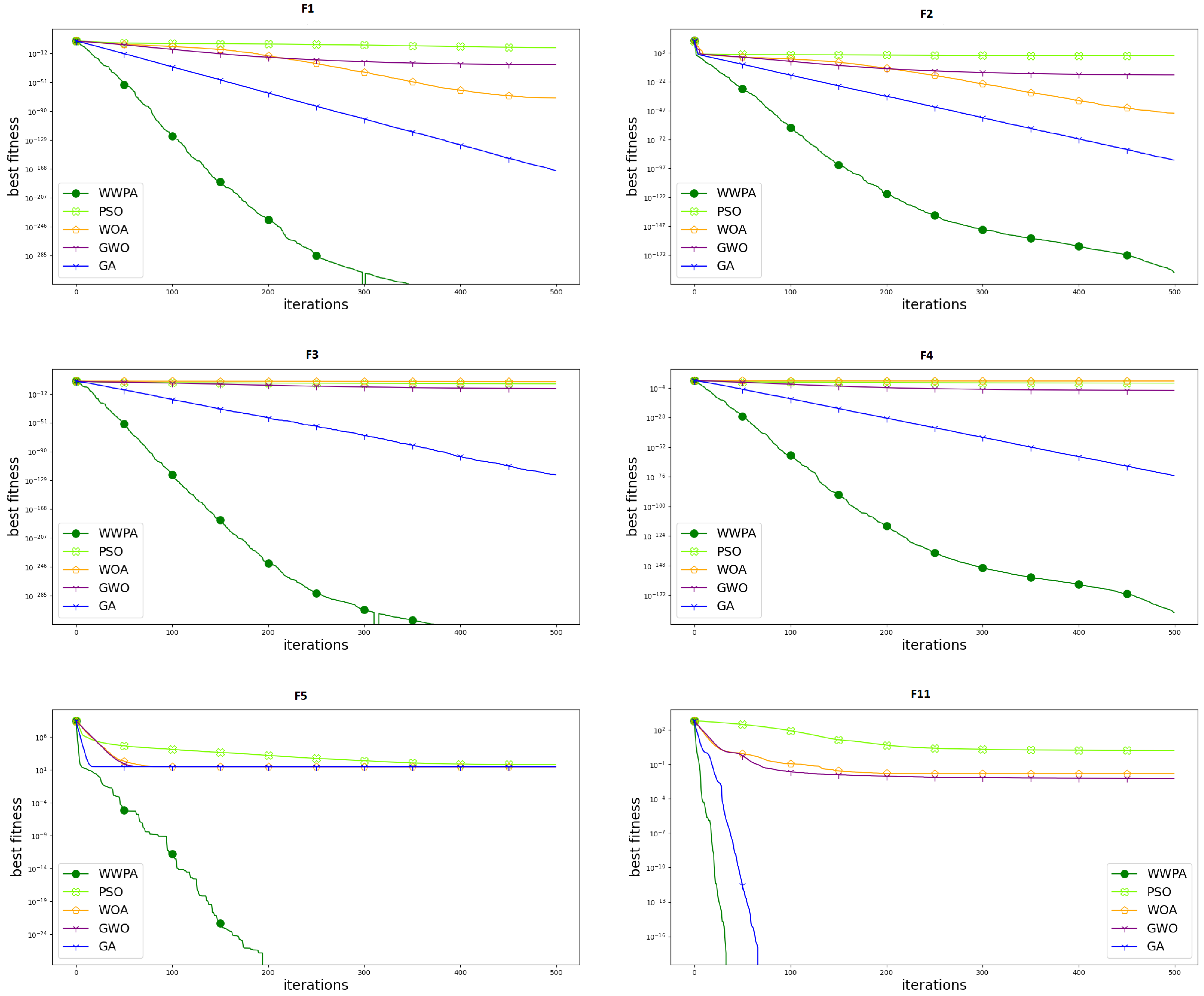
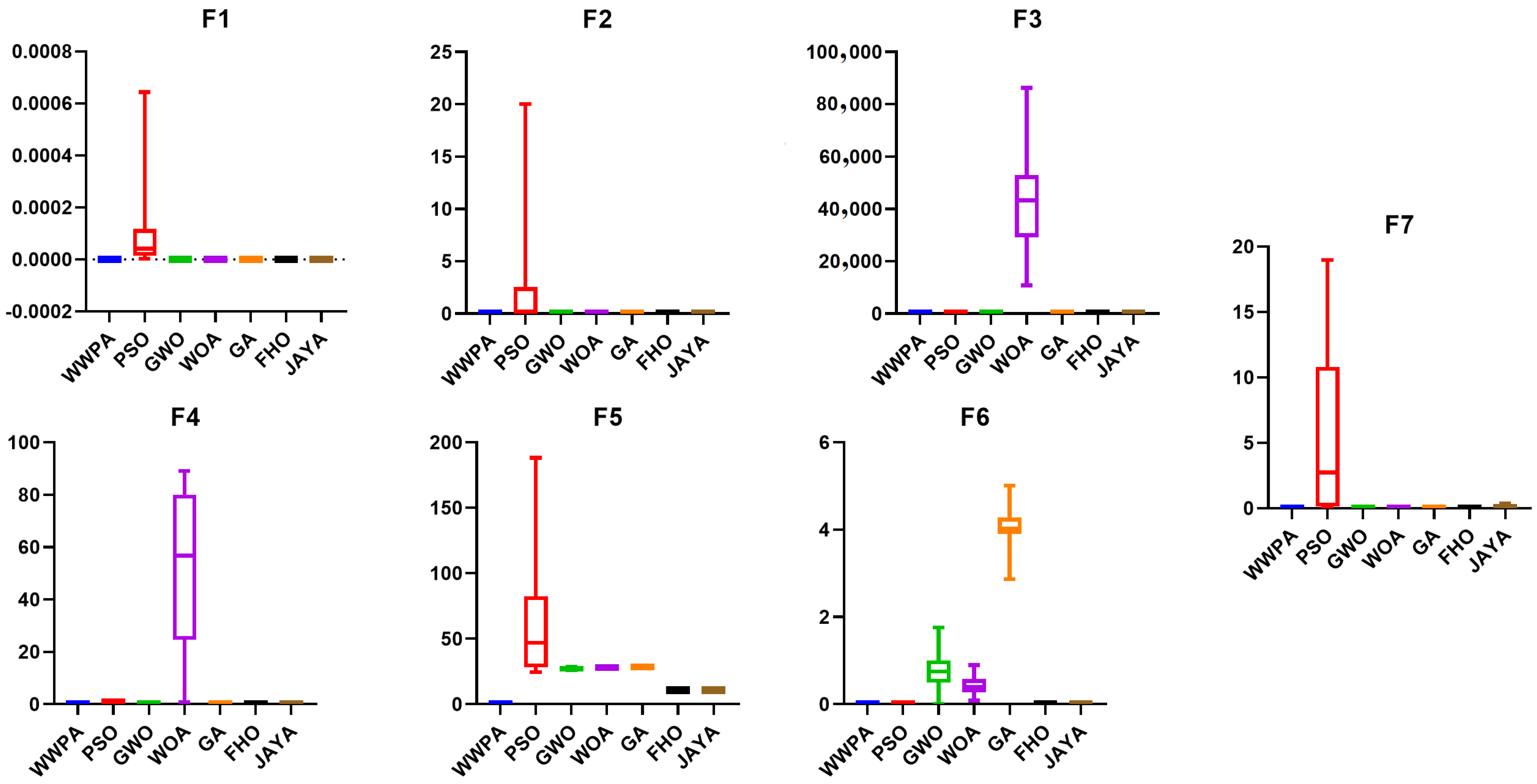
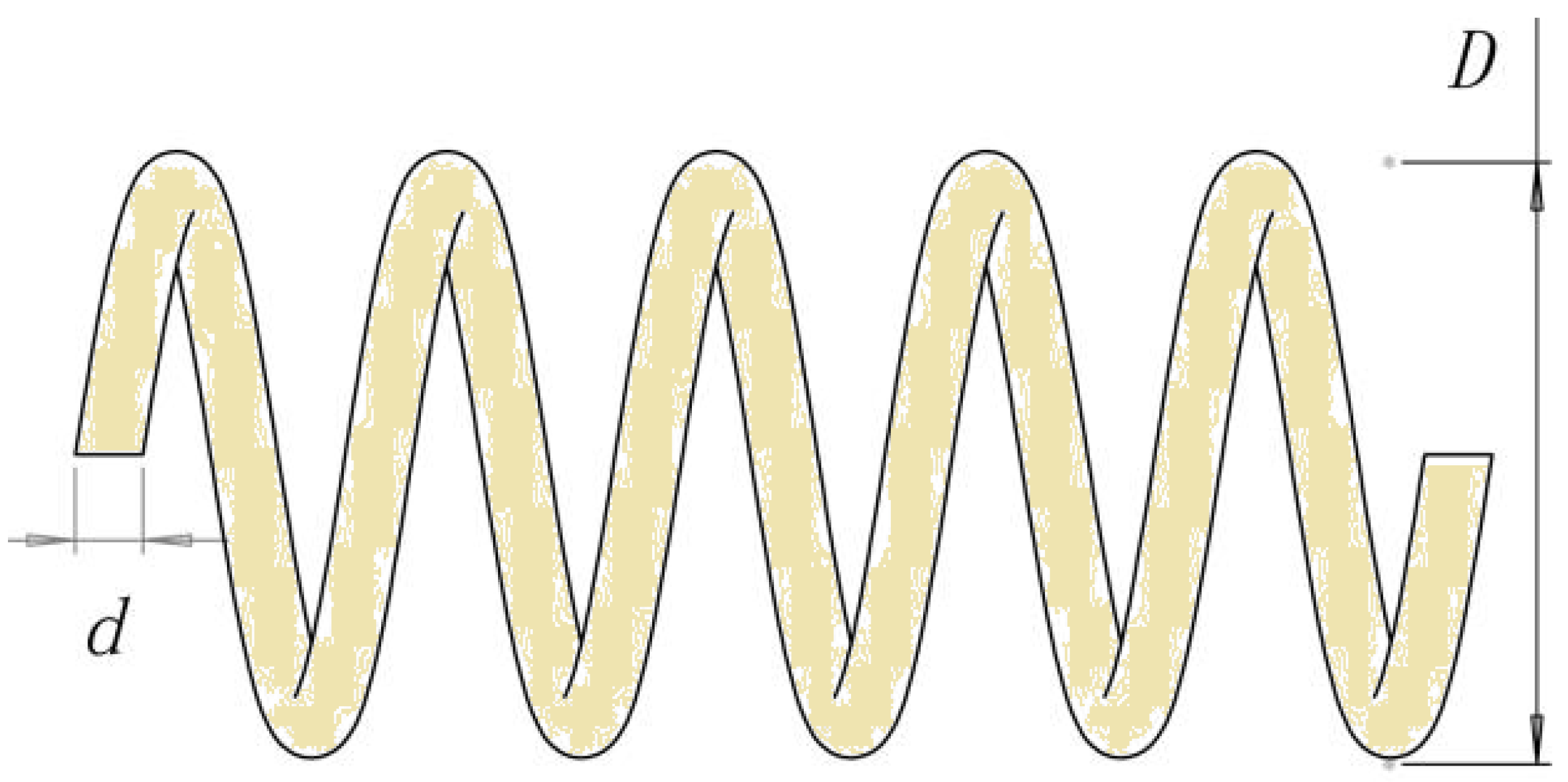
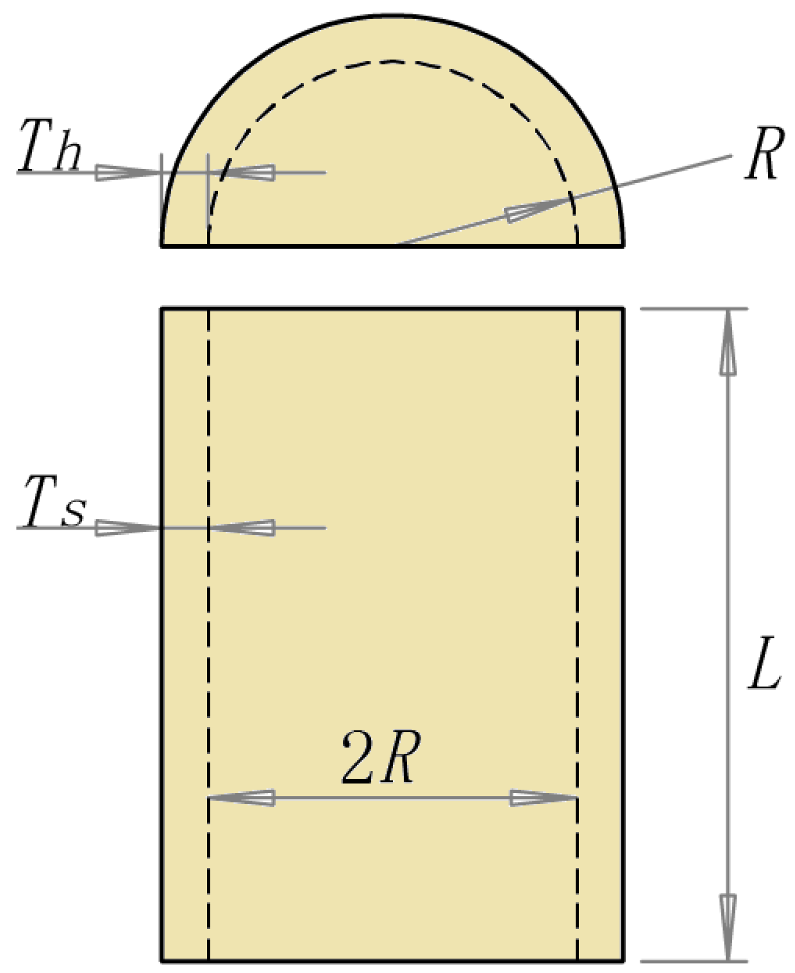
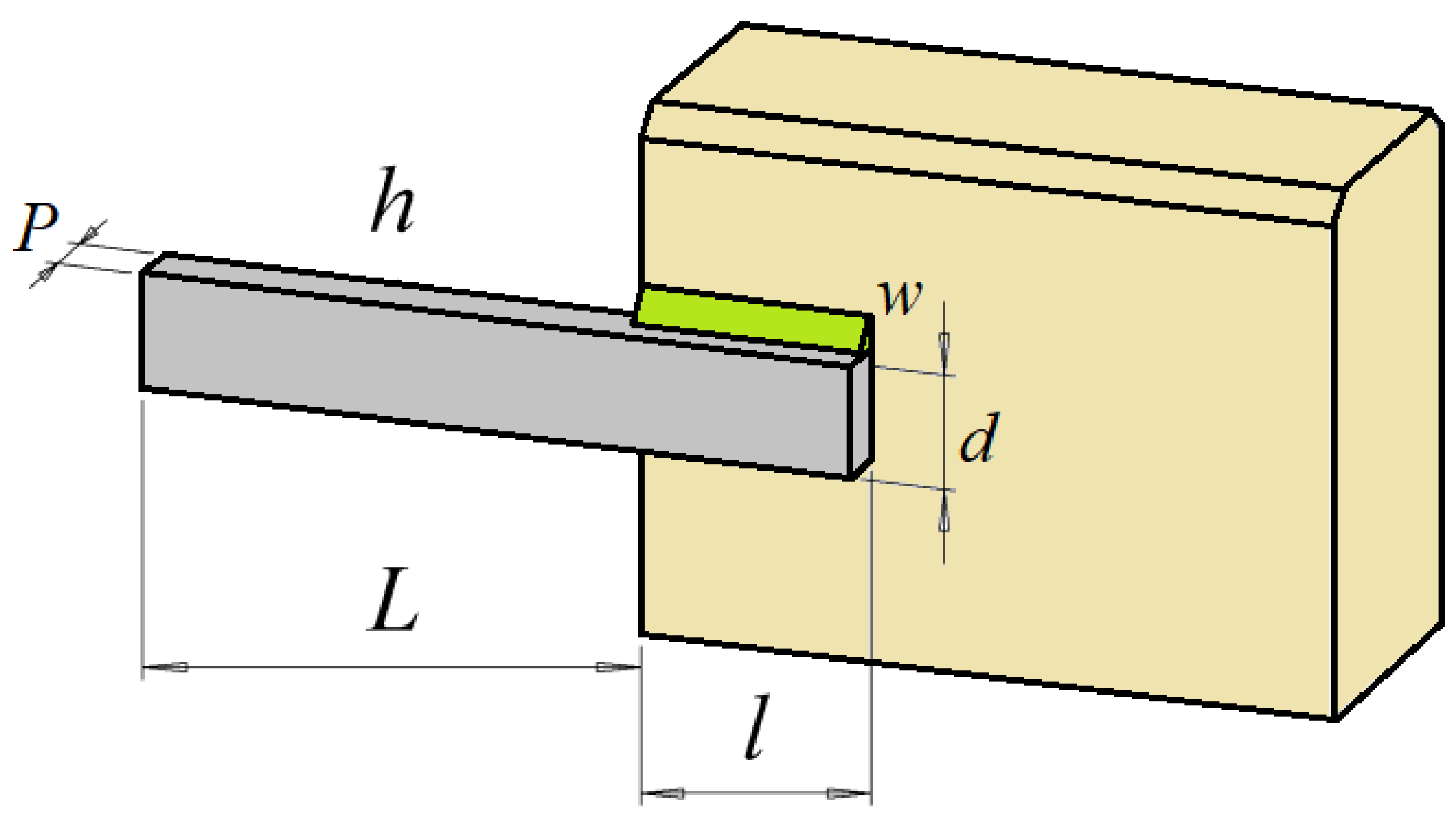
In this study, we introduce the waterwheel plant technique (WWPA), a novel swarm-based optimization technique. The planned WWPA heavily draws on the tactics and actions of waterwheel plants in the course of their search. Following an explanation of how WWPA works, a mathematical model that can be used to help with optimization issues is offered. Twenty-three objective functions from the categories of unimodal, high-dimensional multimodal, and fixed-dimensional multimodal were used to evaluate the effectiveness of the proposed method. The capabilities of the proposed algorithm were further examined by comparing the optimization results acquired by WWPA and those provided by seven other well-known algorithms: PSO, DE, WOA, GWO, GA, FHO, and JAYA. The proposed WWPA was shown to have strong exploitation power in convergently finding the global optimal solution as evidenced by the optimization results of unimodal functions. These functions’ simulation results demonstrate that WWPA outperformed eight other algorithms by a large margin when it came to fixing problems with a single modality. The multimodal function simulation results show that the proposed WWPA has strong exploration capability to test the search space and efficiently locate the ideal region. The WWPA method was superior to seven competing algorithms in simulating real-world scenarios involving multimodal optimization. The simulation results show that the proposed WWPA outperformed other methods by a wide margin in solving optimization problems. We also used WWPA to solve the difficulties of designing a pressure tank, a speed reducer, a welded beam, and a tension/compression spring. When tackling design difficulties in the real world, the simulation findings demonstrate that WWPA performed admirably.

The authors of this paper suggest several avenues for future investigation. The proposed methodology has the potential to pave the way for creating binary and multi-objective variants of WWPA, among other areas of study. In addition, the authors’ proposed directions for future research include using WWPA to address optimization problems in a wide range of scientific disciplines and real-world contexts, keeping in mind the potential of the planned WWPA for facilitating numerous future endeavors. Feature selection, data mining, COVID-19 modeling, big data, artificial intelligence, power systems, machine learning, signal denoising, wireless sensor networks, image processing, and other benchmark tasks are just some of the many areas where this approach has been put to use. It is possible that in the future, new optimizers that will perform better than WWPA in some real-world applications will be created; this is a drawback shared by all stochastic optimization approaches, including the proposed WWPA. In addition, the solutions to optimization problems obtained utilizing WWPA cannot be guaranteed to be exactly equivalent to the global optimum because of the stochastic nature of the solution approach.

References

1. Yang, X.S. Engineering Optimization: An Introduction with Metaheuristic Applications; John Wiley & Sons, Inc.: Hoboken, NJ, USA, 2010. [Google Scholar] [CrossRef]
2. Abualigah, L.; Gandomi, A.H.; Elaziz, M.A.; Hussien, A.G.; Khasawneh, A.M.; Alshinwan, M.; Houssein, E.H. Nature-Inspired Optimization Algorithms for Text Document Clustering—A Comprehensive Analysis. Algorithms 2020, 13, 345. [Google Scholar] [CrossRef]
3. Hassanien, A.E.; Emary, E. Swarm Intelligence: Principles, Advances, and Applications; CRC Press: Boca Raton, FL, USA, 2018. [Google Scholar] [CrossRef]
4. Hussien, A.G.; Hassanien, A.E.; Houssein, E.H.; Bhattacharyya, S.; Amin, M. S-shaped Binary Whale Optimization Algorithm for Feature Selection. In Recent Trends in Signal and Image Processing; Bhattacharyya, S., Mukherjee, A., Bhaumik, H., Das, S., Yoshida, K., Eds.; Advances in Intelligent Systems and Computing; Springer: Singapore, 2019; pp. 79–87. [Google Scholar] [CrossRef]
5. Fathi, H.; AlSalman, H.; Gumaei, A.; Manhrawy, I.I.M.; Hussien, A.G.; El-Kafrawy, P. An Efficient Cancer Classification Model Using Microarray and High-Dimensional Data. Comput. Intell. Neurosci. 2021, 2021, e7231126. [Google Scholar] [CrossRef]
6. Hussien, A.G.; Houssein, E.H.; Hassanien, A.E. A binary whale optimization algorithm with hyperbolic tangent fitness function for feature selection. In Proceedings of the 2017 Eighth International Conference on Intelligent Computing and Information Systems (ICICIS), Cairo, Egypt, 5–7 December 2017; pp. 166–172. [Google Scholar] [CrossRef]
7. Abdullahi, M.; Ngadi, M.A.; Dishing, S.I.; Abdulhamid, S.M.; Ahmad, B.I. An efficient symbiotic organisms search algorithm with chaotic optimization strategy for multi-objective task scheduling problems in cloud computing environment. J. Netw. Comput. Appl. 2019, 133, 60–74. [Google Scholar] [CrossRef]
8. Besnassi, M.; Neggaz, N.; Benyettou, A. Face detection based on evolutionary Haar filter. Pattern Anal. Appl. 2020, 23, 309–330. [Google Scholar] [CrossRef]
9. Neshat, M.; Mirjalili, S.; Sergiienko, N.Y.; Esmaeilzadeh, S.; Amini, E.; Heydari, A.; Garcia, D.A. Layout optimisation of offshore wave energy converters using a novel multi-swarm cooperative algorithm with backtracking strategy: A case study from coasts of Australia. Energy 2022, 239, 122463. [Google Scholar] [CrossRef]
10. Eslami, M.; Neshat, M.; Khalid, S.A. A Novel Hybrid Sine Cosine Algorithm and Pattern Search for Optimal Coordination of Power System Damping Controllers. Sustainability 2022, 14, 541. [Google Scholar] [CrossRef]
11. Nadimi-Shahraki, M.H.; Taghian, S.; Mirjalili, S.; Zamani, H.; Bahreininejad, A. GGWO: Gaze cues learning-based grey wolf optimizer and its applications for solving engineering problems. J. Comput. Sci. 2022, 61, 101636. [Google Scholar] [CrossRef]
12. Wolpert, D.; Macready, W. No free lunch theorems for optimization. IEEE Trans. Evol. Comput. 1997, 1, 67–82. [Google Scholar] [CrossRef]
13. Iba, K. Reactive power optimization by genetic algorithm. IEEE Trans. Power Syst. 1994, 9, 685–692. [Google Scholar] [CrossRef]
14. Mohar, S.S.; Goyal, S.; Kaur, R. Localization of sensor nodes in wireless sensor networks using bat optimization algorithm with enhanced exploration and exploitation characteristics. J. Supercomput. 2022, 78, 11975–12023. [Google Scholar] [CrossRef]
15. Brunetti, G.; Stumpp, C.; Šimůnek, J. Balancing exploitation and exploration: A novel hybrid global-local optimization strategy for hydrological model calibration. Environ. Model. Softw. 2022, 150, 105341. [Google Scholar] [CrossRef]
16. Xue, J.; Shen, B. A novel swarm intelligence optimization approach: Sparrow search algorithm. Syst. Sci. Control Eng. 2020, 8, 22–34. [Google Scholar] [CrossRef]
17. Mirjalili, S.; Gandomi, A.H.; Mirjalili, S.Z.; Saremi, S.; Faris, H.; Mirjalili, S.M. Salp Swarm Algorithm: A bio-inspired optimizer for engineering design problems. Adv. Eng. Softw. 2017, 114, 163–191. [Google Scholar] [CrossRef]
18. Mirjalili, S. The Ant Lion Optimizer. Adv. Eng. Softw. 2015, 83, 80–98. [Google Scholar] [CrossRef]
19. Cavazzuti, M. Optimization Methods; Springer: Berlin/Heidelberg, Germany, 2013. [Google Scholar] [CrossRef]
20. Ho, Y.C.; Pepyne, D.L. Simple Explanation of the No-Free-Lunch Theorem and Its Implications. J. Optim. Theory Appl. 2002, 115, 549–570. [Google Scholar] [CrossRef]
21. Kennedy, J.; Eberhart, R. Particle swarm optimization. In Proceedings of the ICNN’95—International Conference on Neural Networks, Perth, WA, Australia, 27 November–1 December 1995; Volume 4, pp. 1942–1948. [Google Scholar] [CrossRef]
22. Dorigo, M.; Maniezzo, V.; Colorni, A. Ant system: Optimization by a colony of cooperating agents. IEEE Trans. Syst. Man Cybern. Part B (Cybern.) 1996, 26, 29–41. [Google Scholar] [CrossRef]
23. Karaboga, D.; Basturk, B. Artificial Bee Colony (ABC) Optimization Algorithm for Solving Constrained Optimization Problems. In Proceedings of the Foundations of Fuzzy Logic and Soft Computing; Lecture Notes in Computer Science; Melin, P., Castillo, O., Aguilar, L.T., Kacprzyk, J., Pedrycz, W., Eds.; Springer: Berlin/Heidelberg, Germany, 2007; pp. 789–798. [Google Scholar] [CrossRef]
24. Osman, L. A PSPICE Fast Model for the Single Electron Transistor. Int. J. Wirel. Hoc Commun. 2021, 8–23. [Google Scholar] [CrossRef]
25. Chopra, N.; Mohsin Ansari, M. Golden jackal optimization: A novel nature-inspired optimizer for engineering applications. Expert Syst. Appl. 2022, 198, 116924. [Google Scholar] [CrossRef]
26. Dehghani, M.; Montazeri, Z.; Trojovská, E.; Trojovský, P. Coati Optimization Algorithm: A new bio-inspired metaheuristic algorithm for solving optimization problems. Knowl.-Based Syst. 2023, 259, 110011. [Google Scholar] [CrossRef]
27. Faramarzi, A.; Heidarinejad, M.; Mirjalili, S.; Gandomi, A.H. Marine Predators Algorithm: A nature-inspired metaheuristic. Expert Syst. Appl. 2020, 152, 113377. [Google Scholar] [CrossRef]
28. Abdollahzadeh, B.; Gharehchopogh, F.S.; Khodadadi, N.; Mirjalili, S. Mountain gazelle optimizer: A new nature-inspired metaheuristic algorithm for global optimization problems. Adv. Eng. Softw. 2022, 174, 103282. [Google Scholar] [CrossRef]
29. Goldberg, D.E.; Holland, J.H. Genetic Algorithms and Machine Learning. Mach. Learn. 1988, 3, 95–99. [Google Scholar] [CrossRef]
30. Castillo, O.; Ochoa, P.; Soria, J.; Castillo, O.; Ochoa, P.; Soria, J. Differential Evolution Algorithm. In Differential Evolution Algorithm with Type-2 Fuzzy Logic for Dynamic Parameter Adaptation with Application to %Intelligent Control; Springer International Publishing: Cham, Switzerland, 2021; pp. 9–12. ISBN 978-3-030-62133-9. [Google Scholar] [CrossRef]
31. Castro, L.N.d.; Timmis, J.I. Artificial immune systems as a novel soft computing paradigm. Soft Comput. 2003, 7, 526–544. [Google Scholar] [CrossRef]
32. Koza, J.R.; Koza, J.R. Genetic Programming: On the Programming of Computers by Means of Natural Selection; Google-Books-ID: Bhtxo60BV0EC; MIT Press: Cambridge, MA, USA, 1992. [Google Scholar]
33. Beyer, H.G.; Schwefel, H.P. Evolution strategies—A comprehensive introduction. Nat. Comput. 2002, 1, 3–52. [Google Scholar] [CrossRef]
34. Sebald, A.V.; Fogel, L.J. Evolutionary Programming: Proceedings of the Third Annual Conference. In Proceedings of the Evolutionary Programming, San Diego, CA, USA, 24–26 February 1994; World Scientific: Singapore, 1994; pp. 1–386. [Google Scholar] [CrossRef]
35. Shankar, K. Recent Advances in Sensing Technologies for Smart Cities. Int. J. Wirel. Hoc Commun. 2021, 1, 5–15. [Google Scholar] [CrossRef]
36. Kirkpatrick, S.; Gelatt, C.D.; Vecchi, M.P. Optimization by Simulated Annealing. Science 1983, 220, 671–680. [Google Scholar] [CrossRef] [PubMed]
37. Dehghani, M.; Montazeri, Z.; Dehghani, A.; Seifi, A. Spring search algorithm: A new meta-heuristic optimization algorithm inspired by Hooke’s law. In Proceedings of the 2017 IEEE 4th International Conference on Knowledge-Based Engineering and Innovation (KBEI), Tehran, Iran, 22 December 2017; pp. 0210–0214. [Google Scholar] [CrossRef]
38. Dehghani, M.; Samet, H. Momentum search algorithm: A new meta-heuristic optimization algorithm inspired by momentum conservation law. SN Appl. Sci. 2020, 2, 1720. [Google Scholar] [CrossRef]
39. Rashedi, E.; Nezamabadi-pour, H.; Saryazdi, S. GSA: A Gravitational Search Algorithm. Inf. Sci. 2009, 179, 2232–2248. [Google Scholar] [CrossRef]
40. Eskandar, H.; Sadollah, A.; Bahreininejad, A.; Hamdi, M. Water cycle algorithm – A novel metaheuristic optimization method for solving constrained engineering optimization problems. Comput. Struct. 2012, 110–111, 151–166. [Google Scholar] [CrossRef]
41. Mirjalili, S.; Mirjalili, S.M.; Hatamlou, A. Multi-Verse Optimizer: A nature-inspired algorithm for global optimization. Neural Comput. Appl. 2016, 27, 495–513. [Google Scholar] [CrossRef]
42. Hashim, F.A.; Hussain, K.; Houssein, E.H.; Mabrouk, M.S.; Al-Atabany, W. Archimedes optimization algorithm: A new metaheuristic algorithm for solving optimization problems. Appl. Intell. 2021, 51, 1531–1551. [Google Scholar] [CrossRef]
43. Faramarzi, A.; Heidarinejad, M.; Stephens, B.; Mirjalili, S. Equilibrium optimizer: A novel optimization algorithm. Knowl.-Based Syst. 2020, 191, 105190. [Google Scholar] [CrossRef]
44. Cuevas, E.; Oliva, D.; Zaldivar, D.; Pérez-Cisneros, M.; Sossa, H. Circle detection using electro-magnetism optimization. Inf. Sci. 2012, 182, 40–55. [Google Scholar] [CrossRef]
45. Wei, Z.; Huang, C.; Wang, X.; Han, T.; Li, Y. Nuclear Reaction Optimization: A Novel and Powerful Physics-Based Algorithm for Global Optimization. IEEE Access 2019, 7, 66084–66109. [Google Scholar] [CrossRef]
46. Pereira, J.L.J.; Francisco, M.B.; Diniz, C.A.; Antônio Oliver, G.; Cunha, S.S.; Gomes, G.F. Lichtenberg algorithm: A novel hybrid physics-based meta-heuristic for global optimization. Expert Syst. Appl. 2021, 170, 114522. [Google Scholar] [CrossRef]
47. Rao, R.V.; Savsani, V.J.; Vakharia, D.P. Teaching–learning-based optimization: A novel method for constrained mechanical design optimization problems. Comput.-Aided Des. 2011, 43, 303–315. [Google Scholar] [CrossRef]
48. Samareh Moosavi, S.H.; Bardsiri, V.K. Poor and rich optimization algorithm: A new human-based and multi populations algorithm. Eng. Appl. Artif. Intell. 2019, 86, 165–181. [Google Scholar] [CrossRef]
49. Salam, M.A. A New Method for Web Service Recommendation Based on QoS Prediction. J. Intell. Syst. Internet Things 2021, 5–14. [Google Scholar] [CrossRef]
50. Mohamed, A.W.; Hadi, A.A.; Mohamed, A.K. Gaining-sharing knowledge based algorithm for solving optimization problems: A novel nature-inspired algorithm. Int. J. Mach. Learn. Cybern. 2020, 11, 1501–1529. [Google Scholar] [CrossRef]
51. Ayyarao, T.S.L.V.; Ramakrishna, N.S.S.; Elavarasan, R.M.; Polumahanthi, N.; Rambabu, M.; Saini, G.; Khan, B.; Alatas, B. War Strategy Optimization Algorithm: A New Effective Metaheuristic Algorithm for Global Optimization. IEEE Access 2022, 10, 25073–25105. [Google Scholar] [CrossRef]
52. Dehghani, M.; Trojovský, P. Teamwork Optimization Algorithm: A New Optimization Approach for Function Minimization/Maximization. Sensors 2021, 21, 4567. [Google Scholar] [CrossRef]
53. Al-Betar, M.A.; Alyasseri, Z.A.A.; Awadallah, M.A.; Abu Doush, I. Coronavirus herd immunity optimizer (CHIO). Neural Comput. Appl. 2021, 33, 5011–5042. [Google Scholar] [CrossRef] [PubMed]
54. Dehghani, M.; Trojovská, E.; Trojovský, P. A new human-based metaheuristic algorithm for solving optimization problems on the base of simulation of driving training process. Sci. Rep. 2022, 12, 9924. [Google Scholar] [CrossRef] [PubMed]
55. Braik, M.; Ryalat, M.H.; Al-Zoubi, H. A novel meta-heuristic algorithm for solving numerical optimization problems: Ali Baba and the forty thieves. Neural Comput. Appl. 2022, 34, 409–455. [Google Scholar] [CrossRef]
56. EL-Hasnony, I.M.; Elhoseny, M.; Hassan, M.K. Intelligent Neighborhood Indexing Sequence Model for Healthcare Data Encoding. J. Intell. Syst. Internet Things 2021, 5–25. [Google Scholar] [CrossRef]
57. Moghdani, R.; Salimifard, K. Volleyball Premier League Algorithm. Appl. Soft Comput. 2018, 64, 161–185. [Google Scholar] [CrossRef]
58. Singh, P.K. Data with Turiyam Set for Fourth Dimension Quantum Information Processing. J. Neutrosophic Fuzzy Syst. 2021, 1, 9–23. [Google Scholar] [CrossRef]
59. Shiraz University of Technology; Dehghani, M.; Mardaneh, M.; Guerrero, J.; Aalborg University; Malik, O.; University of Calgary; Kumar, V.; National Institute of Technology. Football Game Based Optimization: An Application to Solve Energy Commitment Problem. Int. J. Intell. Eng. Syst. 2020, 13, 514–523. [Google Scholar] [CrossRef]
60. Arora, S.; Singh, S. Butterfly optimization algorithm: A novel approach for global optimization. Soft Comput. 2019, 23, 715–734. [Google Scholar] [CrossRef]
61. Salimi, H. Stochastic Fractal Search: A powerful metaheuristic algorithm. Knowl.-Based Syst. 2015, 75, 1–18. [Google Scholar] [CrossRef]
62. Khafaga, D.S.; Alhussan, A.A.; El-Kenawy, E.S.M.; Ibrahim, A.; Eid, M.M.; Abdelhamid, A.A. Solving Optimization Problems of Metamaterial and Double T-Shape Antennas Using Advanced Meta-Heuristics Algorithms. IEEE Access 2022, 10, 74449–74471. [Google Scholar] [CrossRef]
63. Alhussan, A.A.; Khafaga, D.S.; El-Kenawy, E.S.M.; Ibrahim, A.; Eid, M.M.; Abdelhamid, A.A. Pothole and Plain Road Classification Using Adaptive Mutation Dipper Throated Optimization and Transfer Learning for Self Driving Cars. IEEE Access 2022, 10, 84188–84211. [Google Scholar] [CrossRef]
64. Mirjalili, S.; Lewis, A. The Whale Optimization Algorithm. Adv. Eng. Softw. 2016, 95, 51–67. [Google Scholar] [CrossRef]
65. Kaveh, A.; Talatahari, S.; Khodadadi, N. Stochastic paint optimizer: Theory and application in civil engineering. Eng. Comput. 2020, 38, 1921–1952. [Google Scholar] [CrossRef]
66. Khodadadi, N.; Abualigah, L.; Mirjalili, S. Multi-objective Stochastic Paint Optimizer (MOSPO). Neural Comput. Appl. 2022, 34, 18035–18058. [Google Scholar] [CrossRef]
67. Khodadadi, N.; Mirjalili, S.M.; Mirjalili, S.Z.; Mirjalili, S. Chaotic Stochastic Paint Optimizer (CSPO). In Proceedings of the 7th International Conference on Harmony Search, Soft Computing and Applications, Seoul, Republic of Korea, 1 September 2022; pp. 195–205. [Google Scholar]
68. Heidari, A.A.; Mirjalili, S.; Faris, H.; Aljarah, I.; Mafarja, M.; Chen, H. Harris hawks optimization: Algorithm and applications. Future Gener. Comput. Syst. 2019, 97, 849–872. [Google Scholar] [CrossRef]
69. Kaveh, A.; Talatahari, S.; Khodadadi, N. The hybrid invasive weed optimization-shuffled frog-leaping algorithm applied to optimal design of frame structures. Period. Polytech. Civ. Eng. 2019, 63, 882–897. [Google Scholar] [CrossRef]
70. Chegini, S.N.; Bagheri, A.; Najafi, F. PSOSCALF: A new hybrid PSO based on Sine Cosine Algorithm and Levy flight for solving optimization problems. Appl. Soft Comput. 2018, 73, 697–726. [Google Scholar] [CrossRef]
71. El-Kenawy, E.S.M.; Mirjalili, S.; Abdelhamid, A.A.; Ibrahim, A.; Khodadadi, N.; Eid, M.M. Meta-Heuristic Optimization and Keystroke Dynamics for Authentication of Smartphone Users. Mathematics 2022, 10, 2912. [Google Scholar] [CrossRef]
72. Mirjalili, S. SCA: A Sine Cosine Algorithm for solving optimization problems. Knowl.-Based Syst. 2016, 96, 120–133. [Google Scholar] [CrossRef]
73. El-kenawy, E.S.M.; Albalawi, F.; Ward, S.A.; Ghoneim, S.S.M.; Eid, M.M.; Abdelhamid, A.A.; Bailek, N.; Ibrahim, A. Feature Selection and Classification of Transformer Faults Based on Novel Meta-Heuristic Algorithm. Mathematics 2022, 10, 3144. [Google Scholar] [CrossRef]
74. Hajiaghaei-Keshteli, M.; Aminnayeri, M. Solving the integrated scheduling of production and rail transportation problem by Keshtel algorithm. Appl. Soft Comput. 2014, 25, 184–203. [Google Scholar] [CrossRef]
75. Mosallanezhad, B.; Hajiaghaei-Keshteli, M.; Triki, C. Shrimp closed-loop supply chain network design. Soft Comput. 2021, 25, 7399–7422. [Google Scholar] [CrossRef]
76. Fathollahi-Fard, A.M.; Hajiaghaei-Keshteli, M.; Tavakkoli-Moghaddam, R. The Social Engineering Optimizer (SEO). Eng. Appl. Artif. Intell. 2018, 72, 267–293. [Google Scholar] [CrossRef]
77. Mousavi, R.; Salehi-Amiri, A.; Zahedi, A.; Hajiaghaei-Keshteli, M. Designing a supply chain network for blood decomposition by utilizing social and environmental factor. Comput. Ind. Eng. 2021, 160, 107501. [Google Scholar] [CrossRef]
78. Fathollahi-Fard, A.M.; Hajiaghaei-Keshteli, M.; Tavakkoli-Moghaddam, R. Red deer algorithm (RDA): A new nature-inspired meta-heuristic. Soft Comput. 2020, 24, 14637–14665. [Google Scholar] [CrossRef]
79. Chouhan, V.K.; Khan, S.H.; Hajiaghaei-Keshteli, M. Metaheuristic approaches to design and address multi-echelon sugarcane closed-loop supply chain network. Soft Comput. 2021, 25, 11377–11404. [Google Scholar] [CrossRef]
80. Daneshdoost, F.; Hajiaghaei-Keshteli, M.; Sahin, R.; Niroomand, S. Tabu Search Based Hybrid Meta-Heuristic Approaches for Schedule-Based Production Cost Minimization Problem for the Case of Cable Manufacturing Systems. Informatica 2022, 33, 499–522. [Google Scholar] [CrossRef]
81. Westermeier, A.S.; Sachse, R.; Poppinga, S.; Vögele, P.; Adamec, L.; Speck, T.; Bischoff, M. Supplementary material from “How the carnivorous waterwheel plant (Aldrovanda vesiculosa) snaps”. Proc. Biol. Sci. 2018, 16, 285. [Google Scholar] [CrossRef]
82. Poppinga, S.; Smaij, J.; Westermeier, A.S.; Horstmann, M.; Kruppert, S.; Tollrian, R.; Speck, T. Prey capture analyses in the carnivorous aquatic waterwheel plant (Aldrovanda vesiculosa L., Droseraceae). Sci. Rep. 2019, 9, 18590. [Google Scholar] [CrossRef]
83. Digalakis, J.; Margaritis, K. On benchmarking functions for genetic algorithms. Int. J. Comput. Math. 2001, 77, 481–506. [Google Scholar] [CrossRef]
84. Awange, J.L.; Paláncz, B.; Lewis, R.H.; Völgyesi, L. (Eds.) Particle Swarm Optimization. In Mathematical Geosciences: Hybrid Symbolic-Numeric Methods; Springer International Publishing: Cham, Switzerland, 2018; pp. 167–184. [Google Scholar] [CrossRef]
85. Immanuel, S.D.; Chakraborty, U.K. Genetic Algorithm: An Approach on Optimization. In Proceedings of the 2019 International Conference on Communication and Electronics Systems (ICCES), Coimbatore, India, 17–19 July 2019; pp. 701–708. [Google Scholar] [CrossRef]
86. Storn, R.; Price, K. Differential Evolution – A Simple and Efficient Heuristic for Global Optimization over Continuous Spaces. J. Glob. Optim. 1997, 11, 341–359. [Google Scholar] [CrossRef]
87. Rana, N.; Latiff, M.S.; Abdulhamid, S.I.; Chiroma, H. Whale optimization algorithm: A systematic review of contemporary applications, modifications and developments. Neural Comput. Appl. 2020, 32, 16245–16277. [Google Scholar] [CrossRef]
88. Mirjalili, S.; Mirjalili, S.M.; Lewis, A. Grey Wolf Optimizer. Adv. Eng. Softw. 2014, 69, 46–61. [Google Scholar] [CrossRef]
89. Venkata Rao, R. (Ed.) Jaya Optimization Algorithm and Its Variants. In Jaya: An Advanced Optimization Algorithm and its Engineering Applications; Springer International Publishing: Cham, Switzerland, 2019; pp. 9–58. [Google Scholar] [CrossRef]
90. Azizi, M.; Talatahari, S.; Gandomi, A.H. Fire Hawk Optimizer: A novel metaheuristic algorithm. Artif. Intell. Rev. 2023, 56, 287–363. [Google Scholar] [CrossRef]
91. Eid, M.M.; El-Kenawy, E.S.M.; Khodadadi, N.; Mirjalili, S.; Khodadadi, E.; Abotaleb, M.; Alharbi, A.H.; Abdelhamid, A.A.; Ibrahim, A.; Amer, G.M.; et al. Meta-Heuristic Optimization of LSTM-Based Deep Network for Boosting the Prediction of Monkeypox Cases. Mathematics 2022, 10, 3845. [Google Scholar] [CrossRef]
92. Samee, N.A.; El-Kenawy, E.S.M.; Atteia, G.; Jamjoom, M.M.; Ibrahim, A.; Abdelhamid, A.A.; El-Attar, N.E.; Gaber, T.; Slowik, A.; Shams, M.Y. Metaheuristic Optimization through Deep Learning Classification of COVID-19 in Chest X-ray Images. Comput. Mater. Contin. 2022, 73, 4193–4210. [Google Scholar] [CrossRef]
93. Celik, Y.; Kutucu, H. Solving the Tension/Compression Spring Design Problem by an Improved Firefly Algorithm. In Proceedings of the IDDM, Lviv, Ukraine, 28–30 November 2018. [Google Scholar]
94. Zou, D.; Liu, H.; Gao, L.; Li, S. A novel modified differential evolution algorithm for constrained optimization problems. Comput. Math. Appl. 2011, 61, 1608–1623. [Google Scholar] [CrossRef]
95. Ragsdell, K.M.; Phillips, D.T. Optimal Design of a Class of Welded Structures Using Geometric Programming. J. Eng. Ind. 1976, 98, 1021–1025. [Google Scholar] [CrossRef]
96. Khafaga, D.S.; Alhussan, A.A.; El-kenawy, E.M.; Ibrahim, A.; Elkhalik, S.H.A.; El-Mashad, S.Y.; Abdelhamid, A.A. Improved Prediction of Metamaterial Antenna Bandwidth Using Adaptive Optimization of LSTM. Comput. Mater. Contin. 2022, 73, 865–881. [Google Scholar] [CrossRef]
Figure 1. Image of the waterwheel plant [81]. (a) Lateral view of a free-floating shoot with numerous traps. (b) Frontal view with open and closed traps. (c) Single open trap. (d) Schematic drawing of an open trap.
Processes 11 01502 g001
Figure 2. The inspiration of the proposed methodology.
Processes 11 01502 g002
Figure 3. Three-dimensional images of typical functions: F 1 , F 2 , F 3 , F 4 , F 5 , and F 7 .
Processes 11 01502 g003
Figure 4. Convergence curves of the presented and compared algorithms for functions f 1 , f 2 , f 3 , f 4 , f 5 , and f 11 .
Processes 11 01502 g004
Figure 5. Visualization of the analysis of the results of solving the benchmark functions.
Processes 11 01502 g005
Figure 6. Inspiration of the proposed methodology.
Processes 11 01502 g006
Figure 7. Tension/compression spring design problem.
Processes 11 01502 g007
Figure 8. Pressure vessel design problem.
Processes 11 01502 g008
Figure 9. Welded beam design problem.
Processes 11 01502 g009