Bifurcation Analysis for an OSN Model with Two Delays

Abstract

In this research, we introduce and analyze a mathematical model for online social networks, incorporating two distinct delays. These delays represent the time it takes for active users within the network to begin disengaging, either with or without contacting non-users of online social platforms. We focus particularly on the user prevailing equilibrium (UPE), denoted as $P^{*}$, and explore the role of delays as parameters in triggering Hopf bifurcations. In doing so, we find the conditions under which Hopf bifurcations occur, then establish stable regions based on the two delays. Furthermore, we delineate the boundaries of stability regions wherein bifurcations transpire as the delays cross these thresholds. We present numerical simulations to illustrate and validate our theoretical findings. Through this interdisciplinary approach, we aim to deepen our understanding of the dynamics inherent in online social networks.

1. Introduction

The emergence of online social networks (OSNs) has significantly reshaped the landscape of information dissemination and interpersonal connectivity over the last two decades. Platforms like Facebook, Twitter, and Instagram have revolutionized how individuals exchange ideas and interact, profoundly influencing daily life. OSNs serve as virtual spaces where users can present themselves, engage with others, and forge connections irrespective of geographical boundaries. Their widespread adoption, particularly among tech-savvy generations, has had far-reaching implications across various domains, such as education, elections, and information dissemination. Understanding the intricate ways in which OSNs influence societal, political, and economic realms, as well as individual behaviors, has become increasingly imperative.

To better comprehend the dynamics of OSNs, mathematical models have been developed, offering profound insights into how social networks shape opinions and behaviors. Noteworthy contributions include seminal works by, for example [1,2,3,4,5,6,7,8,9,10,11]. Many of these models draw inspiration from SIR/SEIR disease-type models, providing a framework to study OSN dynamics effectively. Interested readers can delve into classic and advanced results on SIR/SEIR mathematical models and SIR/SEIR mathematical models with delays in works such as those by [12,13,14,15,16,17,18,19,20,21,22,23,24] and references therein. Most recently, Barman and Mishra [25,26] introduced a graph Laplacian diffusion into SIR/SEIR type network models and carried out Hopf bifurcation analysis.

In the realm of OSN modeling, the total population $N\left(t\right)$ at time t is often partitioned into three distinct sub-classes representing key populations within OSN dynamics: potential users, active users, and individuals opposed to OSNs, denoted by $x\left(t\right)$, $y\left(t\right)$, and $z\left(t\right)$, respectively. Cannarella and Spechler [2] introduced the “infectious recovery” SIR-type model to analyze user adoption and abandonment of OSNs, later extended in ordinary, fractional, and stochastic differential equation models as given in [3,5,6]. Graef et al. [5] explored the following OSN model with demography to examine adoption and abandonment dynamics, conducting both local and global stability analyses.

$$\left\{\begin{array}{c}{x}^{\prime }=\Lambda -\alpha xy-\mu x,\hfill \\ y^{\prime }=\alpha xy-\eta yz-(\mu +\delta )y,\hfill \\ z^{\prime }=\eta yz+\delta y-\mu z.\hfill \end{array}\right.$$

(1)

Motivated by existing research and the nuanced complexities of OSNs, Wang and Wang [27] proposed a dynamic mathematical model capturing unique characteristics such as users’ varying interests and the impact of time delays. Their model accounts for the transition of potential users to active ones and the eventual abandonment of OSNs by active users due to disinterest or interaction with those opposed to OSNs. This interaction is described by a system of differential equations as follows:

$$\begin{array}{c}\hfill \left\{\begin{array}{ccc}\hfill x^{\prime }& =& A-\alpha xy-\mu x,\hfill \\ \hfill y^{\prime }& =& \alpha xy-\eta y\left(t\right)z\left(t\right)-\delta y(t-\tau )-\mu y,\hfill \\ \hfill z^{\prime }& =& B+\eta y\left(t\right)z\left(t\right)+\delta y(t-\tau )-\mu z,\hfill \end{array}\right.\end{array}$$

(2)

where the parameters $A>0$ and $B\ge 0$ represent the rates that newcomers come into the community as either potential online network users or as people who are never interested in OSNs. $\alpha >0$ denotes the contact rate between the potential and active OSN users; $\mu >0$ is the death rate for all people; $\eta >0$ is the contact rate between active users and people who are opposed to OSNs; $\delta >0$ is the transferring rate describing the rate the active users lose their interest and become opposing to OSNs; and $\tau \ge 0$ is the time delay that represents the time for active users to starting abandoning the network. Wang and Wang [27] performed a detailed analysis for System (2), including local and global analysis for user free equilibrium (UFE) and UPE. Hopf bifurcation was also carried out using the delay $\tau$ as the bifurcating parameter. Conditions and critical values were found that guarantee the occurrence of Hopf bifurcation.

Building upon prior work, considering the fact that it will take some time for active users to disengage after interacting with non-users, we introduce the following refined model that accounts for this time delay. Our proposed system of equations incorporates a time delay $\rho$, representing the period for active users to abandon OSNs after contact with non-users. This addition of a new time delay can indeed make it more representative of real-world situations and more accurately representing real-world dynamics and improving the reliability of predictions and control strategies. Notably, our model encompasses previous formulations as special cases, offering a comprehensive framework to study the evolving dynamics of OSNs

$$\begin{array}{c}\hfill \left\{\begin{array}{ccc}\hfill x^{\prime }& =& A-\alpha xy-\mu x,\hfill \\ \hfill y^{\prime }& =& \alpha xy-\eta y(t-\rho )z(t-\rho )-\delta y(t-\tau )-\mu y,\hfill \\ \hfill z^{\prime }& =& B+\eta y(t-\rho )z(t-\rho )+\delta y(t-\tau )-\mu z.\hfill \end{array}\right.\end{array}$$

(3)

For System (3), define

$$\begin{array}{c}\hfill f\left(z\right)=A\alpha (\delta +\eta z)\end{array}$$

(4)

and

$$\begin{array}{c}\hfill g\left(z\right)=\mu \eta (\alpha +\eta )z^2+[\mu (\mu +\delta )(\alpha +\eta )+\eta (\mu \delta -B\alpha )]z+(\mu +\delta )(\mu \delta -B\alpha ).\end{array}$$

(5)

Let $R_0$ be the basic reproduction number defined by

$$R_0=\frac{A\alpha }{B\eta +\mu (\mu +\delta )}.$$

(6)

The following results are established by Wang and Wang [27].

Theorem 1.

Let $R_0$ be defined by (6). If $R_0\le 1,$ then System (3) has a unique user free equilibrium $P_0=(A/\mu ,0,B/\mu )$ and it exists for all parameter values. If $R_0>1,$ then System (3) has two equilibria: $P_0$ and a unique user prevailing equilibrium $P^{*}=(x^{*},y^{*},z^{*}),$ where $z^{*}$ is the unique positive root of the equation $f\left(z\right)=g\left(z\right)$, such that $z^{*}>B/\mu ,$ and $x^{*}$ and $y^{*}$ are given by

$$x^{*}=\frac{\mu +\delta }{\alpha }+\frac{\eta }{\alpha }{z}^{*},$$

(7)

and

$$y^{*}=\frac{\mu z^{*}-B}{\delta +\eta z^{*}}.$$

(8)

Theorem 2.

Let $R_0$ be defined by (6) and assume that $\tau =\rho =0$. If $R_0<1,$ $P_0$ is locally asymptotically stable; if $R_0=1,$ $P_0$ is neutrally stable; and if $R_0>1,$ $P_0$ becomes unstable, and $P^{*}$ emerges and it is locally asymptotically stable.

The following result was established by Ruan and Wei [28] and will be used in this research.

Lemma 1.

Consider the following exponential polynomial:

$$\begin{array}{ccc}P(\lambda ,{\tau }_1,{\tau }_2,\cdots ,{\tau }_m)\hfill & =\hfill & {\lambda }^n+a_1^{\left(0\right)}{\lambda }^{n-1}+\cdots +a_n^{\left(0\right)}\hfill \\ \hfill & +\hfill & [a_1^{\left(1\right)}{\lambda }^{n-1}+\cdots +a_n^{\left(1\right)}]e^{-\lambda {\tau }_1}\hfill \\ \hfill & +\hfill & \cdots \hfill \\ \hfill & +\hfill & [a_1^{\left(m\right)}{\lambda }^{n-1}+\cdots +a_n^{\left(m\right)}]e^{-\lambda {\tau }_m},\hfill \end{array}$$

where ${\tau }_i\ge 0(i=1,2,\cdots ,m)$ and $a_j^{\left(i\right)}(i=0,1,2,\cdots ,m;j=1,2,\cdots ,n)$ are constants. As $({\tau }_1,{\tau }_2,\cdots ,{\tau }_m)$ changes, the sum of the orders of the zeros of P in the open right half plane can change only if a zero appears on or crosses the imaginary axis.

In this research, we were interested in finding out what network user dynamics the new model presents, in particular, whether or not a Hopf bifurcation will occur for this new OSN model after adding a time delay. In doing so, we performed a Hopf bifurcation analysis for System (3) using two delays $\tau$ and $\rho$ as bifurcating parameters. We investigated the Hopf bifurcations at the unique user prevailing equilibrium point when $R_0>1$. Stability regions were established in terms of two delays $\tau$ and $\rho .$ Conditions and critical curves were obtained so that the Hopf bifurcation occurs as $(\tau ,\rho )$, passing through the boundary of the stability regions.

The remainder of the manuscript is structured as follows: In Section 2, we delve into Hopf bifurcation analysis concerning the interplay of two delays. We explore the establishment of stability regions and identify critical values under scenarios where either one delay is absent, or both delays are concurrently present. Our investigation delves into the conditions conducive to Hopf bifurcations and delineates the associated implications. To augment our theoretical insights, we present numerical simulations aimed at illustrating the dynamics of the system under consideration.

Finally, Section 3 encapsulates our findings and conclusions drawn from the preceding analyses. We synthesize the key insights gleaned from our study and discuss their broader implications in understanding the dynamics of online social networks.

2. Hopf Bifurcation

From Wang and Wang [27], we know that the dynamics of System (3) is completely determined by the basic reproduction number $R_0$ when delays $\rho =\tau =0.$ In particular, we know that when $R_0>1,$ the unique user prevailing equilibrium $P^{*}$ is locally asymptotically stable. We are interested in the question of whether the delays $\rho$ and $\tau$ could cause the stability of the UPE $P^{*}$ to switch as they increase. In this section, we study the occurrence of Hopf bifurcations using the delays $\rho$ and $\tau$ as the bifurcation parameters. Note that when $R_0>1$ there is a unique UPE $P^{*}=(x^{*},y^{*},z^{*}).$ For this section, we always assume that $R_0>1.$

The characteristic equation of System (3) at the unique equilibrium $P^{*}$ when $\rho ,\tau \ge 0$ is the determinant of the matrix

$$J^{*}=\left(\begin{array}{ccc}\lambda +\alpha y^{*}+\mu & \alpha x^{*}& 0\\ -\alpha y^{*}& \lambda +\mu -\alpha x^{*}+\eta z^{*}{e}^{-\lambda \rho }+\delta e^{-\lambda \tau }& \eta y^{*}{e}^{-\lambda \rho }\\ 0& -\eta z^{*}{e}^{-\lambda \rho }-\delta e^{-\lambda \tau }& \lambda +\mu -\eta y^{*}{e}^{-\lambda \rho }\end{array}\right),$$

which is

$$(\lambda +\mu )({\lambda }^2+a\lambda +b+\eta (c\lambda +d)e^{-\lambda \rho }+\delta (\lambda +h)e^{-\lambda \tau })=0,$$

(9)

where

$$\begin{array}{ccc}\hfill a& =& 2\mu +\alpha y^{*}-\alpha x^{*},\hfill \\ \hfill b& =& \mu (\mu +\alpha y^{*}-\alpha x^{*}),\hfill \\ \hfill c& =& z^{*}-y^{*},\hfill \\ \hfill d& =& (z^{*}-y^{*})(\mu +\alpha y^{*})+\alpha x^{*}{y}^{*},\hfill \\ \hfill h& =& \mu +\alpha y^{*},\hfill \end{array}$$

(10)

and $x^{*},y^{*}$, and $z^{*}$ are given in Theorem 1.

One root of Equation (9) is $\lambda =-\mu <0.$ The other roots are determined by the transcendental equation:

$${\lambda }^2+a\lambda +b+\eta (c\lambda +d)e^{-\lambda \rho }+\delta (\lambda +h)e^{-\lambda \tau }=0.$$

(11)

We know that if $R_0>1$ and $\rho =\tau =0,$ all roots of Equation (11) have negative real parts and $P^{*}$ is locally asymptotically stable. Our interest is to see whether or not the delays $\rho$ and $\tau$ cause the stability of $P^{*}$ to switch as $\rho$ and $\tau$ increase while $R_0$ remains larger than the unity. Due to Lemma 1, we need to investigate if a zero of Equation (11) appears on or crosses the imaginary axis as $\rho$ and $\tau$ increases. Keep in mind that when $R_0>1,$ $z^{*}>B/\mu ,$ see [27].

From (10) and using the expressions given in (7) and (8), we can obtain

$$b+\eta d+\delta h=\frac{(\mu z^{*}-B)\left(\alpha \left(\eta \left(B+\eta {\left(z^{*}\right)}^2\right)+{\delta }^2+\delta (\mu +2\eta z^{*})\right)+\eta {(\delta +\eta z^{*})}^2\right)}{{(\delta +\eta z^{*})}^2}>0$$

since $z^{*}>B/\mu .$ Therefore, $\lambda =0$ is not a root of (11). Therefore, there are no zero-Hopf bifurcations.

2.1. Hopf Bifurcation When $\rho =0$

For the case that $\rho =0,$ the Hopf bifurcation analysis was carried out completely by Wang and Wang [27]. For completeness, we only cite key definitions and results here. We refer readers to [27] for a detailed analysis. When $\rho =0,$ Equation (11) becomes

$${\lambda }^2+a_1\lambda +b_1+(\delta \lambda +c_1)e^{-\lambda \tau }=0,$$

(12)

where

$$\begin{array}{ccc}\hfill a_1& =& 2\mu +\alpha y^{*}+\eta z^{*}-\alpha x^{*}-\eta y^{*},\hfill \\ \hfill b_1& =& {\mu }^2+\mu (\alpha y^{*}+\eta z^{*}-\alpha x^{*}-\eta y^{*})+\alpha \eta y^{*}(x^{*}+z^{*}-y^{*}),\hfill \\ \hfill c_1& =& \delta (\mu +\alpha y^{*}).\hfill \end{array}$$

(13)

Now, let $\lambda =\omega i$ ($\omega >0$) be a root to Equation (12). Plug it into (12), then $\omega$ has to satisfy the following equation:

$${\omega }^4+(a_1^2-{\delta }^2-2b_1){\omega }^2+b_1^2-c_1^2=0.$$

Let $p=w^2$ and denote $a_2=a_1^2-{\delta }^2-2b_1$ and $b_2=b_1^2-c_1^2.$ Then, the above equation can be rewritten as:

$$p^2+a_{2}p+b_2=0.$$

(14)

The following result is well known.

Lemma 2.

For Equation (14), we have

(a)

If $b_2<0$ or if $b_2=0$ and $a_2<0,$ then it has a unique positive root.

(b)

If $a_2\ge 0$ and $b_2\ge 0,$ then it has no positive roots.

(c)

If $a_2<0$ and $b_2>0,$ then it has no positive roots if $a_2^2-4b_2<0;$ one positive root if $a_2^2-4b_2=0;$ and two positive roots if $a_2^2-4b_2>0.$

Plug $a_1,b_1,c_1$, given in (13) and $x^{*}$, and $y^{*}$, given in (7) and (8), into $a_2$ and $b_2,$ and we have

$$\begin{array}{cc}\hfill a_2=& a_1^2-{\delta }^2-2b_1=\frac{1}{{(\delta +\eta z^{*})}^2}{P}_1\left(z^{*}\right),\hfill \end{array}$$

(15)

$$\begin{array}{cc}\hfill b_2=& b_1^2-c_1^2=\frac{(\mu z^{*}-B)}{{(\delta +\eta z^{*})}^4}{P}_2\left(z^{*}\right)P_3\left(z^{*}\right),\hfill \end{array}$$

(16)

where

$$\begin{array}{ccc}\hfill P_1\left(z\right)& =& -2{\eta }^2\mu (\alpha +\eta )z^3+(2B{\eta }^2(\alpha +\eta )+\mu ({\alpha }^2\mu -4\alpha \delta \eta -2\alpha \delta {\eta }^2))z^2\hfill \\ & & +(B(4\alpha \delta \eta +2\delta {\eta }^2-2\alpha \mu )-2\alpha {\delta }^2\mu )z\hfill \\ & & +B^2({\eta }^2+{\alpha }^2)+{\delta }^2{\mu }^2+2B\delta (\alpha \delta +\eta \mu ),\hfill \end{array}$$

(17)

$$\begin{array}{ccc}\hfill P_2\left(z\right)& =& (\alpha {\eta }^2+{\eta }^3)z^2+(2\alpha \delta \eta +2\delta {\eta }^2)z+\alpha {\delta }^2+\alpha \delta \mu +\alpha B\eta +{\delta }^2\eta ,\hfill \\ \hfill P_3\left(z\right)& =& (\alpha {\eta }^2\mu +{\eta }^3\mu )z^3-(\alpha B{\eta }^2+B{\eta }^3)z^2\hfill \\ & & +(-\alpha {\delta }^2\mu +\alpha \delta {\mu }^2+\alpha B\eta \mu -2B\delta {\eta }^2-3{\delta }^2\eta \mu )z\hfill \\ & & -\alpha B^2\eta +\alpha B{\delta }^2-\alpha B\delta \mu -B{\delta }^2\eta -2{\delta }^3\mu .\hfill \end{array}$$

(18)

We then have the following results; see Wang and Wang [27].

Theorem 3.

Let $R_0>1,$ and let $a_2,b_2,P_1$ and $P_3$ be defined by (15), (16), (17), and (18). Assume that $P_1$ and $P_3$ have unique positive roots $z_1$ and $z_2,$ respectively.

(I)

When any of the following conditions is satisfied, Equation (14) has no positive roots.

(1)

$z_1=z_2$ and $z^{*}=z_1;$

(2)

$z_1>z_2$ and $z_2\le z^{*}\le z_1;$

(3)

$z^{*}>max\{z_1,z_2\}$ and $a_2^2-4b_2<0.$

(II)

When any of the following conditions is satisfied, Equation (14) has a unique positive root.

(1)

$z_1<z_2$ and $z^{*}\le z_2;$

(2)

$z_1\ge z_2$ and $z^{*}<z_2;$

(3)

$z^{*}>max\{z_1,z_2\}$ and $a_2^2-4b_2=0.$

(III)

Equation (14) has two positive roots if $z^{*}>max\{z_1,z_2\}$ and $a_2^2-4b_2>0$.

Now assume that $R_0>1$ and Equation (14) has at least one positive root. Solving p from Equation (14) for the positive roots gives

$$p^{\pm }=\frac{1}{2}\left[-(a_1^2-{\delta }^2-2b_1)\pm \sqrt{{(a_1-{\delta }^2-2b_1)}^2-4(b_1^2-c_1^2)}\right].$$

Note that if Equation (14) has a unique positive root, then it is $p^{+}.$ Let ${\omega }^{\pm }=\sqrt{p^{\pm }}$ and define

$$f_1\left(\omega \right)=\frac{c_1{\omega }^2-a_1\delta {\omega }^2-b_1{c}_1}{c_1^2+{\delta }^2{\omega }^2}$$

and

$$f_2\left(\omega \right)=\frac{\omega (a_1{c}_1-b_1\delta +\delta {\omega }^2)}{c_1^2+{\delta }^2{\omega }^2}.$$

Also define ${\tau }_n^{\pm },n=0,1,2,\cdots ,$ as

$${\tau }_n^{\pm }=\left\{\begin{array}{cc}\frac{1}{{\omega }^{\pm }}(arccos{f}_1\left({\omega }^{\pm }\right)+2n\pi )\hfill & \mathrm{if}{f}_2\left({\omega }^{\pm }\right)>0,\hfill \\ \frac{1}{{\omega }^{\pm }}(2\pi -arccos{f}_1\left({\omega }^{\pm }\right)+2n\pi )\hfill & \mathrm{if}{f}_2\left({\omega }^{\pm }\right)\le 0.\hfill \end{array}\right.$$

(19)

Hence, ${\tau }_n^{\pm }>0$ and Equation (11) has a pair of purely imaginary roots $\pm i{\omega }^{\pm }$ when $\tau ={\tau }_n^{\pm }$ for $n=0,1,2,\cdots .$

Theorem 4.

Assume that $R_0>1$ and let $a_2,b_2,P_1,P_3,z^{*},{\omega }^{+},{\tau }_0^{+}$ be defined above. Assume that $P_1$ and $P_3$ have unique positive roots $z_1$ and $z_2,$ respectively. We then have the following results.

(I)

All roots of Equation (12) have negative real parts for all delay $\tau \ge 0,$ if

(1)

$z_1=z_2$ and $z^{*}=z_1,$ or

(2)

$z_1>z_2$ and $z_2\le z^{*}\le z_1,$ or

(3)

$z^{*}>max\{z_1,z_2\}$ and $a_2^2-4b_2<0.$

Therefore, $P^{*}$ is locally asymptotically stable for all $\tau \ge 0.$

(II)

There is a ${\tau }_0^{+}>0$, such that all roots of Equation (12) have negative real parts for all $\tau \in [0,{\tau }_0^{+})$. It has a pair of purely imaginary roots $\pm i{\omega }^{+}$, and all other roots have negative real parts when $\tau ={\tau }_0^{+},$ if

(1)

$z_1<z_2$ and $z^{*}\le z_2,$ or

(2)

$z_1\ge z_2$ and $z^{*}<z_2,$ or

(3)

$z^{*}>max\{z_1,z_2\}$ and $a_2^2-4b_2\ge 0.$

Therefore, $P^{*}$ is locally asymptotically stable for all $\tau <{\tau }_0^{+}.$ Hopf bifurcation occurs as τ passes through $\tau ={\tau }_0^{+}$.

We use one numerical simulation to illustrate the above theoretical results. If we choose $A=10,B=0.2,\alpha =0.1,\eta =0.5,\mu =0.2,\delta =0.4.$ Then we have $P^{*}=(43.239,0.3127,7.4479),$ i.e., $z^{*}=7.4479.$ Calculations show that $R_0=4.54545>1,$ and

$$a_1=0.325082,b_1=0.682603,c_1=0.092508.$$

Two polynomials $P_1$ and $P_3$ can be found:

$$\begin{array}{ccc}\hfill P_1\left(z\right)& =& 0.0392+0.0488z+0.0044z^2-0.06z^3,\hfill \\ \hfill P_3\left(z\right)& =& -0.042-0.0876z-0.03z^2+0.03z^3.\hfill \end{array}$$

By Descartes’ Rule of Signs, both $P_1$ and $P_3$ have a unique positive root and they are

$$z_1=1.20208,z_2=2.43518.$$

We also find that

$$a_2=-1.41953,b_2=0.457389.$$

Thus

$$a_2^2-4b_2=0.185503>0.$$

Therefore, Condition (II)(3) of Theorem 4 is satisfied and a ${\tau }_0^{+}>0$ exists. Using (19), we find that

$${\tau }_0^{+}=0.440535.$$

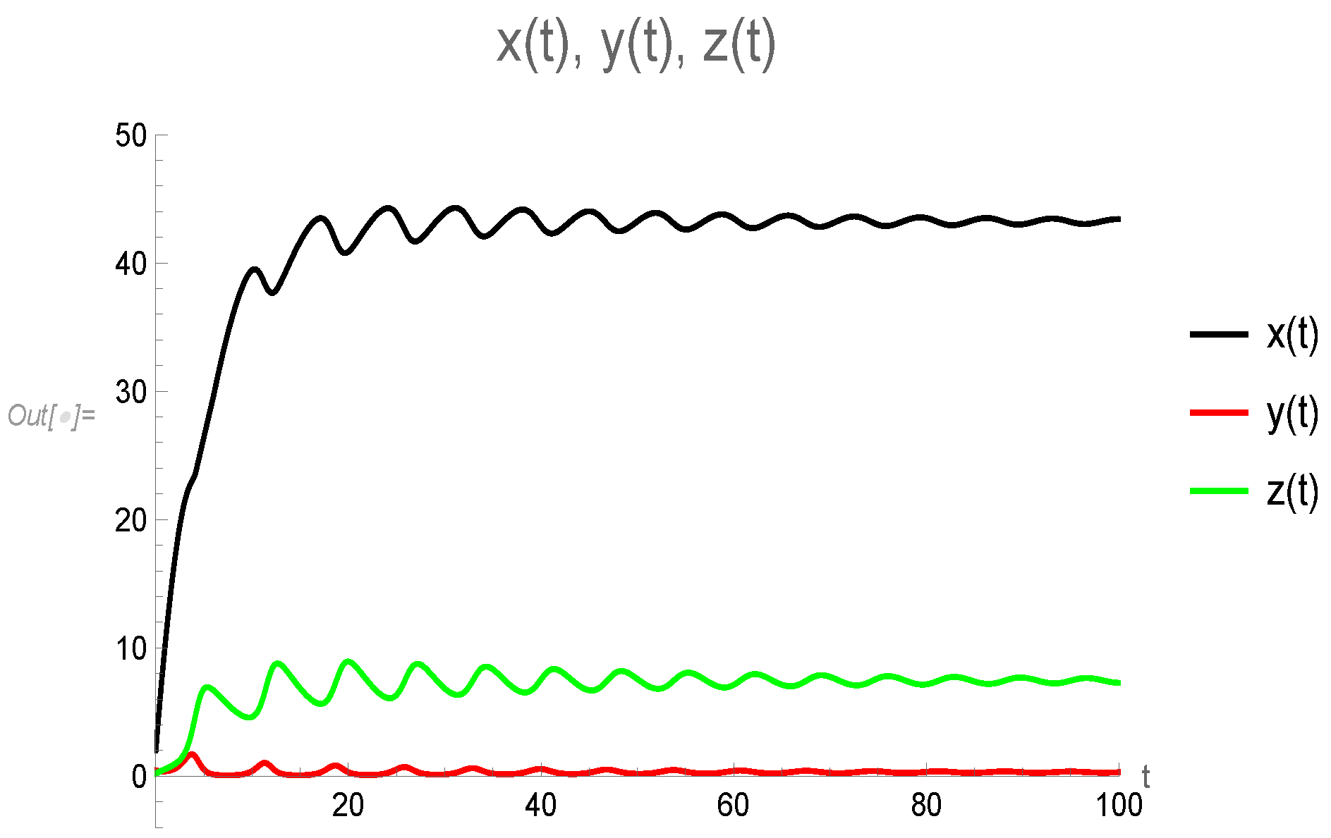
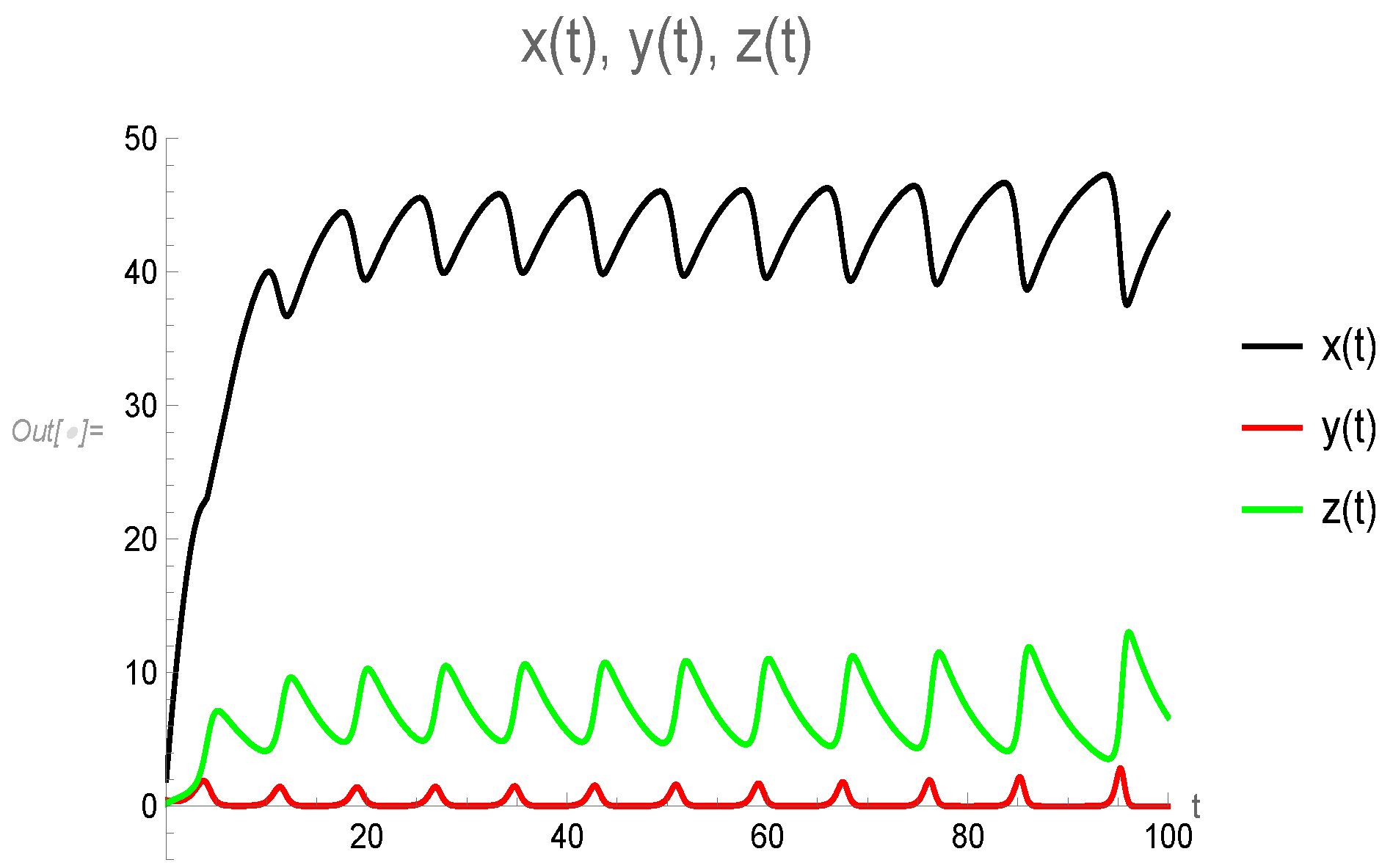
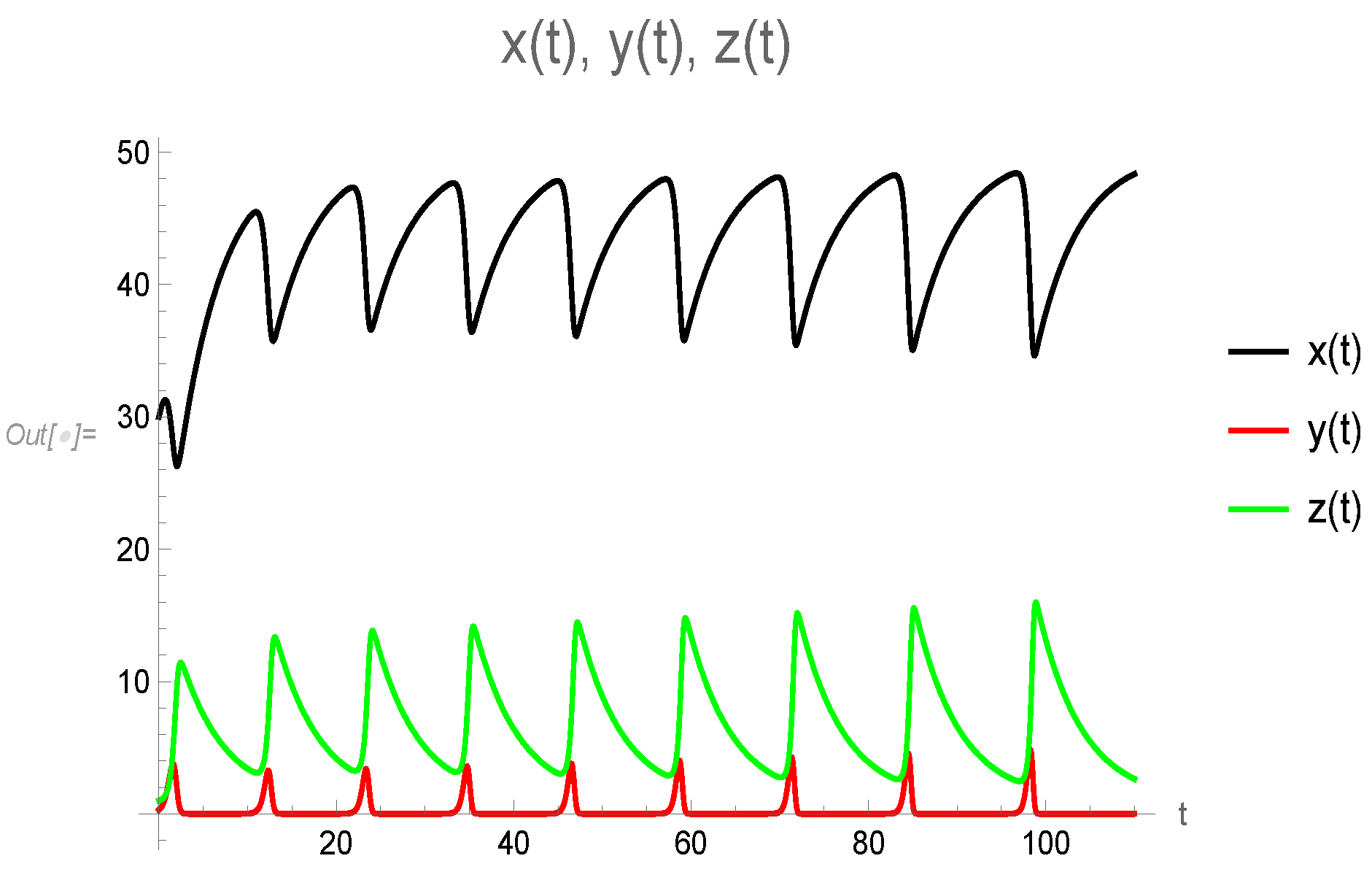
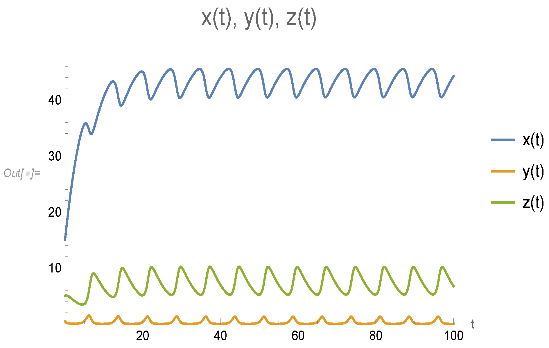
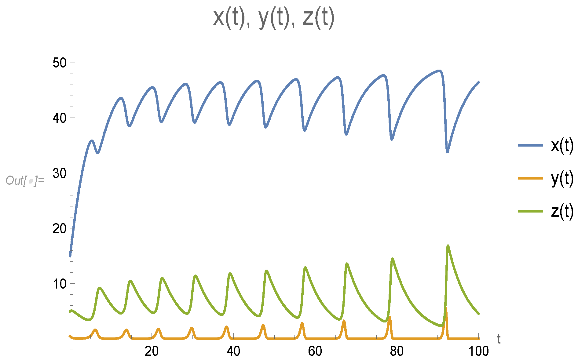
According to Theorem 4, all roots of Equation (11) have negative real parts for all $\tau <{\tau }_0^{+},$ thus $P^{*}$ is locally asymptotically stable for all $\tau <{\tau }_0^{+}.$ When $\tau ={\tau }_0^{+},$ Equation (11) has a pair of purely imaginary roots, and all other roots have negative real parts. Hopf bifurcation occurs as $\tau$ passes across $\tau ={\tau }_0^{+}$. See Figure 1 for solutions to converge to $P^{*}$ for $\tau =0.2<{\tau }_0^{+},$ Figure 2 for Hopf bifurcations to occur and periodic solutions to appear when $\tau ={\tau }_0^{+}=0.440535$, and Figure 3 for solutions blow out when $\tau$ moves to the right of ${\tau }_0^{+}=0.440535.$

2.2. Hopf Bifurcation When $\tau =0$

When $\tau =0,$ Equation (11) becomes

$${\lambda }^2+a_3\lambda +b_3+\eta (c_3\lambda +d_3)e^{-\lambda \rho }=0,$$

(20)

where

$$\begin{array}{ccc}\hfill a_3& =& 2\mu +\delta +\alpha y^{*}-\alpha x^{*},\hfill \\ \hfill b_3& =& \mu (\mu +\alpha y^{*}-\alpha x^{*})+\delta (\mu +\alpha y^{*}),\hfill \\ \hfill c_3& =& z^{*}-y^{*},\hfill \\ \hfill d_3& =& (z^{*}-y^{*})(\mu +\alpha y^{*})+\alpha x^{*}{y}^{*}.\hfill \end{array}$$

(21)

Now, let $\lambda =\omega i$ ($\omega >0$) be a root to Equation (20). When plugged into (20), separating the real and imaginary parts gives

$$\begin{array}{cc}\hfill d_3\eta cos\left(\omega \rho \right)+\eta c_3\omega sin\left(\omega \rho \right)=& {\omega }^2-b_3,\end{array}$$

(22)

$$\begin{array}{cc}\hfill \eta c_3\omega cos\left(\omega \rho \right)-d_3\eta sin\left(\omega \rho \right)=& -a_3\omega .\end{array}$$

(23)

Squaring both sides and adding them together yields

$${\omega }^4+(a_3^2-{\eta }^2{c}_3^2-2b_3){\omega }^2+b_3^2-{\eta }^2{d}_3^2=0.$$

Let $q={\omega }^2$ and denote $a_4=a_3^2-{\eta }^2{c}_3^2-2b_3$ and $b_4=b_3^2-{\eta }^2{d}_3^2.$ Then, the above equation can be rewritten as:

$$q^2+a_{4}q+b_4=0.$$

(24)

Plug $a_3,b_3,c_3$ and $d_3$ given in (21) and $x^{*}$ and $y^{*}$ given in (7) and (8) into $a_4$ and $b_4,$ calculations yield

$$\begin{array}{cc}\hfill a_4=& a_3^2-{\eta }^2{c}_3^2-2b_3=\frac{1}{{(\delta +\eta z^{*})}^2}{Q}_1\left(z^{*}\right),\hfill \end{array}$$

(25)

$$\begin{array}{cc}\hfill b_4=& b_3^2-{\eta }^2{d}_3^2=\frac{(\mu z^{*}-B)}{{(\delta +\eta z^{*})}^4}{Q}_2\left(z^{*}\right)Q_3\left(z^{*}\right),\hfill \end{array}$$

(26)

where $Q_1,Q_2$ and $Q_3$ are polynomials of z, such that

$$\begin{array}{ccc}\hfill Q_1\left(z\right)& =& 2{\eta }^2\mu (\eta -\alpha )z^3+(\mu \left({\alpha }^2\mu -4\alpha \delta \eta +2\delta {\eta }^2\right)+2B{\eta }^2(\alpha -\eta ))z^2\hfill \\ & & -2\left(\delta \mu (\alpha \delta -\eta \mu )+B\left({\alpha }^2\mu -2\alpha \delta \eta +{\eta }^2(\delta -\mu )\right)\right)z\hfill \\ & & +B^2\left({\alpha }^2-{\eta }^2\right)+2\alpha B{\delta }^2+{\delta }^2{\mu }^2,\hfill \end{array}$$

(27)

$$\begin{array}{ccc}\hfill Q_2\left(z\right)& =& \alpha {\delta }^2+\alpha \delta \mu +\alpha B\eta +{\delta }^2\eta +\alpha {\eta }^2{z}^2+{\eta }^3{z}^2+2\alpha \delta \eta z+2\delta {\eta }^{2}z,\hfill \\ \hfill Q_3\left(z\right)& =& -{\eta }^2\mu (\alpha +3\eta )z^3+\eta (2\mu (\alpha \mu -3\delta \eta )+B\eta (\alpha +\eta ))z^2\hfill \\ & & +\delta \mu \left(\alpha \right(\delta +\mu )-3\delta \eta )+B\eta (2\delta \eta -3\alpha \mu )z\hfill \\ & & +B\left({\delta }^2\eta -\alpha \left(-B\eta +{\delta }^2+\delta \mu \right)\right).\hfill \end{array}$$

(28)

Note that $Q_1\left(z\right)$ is a degree three polynomial with $Q_1(B/\mu )=B^2{\eta }^2+2B\delta \eta \mu +{\delta }^2{\mu }^2>0.$ Obviously, $Q_2\left(z^{*}\right)>0,$ and $\mu z^{*}-B>0$ as $z^{*}>B/\mu$ if $R_0>1.$ $Q_3\left(z\right)$ is also a degree three polynomial of z, such that

$$Q_3(B/\mu )=-\frac{2B^3{\eta }^3}{{\mu }^2}-\frac{4B^2\delta {\eta }^2}{\mu }-2B{\delta }^2\eta \le 0$$

and

$$Q_3(B/\mu )<0$$

if $B>0.$

Applying the results of Lemma 2, we have the following results.

Theorem 5.

Let $R_0>1,$ and let $Q_1$ and $Q_3$ be defined by (27), and (28). We then have:

(I)

If $Q_1\left(z^{*}\right)\ge 0$ and $Q_3\left(z^{*}\right)\ge 0$, then Equation (24) has no positive roots.

(II)

If $Q_3\left(z^{*}\right)<0$, or if $Q_3\left(z^{*}\right)=0$ and $Q_1\left(z^{*}\right)<0,$ then Equation (24) has a unique positive root.

Now assume that $R_0>1$ and Equation (24) has at least one positive root. Solving q from Equation (24) for the positive roots gives

$$q^{\pm }=\frac{1}{2}\left[-(a_3^2-{\eta }^2{c}_3^2-2b_3)\pm \sqrt{{(a_3-{\eta }^2{c}_3^2-2b_3)}^2-4(b_3^2-{\eta }^2{d}_3^2)}\right].$$

Note that if Equation (24) has a unique positive root, then it is $q^{+}.$ Let ${\omega }^{\pm }=\sqrt{q^{\pm }}.$ Solving for $sin\left(\omega \rho \right)$ and $cos\left(\omega \rho \right)$ from (22) and (23), we obtain

$$cos\left(\omega \rho \right)=\frac{(d_3-a_3{c}_3){\omega }^2-b_3{d}_3}{\eta \left(c_3^2{\omega }^2+d_3^2\right)}=g_1\left(\omega \right)$$

and

$$sin\left(\omega \rho \right)=\frac{\omega \left(c_3{\omega }^2+a_3{d}_3-b_3{c}_3\right)}{\eta \left(c_3^2{\omega }^2+d_3^2\right)}=g_2\left(\omega \right).$$

Define ${\rho }_n^{\pm },n=0,1,2,\cdots ,$ as

$${\rho }_n^{\pm }=\left\{\begin{array}{cc}\frac{1}{{\omega }^{\pm }}(arccos{g}_1\left({\omega }^{\pm }\right)+2n\pi )\hfill & \mathrm{if}{g}_2\left({\omega }^{\pm }\right)>0,\hfill \\ \frac{1}{{\omega }^{\pm }}(2\pi -arccos{g}_1\left({\omega }^{\pm }\right)+2n\pi )\hfill & \mathrm{if}{g}_2\left({\omega }^{\pm }\right)\le 0.\hfill \end{array}\right.$$

(29)

Hence, ${\rho }_n^{\pm }>0$ and Equation (20) has a pair of purely imaginary roots $\pm i{\omega }^{\pm }$ when $\rho ={\rho }_n^{\pm }$ for $n=0,1,2,\cdots .$ Next, we attempt to establish the transversality condition for Hopf bifurcation. For $\rho >0,$ let

$$\lambda \left(\rho \right)=\alpha \left(\rho \right)+iw\left(\rho \right)$$

(30)

be the root of Equation (20), satisfying

$$\alpha \left({\rho }_n^{\pm }\right)=0,w\left({\rho }_n^{\pm }\right)=w^{\pm }.$$

Differentiating both sides of Equation (20) with respect to $\rho$ gives

$$\begin{array}{c}\hfill \mathrm{Re}{\left(\frac{d\lambda }{d\rho }\right)}_{\rho ={\rho }_n^{\pm }}^{-1}=\frac{\pm \sqrt{a_4^2-4b_4}}{d_3^2+c_3^2{\omega }^2}.\end{array}$$

(31)

Note that $a_4^2-4b_4>0$ since in this case Equation (24) has two positive roots. We thus established that $\mathrm{Re}{\left(\frac{d\lambda }{d\rho }\right)}_{\rho ={\rho }_n^{+}}^{-1}>0$ and $\mathrm{Re}{\left(\frac{d\lambda }{d\rho }\right)}_{\rho ={\rho }_n^{-}}^{-1}<0.$ The discussion above establishes the following stability and Hopf bifurcation results.

Theorem 6.

Assume that $R_0>1$ and let $a_4,b_4,Q_1,Q_3,z^{*},{\omega }^{+},{\rho }_0^{+}$ be defined above. We then have the following results.

(I)

If $Q_1\left(z^{*}\right)\ge 0$ and $Q_3\left(z^{*}\right)\ge 0,$ then all roots of Equation (20) have negative real parts for all delay $\rho \ge 0.$ Therefore, $P^{*}$ is locally asymptotically stable for all $\rho \ge 0.$

(II)

If $Q_3\left(z^{*}\right)<0,$ or if $Q_3\left(z^{*}\right)=0$ and $Q_1\left(z^{*}\right)<0,$ then there is a ${\rho }_0^{+}>0$, such that all roots of Equation (20) have negative real parts for all $\rho \in [0,{\rho }_0^{+})$. It has a pair of purely imaginary roots $\pm i{\omega }^{+}$, and all other roots have negative real parts when $\rho ={\rho }_0^{+}.$ Therefore, $P^{*}$ is locally asymptotically stable for all $\rho <{\rho }_0^{+},$ and is unstable for all $\rho >{\rho }_0^{+}.$ Hopf bifurcation occurs as ρ passes through $\rho ={\rho }_0^{+}$.

If we choose the same parameter values as in Section 2.1, i.e., $A=10,B=0.2$, $\alpha$ = 0.1, $\eta =0.5,\mu =0.2,\delta =0.4.$ Then we have $P^{*}=(43.239,0.3127,7.4479),$ i.e., $z^{*}=7.4479.$ We also have $R_0=4.54545>1,$ and calculations give

$$\begin{array}{ccc}\hfill Q_1\left(z\right)& =& 0.0032+0.0048z-0.0156z^2+0.04z^3,\hfill \\ \hfill Q_3\left(z\right)& =& 0.0132-0.0092z-0.086z^2-0.08z^3.\hfill \end{array}$$

Therefore, $Q_1\left(z^{*}\right)=15.6992,Q_3\left(z^{*}\right)=-37.87<0,$ which means that the condition (II) of Theorem 6 is satisfied, and a ${\rho }_0^{+}>0$ exists. Actually, calculations yield

$${\rho }_0^{+}=0.0474351.$$

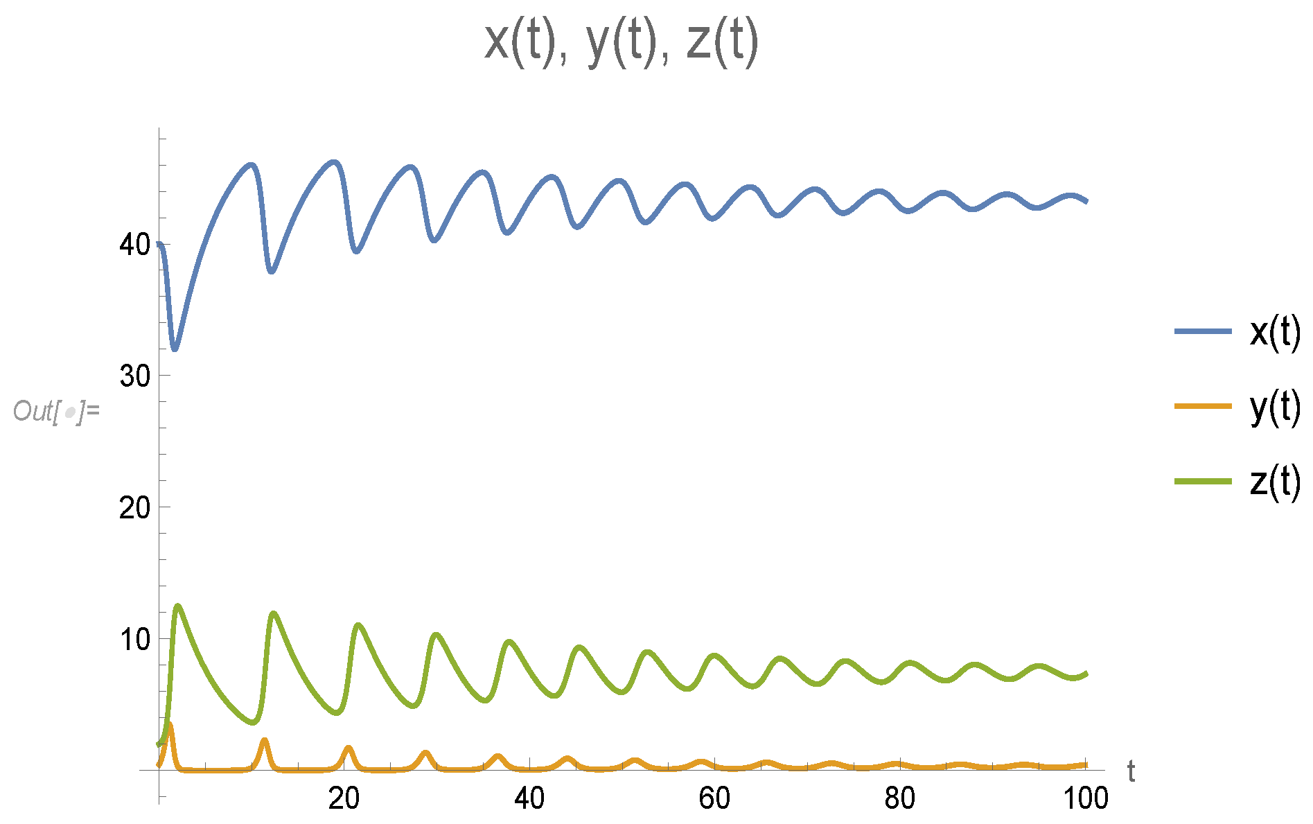
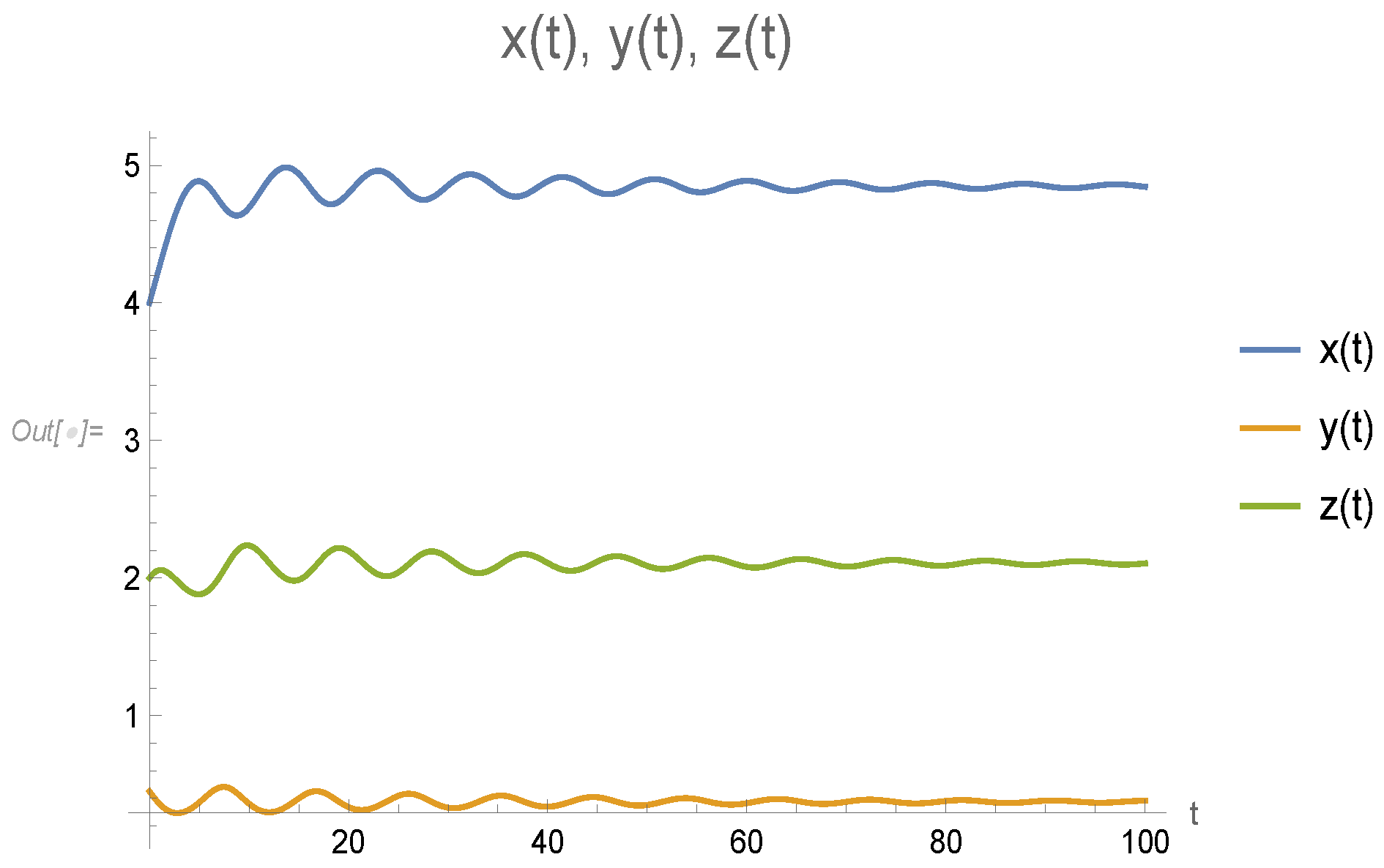
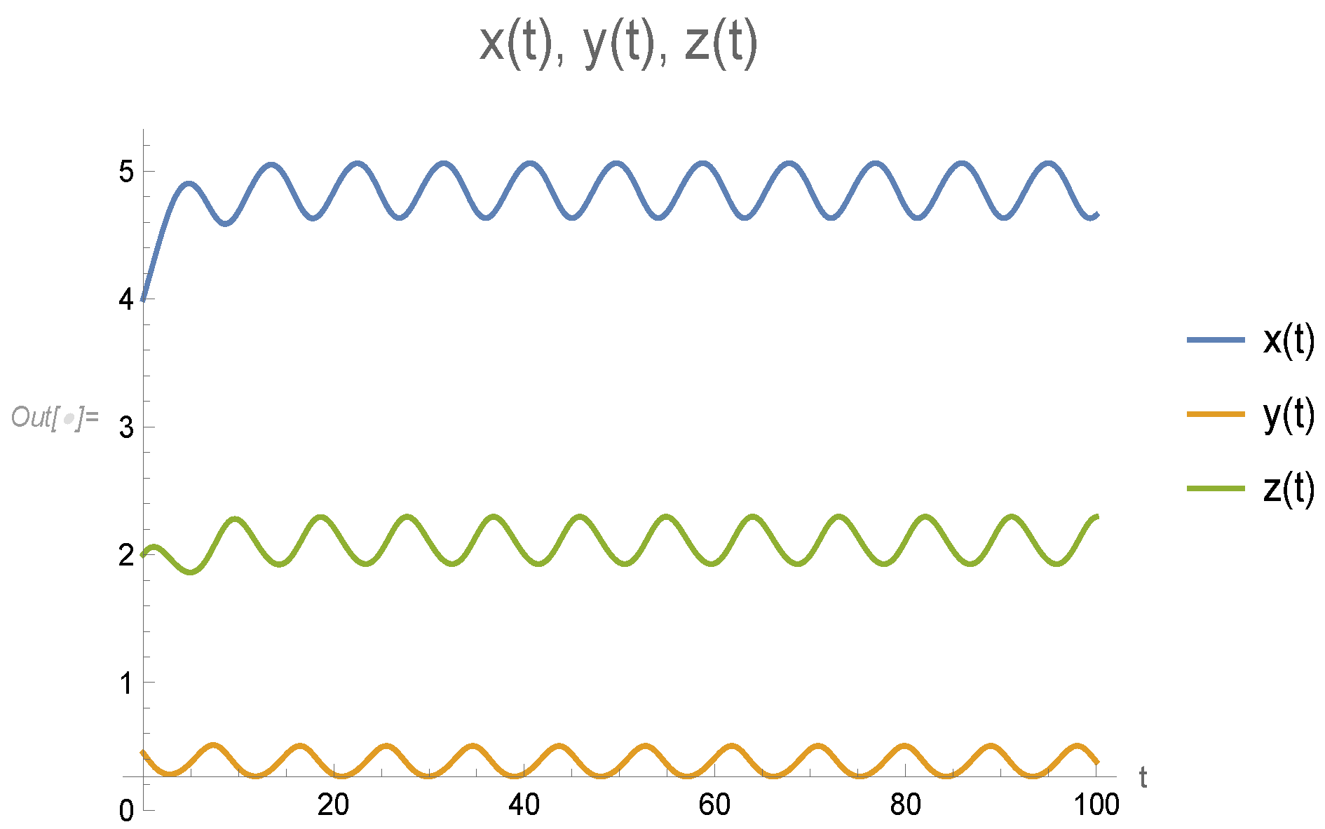
That means that all roots of Equation (20) have negative real parts when $\rho <{\rho }_0^{+};$ therefore, $P^{*}$ is locally asymptotically stable for all $\rho <{\rho }_0^{+}.$ When $\rho ={\rho }_0^{+},$ Equation (20) has a pair of purely imaginary roots, and all other roots have negative real parts. Hopf bifurcation occurs as $\rho$ passes across $\rho ={\rho }_0^{+}$. See Figure 4 for solutions to converge to $P^{*}$ for $\rho =0.02<{\rho }_0^{+},$ Figure 5 for Hopf bifurcations to occur and periodic solutions to appear when $\rho ={\rho }_0^{+}=0.0474351$, and Figure 6 for solutions blow out when $\rho$ moves to the right of ${\rho }_0^{+}=0.0474351$.

2.3. Hopf Bifurcation When $\rho >0$ and $\tau >0$

Now, assume that $\rho \ge 0$ and $\tau \ge 0.$ Let $\lambda =\omega i$ ($\omega >0$) be a root to Equation (11). Plug it into (11), and separate the real and imaginary parts, we obtain

$$\begin{array}{ccc}\hfill c\eta \omega sin\left(\rho \omega \right)+d\eta cos\left(\rho \omega \right)& =& {\omega }^2-b-\delta \omega sin\left(\tau \omega \right)-\delta hcos\left(\tau \omega \right),\hfill \end{array}$$

(32)

$$\begin{array}{ccc}\hfill c\eta \omega cos\left(\rho \omega \right)-d\eta sin\left(\rho \omega \right)& =& -a\omega -\delta \omega cos\left(\tau \omega \right)+\delta hsin\left(\tau \omega \right).\hfill \end{array}$$

(33)

Squaring both sides and adding them together yields

$$\begin{array}{cc}\hfill & 2\delta [\omega \left(ah-b+{\omega }^2\right)sin\left(\tau \omega \right)+({\omega }^2(h-a)-bh)cos\left(\tau \omega \right)]\hfill \\ =\hfill & {\omega }^4+(a^2+{\delta }^2-2b-c^2{\eta }^2){\omega }^2+b^2+h^2{\delta }^2-d^2{\eta }^2\hfill \end{array}$$

which is equivalent to

$$sin(\theta +\omega \tau )=\frac{{\omega }^4+(a^2+{\delta }^2-2b-c^2{\eta }^2){\omega }^2+b^2+h^2{\delta }^2-d^2{\eta }^2}{2\delta \sqrt{(h^2+{\omega }^2)(a^2{\omega }^2+{({\omega }^2-b)}^2)}},$$

where

$$\theta =arcsin\frac{(h-a){\omega }^2-bh}{\sqrt{(h^2+{\omega }^2)(a^2{\omega }^2+{({\omega }^2-b)}^2)}}.$$

Let

$$F\left(\omega \right)=sin(\theta +\omega \tau )$$

(34)

and

$$G\left(\omega \right)=\frac{{\omega }^4+(a^2+{\delta }^2-2b-c^2{\eta }^2){\omega }^2+b^2+h^2{\delta }^2-d^2{\eta }^2}{2\delta \sqrt{(h^2+{\omega }^2)(a^2{\omega }^2+{({\omega }^2-b)}^2)}}.$$

(35)

Now, we study the existence of positive solutions to the equation

$$F\left(\omega \right)=G\left(\omega \right)$$

when $\tau \ge 0.$ First, note that if $\omega =0,$ then we have

$$\frac{(h-a){\omega }^2-bh}{\sqrt{(h^2+{\omega }^2)(a^2{\omega }^2+{({\omega }^2-b)}^2)}}=\frac{-b}{\left|b\right|}=\left\{\begin{array}{cc}\hfill 1,& \mathrm{if}b<0,\hfill \\ \hfill -1,& \mathrm{if}b>0.\hfill \end{array}\right.$$

Therefore, it follows that

$$F\left(0\right)=\left\{\begin{array}{cc}\hfill 1,& \mathrm{if}b<0,\hfill \\ \hfill -1,& \mathrm{if}b>0.\hfill \end{array}\right.$$

we also have

$$G\left(0\right)=\frac{b^2+h^2{\delta }^2-d^2{\eta }^2}{2\delta h\left|b\right|}=\frac{b^2+h^2{\delta }^2}{2\delta h\left|b\right|}-\frac{d^2{\eta }^2}{2\delta h\left|b\right|}$$

and $G\left(\omega \right)\to \infty$ as $\omega \to \infty .$ Also note that F has a sine-shaped curve. If the equation $F\left(\omega \right)=G\left(\omega \right)$ has positive solutions, it has only a finite number of solutions.

Solving Equations (32) and (33) for $cos\left(\omega \rho \right)$ and $sin\left(\omega \rho \right)$, we obtain

$$\begin{array}{cc}\hfill cos\left(\omega \rho \right)& =-\frac{ac{\omega }^2+bd+\delta cos\left(\tau \omega \right)\left(c{\omega }^2+dh\right)+\delta \omega (d-ch)sin\left(\tau \omega \right)-d{\omega }^2}{\eta \left(c^2{\omega }^2+d^2\right)}=h_1\left(\omega \right)\end{array}$$

(36)

$$\begin{array}{cc}\hfill sin\left(\omega \rho \right)& =\frac{ad\omega -bc\omega -\delta sin\left(\tau \omega \right)\left(c{\omega }^2+dh\right)+\delta \omega (d-ch)cos\left(\tau \omega \right)+c{\omega }^3}{\eta \left(c^2{\omega }^2+d^2\right)}=h_2\left(\omega \right).\end{array}$$

(37)

For values of $\tau$, such that $F\left(\omega \right)=G\left(\omega \right)$ has positive roots, assume that $0<{\omega }_1<{\omega }_2<\cdots <{\omega }_m$ are the roots, and define ${\rho }_{jk}^{+},j=1,2,\cdots ,m$, and $k=0,1,2,\cdots ,$ as

$${\rho }_{jk}^{+}=\left\{\begin{array}{ccc}\frac{1}{{\omega }_j}\left[2k\pi +arccos{h}_1\left({\omega }_j\right)\right]\hfill & \mathrm{if}\hfill & h_2\left({\omega }_j\right)>0,\hfill \\ \frac{1}{{\omega }_j}\left[2\pi (k+1)-arccos{h}_1\left({\omega }_j\right)\right]\hfill & \mathrm{if}\hfill & h_2\left({\omega }_j\right)\le 0.\hfill \end{array}\right.$$

(38)

It follows that for every $1\le j\le m,k=0,1,2,\cdots ,$ ${\rho }_{jk}^{+}>0$ is a function of $\tau$ on some interval and for each j, ${\rho }_{jk}^{+}$ are defined on the same interval for all $k.$ There are a number of different cases in terms of functions ${\rho }_{jk}^{+}.$ We list a couple of cases here. For more information regarding the stability regions if a system has two delays, see Hale and Huang [29] and Wang [30].

Theorem 7.

Assume that $R_0>1.$ Let $a,b,c,d,$ and h be defined by (10), and $a_1,b_1,$ and $c_1$ be defined by (13). Also let $F,G$ be defined in (34) and (35). We then have the following results.

(I)

Equation (14) has no positive roots. Then

• If the equation $F\left(\omega \right)=G\left(\omega \right)$ has no positive solutions for any $\tau \ge 0,$ then all roots of Equation (11) have negative real parts for all delays $\rho \ge 0$ and $\tau \ge 0.$ Therefore, $P^{*}$ is locally asymptotically stable for all $\rho \ge 0$ and $\tau \ge 0.$ The stability region of $P^{*}$ is the whole first quadrant of the $(\tau ,\rho )$ plane.
• If the equation $F\left(\omega \right)=G\left(\omega \right)$ has positive solutions for some $\tau \ge 0,$ then there exists a $\rho \left(\tau \right)>0$, such that all roots of Equation (11) have negative real parts for all delays $0\le \rho <\rho \left(\tau \right)$. When $\rho =\rho \left(\tau \right),$ it has a pair of imaginary roots $\pm i\omega$, and all other roots have negative real parts. Therefore, $P^{*}$ is locally asymptotically stable for all $\rho <\rho \left(\tau \right),$ and Hopf bifurcations occur as ρ passes through $\rho \left(\tau \right).$ The stability region of $P^{*}$ is the region given by

  $$\left\{\right(\tau ,\rho ):0\le \tau <\infty ,0\le \rho <\rho (\tau ).\}$$

(II)

Equation (14) has positive roots. Thus, a ${\tau }_0^{+}>0$ exists and is given by (19). Then

• If the equation $F\left(\omega \right)=G\left(\omega \right)$ has no positive solutions for any $0\le \tau <{\tau }_0^{+},$ then all roots of Equation (11) have negative real parts for all delays $\rho \ge 0$ and $0\le \tau <{\tau }_0^{+}.$ Therefore, $P^{*}$ is locally asymptotically stable for all $(\tau ,\rho )$ in the region $\{(\tau ,\rho ):\tau <{\tau }_0^{+},\rho \ge 0\}.$
• If the equation $F\left(\omega \right)=G\left(\omega \right)$ has one positive solution for all $0\le \tau <{\tau }_0^{+},$ then there exists a $\rho \left(\tau \right)>0$, such that all roots of Equation (11) have negative real parts for all delays $(\tau ,\rho )$ in the region $R=\{(\tau ,\rho ):0\le \tau <{\tau }_0^{+},\rho <\rho \left(\tau \right)\}$. When $\rho =\rho \left(\tau \right),$ it has a pair of imaginary roots $\pm i\omega$, and all other roots have negative real parts. Therefore, $P^{*}$ is locally asymptotically stable for all $(\tau ,\rho )$ in $R,$ and Hopf bifurcations occur as $(\tau ,\rho )$ crosses through the curve given by $\rho =\rho \left(\tau \right).$

Again, we perform some numerical simulations to illustrate our theoretical results. First, if we choose the same parameter values as in Section 2.1 and Section 2.2 as $A=10$, $B=0.2$, $\alpha =0.1,\eta =0.5,\mu =0.2,\delta =0.4.$ Then, we have $P^{*}=(43.239,0.3127,7.4479),$ $R_0=4.54545>1$. In this case, both ${\tau }_0^{+}>0$ and ${\rho }_0^{+}>0$ exist, and they are

$${\tau }_0^{+}=0.440535,{\rho }_0^{+}=0.047453.$$

A function $\rho \left(\tau \right)>0$ as a function of $\tau$ can be found using (38), such that the stability region S in the $\tau \rho$-space can be identified. $P^{*}$ is locally asymptotically stable for all $(\tau ,\rho )$ in the interior of $S,$ and Hopf bifurcation occurs as $(\tau ,\rho )$ passes across the boundary of $S,$ where

$$S=\{(\tau ,\rho ):0\le \tau \le {\tau }_0^{+},0\le \rho \le \rho \left(\tau \right)\}.$$

See Figure 7 for the stability region S and Figure 8 for solutions to converge to $P^{*}$ when $(\tau ,\rho )=(0.1,0.1)$ is in the interior of $S.$ Also see Figure 9 for Hopf bifurcations to occur and periodic solutions to appear when $(\tau ,\rho )=(0.2,0.0314633)$ is on the boundary of the stability region S, and Figure 10 for solutions blow out when $(\tau ,\rho )$ moves out of the stability region S.

Next, if we choose the parameter values as $A=2,B=0.2,\alpha =0.3,\eta =0.5$, $\mu$ = 0.3, $\delta =0.1,$ then we have $P^{*}=(4.8471,0.37484,2.1094),$ and $R_0=2.72727>1.$ In this case, calculations show that:

$$a_2=0.629726,b_2=0.0992197.$$

So, Equation (14) has no positive roots, and that implies that ${\tau }_0^{+}>0$ does not exist. But in this case, ${\rho }_0^{+}>0$ exists, and

$${\rho }_0^{+}=0.325204.$$

A function of $\rho \left(\tau \right)>0$ as a function of $\tau$ can be found using (38), such that the stability region S in the $\tau \rho$-space can be identified. $P^{*}$ is locally asymptotically stable for all $(\tau ,\rho )$ in the interior of $S;$ Hopf bifurcation occurs as $(\tau ,\rho )$ passing across the boundary of $S,$ where

$$S=\left\{\right(\tau ,\rho ):0\le \tau ,0\le \rho \le \rho (\tau \left)\right\}$$

See Figure 11 for the stability region S, Figure 12 for solutions to converge to $P^{*}$ when $(\tau ,\rho )=(0.1,0.1)$ is in the interior of $S,$ and Figure 13 for Hopf bifurcations to occur and periodic solutions to appear when $(\tau ,\rho )=(1,0.2413)$ is on the boundary of the stability region S. As $(\tau ,\rho )$ moves out of the stability region S, solutions will blow out to infinity. It’s similar to cases above, so we omit a numerical simulation here.

3. Discussion

In this paper, we introduced and explored a mathematical model for online social networks, wherein the population is categorized into three distinct sub-classes: potential network users, active users, and individuals opposed to networks. Diverging from existing literature, our model accounts for the presence of individuals who will never express interest in using online networks. Additionally, active online social network users may exhibit a tendency to lose interest and subsequently abandon the platform over time, with or without interacting with non-users.

Assuming that the basic reproduction number $R_0$ exceeds unity, we delved into an investigation of whether time delays affecting active users’ abandonment of the network can induce a switch in the stability of the unique user prevailing equilibrium (UPE) denoted as $P^{*}$. We established conditions ensuring the asymptotic stability of $P^{*}$ for all delays $\tau \ge 0$ and $\rho \ge 0$, enabling individuals across all three sub-classes to settle into equilibrium over time. Furthermore, we identified stability regions and associated conditions under which Hopf bifurcations occur as the delays $(\tau ,\rho )$ traverse the boundaries of these regions. Consequently, periodic solutions emerged, leading to oscillations in the populations of the three sub-classes.

To validate our theoretical findings, we conducted numerical simulations, providing empirical evidence to support the dynamics predicted by our model. Through this comprehensive analysis, we shed light on the complex dynamics inherent in online social networks and elucidate the role of time delays in shaping equilibrium states and oscillatory behavior. Our study contributes to a deeper understanding of the underlying mechanisms driving the evolution of online social networks, with implications for diverse fields including sociology, network science, and computational modeling.

References

- Bettencourt, L.M.; Cintrn-Arias, A.; Kaiser, D.I.; Castillo-Chvez, C. The power of a good idea: Quantitative modeling of the spread of ideas from epidemiological models. Phys. A Stat. Mech. Its Appl. 2006, 364, 513–536. [Google Scholar] [CrossRef]
- Cannarella, J.; Spechler, J. Epidemiological modeling of online network dynamics. arXiv 2014, arXiv:1401.4208. [Google Scholar]
- Chen, R.; Kong, L.; Wang, M. Stability analysis of an online social network model. Rocky Mt. J. Math. 2003, 53, 1019–1041. [Google Scholar] [CrossRef]
- Dai, G.; Ma, R.; Wang, H.; Wang, F.; Xu, K. Partial differential equations with Robin boundary conditions in online social networks. Discret. Contin. Dyn. Syst. Ser. B 2015, 20, 1609–1624. [Google Scholar] [CrossRef]
- Graef, J.R.; Kong, L.; Ledoan, A.; Wang, M. Stability analysis of a fractional online social network model. Math. Comput. Simulat. 2020, 178, 625–645. [Google Scholar] [CrossRef]
- Kong, L.; Wang, M. Deterministic and stochastic online social network models with varying population size. Dcdis Ser. A Math. Anal. 2023, 30, 253–275. [Google Scholar]
- Kong, L.; Wang, M. Optimal control for an ordinary differential equation online social network model. Differ. Equ. Appl. 2022, 14, 205–214. [Google Scholar] [CrossRef]
- Lei, C.; Lin, Z.; Wang, H. The free boundary problem describing information diffusion in online social networks. J. Differ. Equ. 2013, 254, 1326–1341. [Google Scholar] [CrossRef]
- Liu, X.; Li, T.; Cheng, X.; Liu, W.; Xu, H. Spreading dynamics of a preferential information model with hesitation psychology on scale-free networks. Adv. Differ. Equ. 2019, 2019, 279. [Google Scholar] [CrossRef]
- Liu, X.; Li, T.; Tian, M. Rumor spreading of a SEIR model in complex social networks with hesitating mechanism. Adv. Differ. Equ. 2018, 2018, 391. [Google Scholar] [CrossRef]
- Wang, F.; Wang, H.; Xu, K. Diffusion logistic model towards predicting information diffusion in online social networks. In Proceedings of the 2012 32nd International Conference on Distributed Computing Systems Workshops (ICDCSW), Macau, China, 18–21 June 2012; pp. 133–139. [Google Scholar]
- Anderson, R.M.; May, R.M. Population biology of infectious diseases: Part I. Nature 1979, 280, 361–367. [Google Scholar] [CrossRef] [PubMed]
- Bernoussi, A. Stability analysis of an SIR epidemic model with homestead-isolation on the susceptible and infectious, immunity, relapse and general incidence rate. Int. J. Biomath. 2023, 16, 2250102. [Google Scholar] [CrossRef]
- Han, Z.; Wang, Y.; Gao, S.; Sun, G.; Wang, H. Final epidemic size of a two-community SIR model with asymmetric coupling. J. Math. Biol. 2024, 88, 51. [Google Scholar] [CrossRef] [PubMed]
- Hill, A.; Glasser, J.; Feng, Z. Implications for infectious disease models of heterogeneous mixing on control thresholds. J. Math. Biol. 2023, 86, 53. [Google Scholar] [CrossRef]
- Li, A.; Zou, X. R0 May Not Tell Us Everything: Transient Disease Dynamics of Some SIR Models Over Patchy Environments. Bull. Math. Biol. 2024, 41. [Google Scholar] [CrossRef] [PubMed]
- Kermack, W.; McKendrick, A. A Contribution to the Mathematical Theory of Epidemics. Proc. R. Soc. Lond. Ser. A Contain. Pap. Math. Phys. Character 1927, 115, 700–721. [Google Scholar]
- Li, M.Y.; Graef, J.R.; Wang, L.; Karsai, J. Global dynamics of an SEIR model with vertical transmission. SIAM J. Appl. Math. 1999, 160, 191–213. [Google Scholar] [CrossRef]
- Li, M.Y.; Smith, H.L.; Wang, L. Global dynamics of a SEIR model with a varying total population size. Math. Biosci. 2001, 62, 58–69. [Google Scholar] [CrossRef]
- Llibre, J.; Salhi, T. Phase portraits of an SIR epidemic model. Appl. Anal. 2024, 103, 1165–1175. [Google Scholar] [CrossRef]
- Wang, L.; Li, M.Y.; Kirschner, D. Mathematical analysis of the global dynamics of a model for HTLV-I infection and ATL progression. Math. Biosci. 2002, 179, 207–217. [Google Scholar] [CrossRef]
- Wang, L.; Wu, X. Stability and Hopf Bifurcation for an SEIR Epidemic Model with Delay. Adv. Theory Nonl. Anal. Its Appl. 2018, 2, 113–127. [Google Scholar] [CrossRef]
- Xie, J.; Guo, H.; Zhang, M. Dynamics of an SEIR model with media coverage mediated nonlinear infectious force. Math. Biosci. Eng. 2023, 20, 14616–14633. [Google Scholar] [CrossRef] [PubMed]
- Zhang, J.; Qiao, Y. Bifurcation analysis of an SIR model considering hospital resources and vaccination. Math. Comput. Simul. 2023, 208, 157–185. [Google Scholar] [CrossRef]
- Barman, M.; Mishra, N. Hopf bifurcation analysis for a delayed nonlinear-SEIR epidemic model on networks. Chaos Solitons Fractals 2024, 178, 114351. [Google Scholar] [CrossRef]
- Barman, M.; Mishra, N. Hopf bifurcation in a networked delay SIR epidemic model. J. Math. Anal. Appl. 2023, 525, 127131. [Google Scholar] [CrossRef]
- Wang, L.; Wang, M. Stability and Bifurcation Analysis For An OSN Model with Delay. Adv. Theory Nonl. Anal. Its Appl. 2023, 7, 413–427. [Google Scholar] [CrossRef]
- Ruan, S.; Wei, J. On the zeros of transcendental functions with applications to stability of delay differential equations with two delays. Dyn. Contin. Discret. Impuls. Syst. 2003, 10, 863–874. [Google Scholar]
- Hale, J.; Huang, W. Global geometry of the stable regions for two delay differential equations. Math. Anal. Appl. 1993, 178, 344–362. [Google Scholar] [CrossRef]
- Wang, L. Stability and bifurcation analysis for a general differential equation with two delays. Pan-Am. Math. J. 2021, 31, 55–78. [Google Scholar]
Figure 1.
Solutions converge to
Figure 2.
Periodic solutions appear.
Figure 3.
Solutions go to infinity.
Figure 4.
Figure 5.
Figure 6.
Figure 7.
The stability region.
Figure 8.
Figure 9.
is on the boundary of Periodic solutions appear.
Figure 10.
is outside of Solutions go to infinity.
Figure 11.
Figure 12.
Figure 13.
Disclaimer/Publisher’s Note: The statements, opinions and data contained in all publications are solely those of the individual author(s) and contributor(s) and not of MDPI and/or the editor(s). MDPI and/or the editor(s) disclaim responsibility for any injury to people or property resulting from any ideas, methods, instructions or products referred to in the content. |
© 2024 by the authors. Licensee MDPI, Basel, Switzerland. This article is an open access article distributed under the terms and conditions of the Creative Commons Attribution (CC BY) license (https://creativecommons.org/licenses/by/4.0/).
Share and Cite
MDPI and ACS Style
Wang, L.; Wang, M. Bifurcation Analysis for an OSN Model with Two Delays. Mathematics 2024, 12, 1321. https://0-doi-org.brum.beds.ac.uk/10.3390/math12091321
AMA Style
Wang L, Wang M. Bifurcation Analysis for an OSN Model with Two Delays. Mathematics. 2024; 12(9):1321. https://0-doi-org.brum.beds.ac.uk/10.3390/math12091321
Chicago/Turabian StyleWang, Liancheng, and Min Wang. 2024. "Bifurcation Analysis for an OSN Model with Two Delays" Mathematics 12, no. 9: 1321. https://0-doi-org.brum.beds.ac.uk/10.3390/math12091321
Note that from the first issue of 2016, this journal uses article numbers instead of page numbers. See further details here.