
Mining Trajectory Planning of Unmanned Excavator Based on Machine Learning
by
Zhong Jin
1,2, 
Mingde Gong
1,*,
Dingxuan Zhao
1,
Shaomeng Luo
2,
Guowang Li
2,
Jiaheng Li
2,
Yue Zhang
1 and
Wenbin Liu
1 1
School of Mechanical Engineering, Yanshan University, Qinhuangdao 066004, China
2
Guangxi Liugong Machinery Co., Ltd., Liuzhou 545007, China
*
Author to whom correspondence should be addressed.
Mathematics 2024, 12(9), 1298; https://0-doi-org.brum.beds.ac.uk/10.3390/math12091298
Submission received: 23 March 2024
/
Revised: 19 April 2024
/
Accepted: 20 April 2024
/
Published: 25 April 2024
Abstract
:Trajectory planning plays a crucial role in achieving unmanned excavator operations. The quality of trajectory planning results heavily relies on the level of rules extracted from objects such as scenes and optimization objectives, using traditional theoretical methods. To address this issue, this study focuses on professional operators and employs machine learning methods for job trajectory planning, thereby obtaining planned trajectories which exhibit excellent characteristics similar to those of professional operators. Under typical working conditions, data collection and analysis are conducted on the job trajectories of professional operators, with key points being extracted. Machine learning is then utilized to train models under different parameters in order to obtain the optimal model. To ensure sufficient samples for machine learning training, the bootstrap method is employed to adequately expand the sample size. Compared with the traditional spline curve method, the trajectories generated by machine learning models reduce the maximum speeds of excavator boom arm, dipper stick, bucket, and swing joint by 8.64 deg/s, 10.24 deg/s, 18.33 deg/s, and 1.6 deg/s, respectively; moreover, the error does not exceed 2.99 deg when compared with curves drawn by professional operators; and, finally, the trajectories generated by this model are continuously differentiable without position or velocity discontinuities, and their overall performance surpasses that of those generated by the traditional spline curve method. This paper proposes a trajectory generation method that combines excellent operators with machine learning and establishes a machine learning-based trajectory-planning model that eliminates the need for manually establishing complex rules. It is applicable to motion path planning in various working conditions of unmanned excavators.
MSC:
00A06; 68T071. Introduction
Trajectory planning is a crucial technology in unmanned excavators, and a well-designed motion trajectory significantly influences the control effectiveness of these machines. Current research on trajectory generation primarily focuses on three aspects: (1) generating trajectories using high-order curves based on physical constraint points and other constraints; (2) fitting artificial operation curves, with a particular emphasis on bucket tip position trajectory fitting; and (3) generating trajectories based on force and torque feedback, with an emphasis on excavation action trajectory planning. YOO et al. [1] proposed generating motion trajectories using B-spline curves constrained by the maximum pump flow rate. ZOU et al. [2] also utilized B-spline curves combined with constraint conditions to generate three types of excavation trajectories: shortest time, minimum energy, and minimum operating force. JUD et al. [3] achieved results similar to those of operators through end-effector force-torque path planning and later adopted cubic Hermite spline curves for continuous excavation path planning [4]. KIM et al. [5] designed two different operational paths based on the shortest operating time and the minimum torque, respectively. GROLL et al. [6] divided the operational motion into segments and established sub-modules for each stage to form a complete trenching process. LEE et al. [7] divided tasks into three stages, completed path planning under global planner, and utilized model-predictive control (MPC) to update local path information in real-time. ZHANG et al. [8] added acceleration jerk constraints and used a sequential quadratic programming algorithm to calculate optimal decision-making solutions; ZHAO et al. [9] established topologically equivalent paths to ensure smooth excavation processes; and FENG H. et al. [10] decomposed trenching operations.
Due to its exceptional adaptability to nonlinear processes, machine learning has been extensively employed in the domain of unmanned excavators. PARK et al. [11] utilized echo-state networks for generating excavator models. ZHOU et al. [12] and OGUMA et al. [13] employed neural networks for diagnosing excavator faults, and the mechanical performance of excavators was predicted using a similar approach by Seker et al. [14]. KURINOV et al. [15] accomplished the automatic loading of excavators through reinforcement learning within a simulation environment, and the study conducted by Samtani et al. [16] also employed reinforcement learning techniques to develop Dueling Double Deep-Q Networks and extensively investigated the fracturing actions of excavators. Through data-driven approaches, task planning research was conducted by ZHAO et al. [9], and inverse motion control of excavator models was conducted by Lee et al. [17]. EGLI et al. [18] trained models using reinforcement learning techniques to accurately identify soil hardness, while YU et al. [19] integrated physical and data-driven models for real-time soil resistance prediction. Li et al. [20] also employed a hybrid approach that integrates kinematic modeling and machine learning techniques to accurately predict resistance. GUO et al. [21], on the other hand, simulated operator’s operating patterns using deep neural networks. By leveraging the well-established applications of image analysis in deep learning, OSA T et al. [22] investigated mining tasks through deep image learning techniques, while Kim et al. [23] developed a visual-based model for recognizing mining actions in job statistics. On the other hand, YAO et team [24] generated continuous excavation trajectories employing PINN. Furthermore, ZHAO et al. [25] also discovered that, under optimally planned trajectories, the fluctuation of excavation angles in unmanned excavators is greater than that observed during manual operations.
Based on the comprehensive research mentioned above, the current challenge in trajectory planning for work devices is as follows: the effectiveness of trajectory planning relies solely on the quality of established planning rules, often limited to fulfilling specific optimal objectives without considering holistic outcomes [26]. Presently, most studies concentrate on singular objectives [27] (e.g., minimizing energy consumption) for job trajectory planning, posing difficulties in balancing multiple objectives (such as minimizing time, reducing energy consumption, and mitigating impact). Trajectory planning that prioritizes specific objectives typically compromises other parameter characteristics and encounters practical implementation challenges.
In response to the aforementioned issues, this study proposes a trajectory planning method that integrates the exceptional operator’s operational trajectory with machine learning. During long-term practical operations, skilled operators have developed an operating style intuitive and challenging to precisely describe, which is continuously fine-tuned to achieve a balance among multiple objectives. Therefore, it is imperative to employ machine learning techniques for analyzing the operator’s operational trajectory and establishing a model that generates optimal operation trajectories aligning with the overall characteristics while considering multiple objectives. This paper initially describes and models traditional trajectory generation methods, followed by collecting and analyzing professional operator’s operational data while expanding the sample size using a bootstrap method [28]. Subsequently, machine learning is applied for model training in order to obtain the final trajectory-planning model. Finally, a comparative analysis of differences in the trajectory characteristics between machine learning model trajectories, professional operator trajectories, and traditional spline curve-based trajectory planning is conducted. The results demonstrate that, in terms of consistency and continuity, among other aspects, the machine learning model can generate high-quality operating trajectories similar to those of exceptional operators while surpassing conventional trajectory planning methods.
2. Sample Methods
2.1. Traditional Trajectory Generation
Excavator trajectory planning is a crucial part of motion planning for unmanned excavators, and its core lies in accurately planning the movement trajectory of the excavator arm from the starting position to the target position, as well as intermediate positions, based on the task requirements. Typically, we use spline curves for representation. Spline curves possess characteristics such as simplicity, ease of use, continuity, and controllability of start and endpoints, making them highly suitable for generating excavation trajectories [29]. By treating n key points as the segment points and adding appropriate control points to achieve the segmented fitting of joint movements [30,31], corresponding excavation trajectories can be generated.
As an illustration of trajectory generation for dynamic boom joint angles, the breakpoints are presented below.
Among them, Tboom represents the time coordinate points of the trajectory, while Θboom denotes the angular coordinate points of the trajectory.
The calculation of trajectory control points can be formulated according to the following equation:
Among them, Aboom and Bboom are control point matrix coefficients, with the specific form shown below.
Similarly, the control points for trajectory generation of the arm joint, bucket joint, and swing joint can be obtained as illustrated below.
The coefficient matrix exhibits the same structure as the dynamic arm matrix, and its specific values should be suitably adjusted in accordance with practical circumstances. However, further elaboration on this matter is beyond the scope of this discussion.
The excavation trajectory of each joint can be precisely fitted by employing a segmented cubic Bézier spline curve. The operator’s operation trajectory can be effectively segmented, enabling a seamless fit of all curve types, including straight lines, through the utilization of cubic Bézier curves. Consequently, the expressions for each joint’s trajectories can be standardized as cubic Bézier curves.
The mathematical representation of a third-order Bézier curve is as follows:
In addition to the two known endpoints, each segment of the trajectory that requires fitting necessitates the inclusion of two additional intermediate points as the control points. As these newly added points do not lie on the trajectory itself, it becomes imperative to adjust the aforementioned control matrix coefficients based on both the trend of trajectory changes and the characteristics inherent to Bézier curves. Once the key points are determined for a given operator excavation trajectory, the corresponding joint trajectories can be generated using the aforementioned control point formula.
2.2. Professional Operator Data Collection and Analysis
The generation of excavation trajectories must consider multiple factors, including power characteristics, workspace limitations, motion time, and path smoothness of the excavators. However, commonly used point-fitting methods currently struggle to comprehensively account for these diverse factors. In practical operations, professional operators often exhibit optimized and efficient characteristics when operating excavators, making them suitable templates for unmanned excavators. In this section, we employ the bootstrap method to expand their excavation trajectories as samples based on data from professional operators and utilize them as inputs for machine learning algorithms to generate excavation trajectories.
In order to ensure the standardization and reproducibility of professional operators’ actions, this article presents comprehensive specifications for the operators, work scenarios, and objects involved in the operations.
Two individuals engaged in the occupation of excavator-testing operators, with five years of experience in operating excavators. They were 38 years old and male, reaching an expert level in terms of operational skills.
Excavators are standardized batch products, devoid of any modifications or customizations. Only when executing trajectory tracking control, additional computational controller hardware is incorporated and integrated into the primary machine controller. The parameters for each joint can be found in the table provided (Table 1).
The task scenario involves excavation and loading on a high platform, with the angles of excavation and unloading being approximately 90 degrees.
The target for the excavation is fine sand characterized by a low water content, absence of compaction, and a uniform particle size. As depicted in Figure 1, the fine sand exhibits a distinct morphology that is closely associated with the positioning of vehicles.
To ensure the consistency of the operator data collected during the operations, it is required that the operators refrain from moving the excavator tracks and only perform rotation, excavation, and unloading actions. Operator 1 conducted a series of 20 consecutive excavation and unloading operations before site restoration, followed by Operator 2 performing excavation operations under identical conditions. The real-time collection of operational trajectory data was carried out for both operators. After eliminating significant differences in the data curves, a final set of 19 valid excavation data points were obtained for Operator 1, while Operator 2 yielded 12 valid sets.
2.3. Sample Expansion
A substantial volume of raw data is imperative for attaining optimal training outcomes in machine learning. However, amassing an extensive dataset of operator operation curves proves to be neither cost-effective nor practical. Hence, a viable approach to tackle this issue lies in sample augmentation. Currently, there exist several methods for augmenting small samples, including the random sequence method, the recursive interpolation method, the offset method, the SMOTE method, the Monte Carlo method, and the bootstrap resampling method. Among these techniques, except for bootstrap resampling, other sample augmentation methods have certain limitations, such as the requirement to determine the distribution characteristics of the samples. However, unlike other approaches, bootstrap resampling demonstrates a broader applicability as it does not necessitate specific distribution characteristics of the samples.
The principle of bootstrap capacity expansion is briefly outlined as follows [32].
Firstly, arrange the initial samples in a sorted manner and subsequently generate regenerated samples using the following formula:
Among them,
δ is uniformly distributed random numbers in [0, 1];
is the i-th original sample value.
After undergoing standardization processing using Matlab, this method has been encapsulated into the bootstrp() function for direct implementation. The function exclusively supports the expansion of one-dimensional samples, necessitating the conversion of the operator’s two-dimensional data into a one-dimensional format. After analyzing the operator’s operation curve, we have determined that utilizing two parameters, namely, task cycle and joint angle range, would effectively reduce the data dimensions. Utilizing the reduced dataset, we independently expand both the task cycle and joint angle range. Subsequently, new sample curves are generated by applying the expanded data to the original curve.
The dataset of job cycle samples and joint angle amplitude after expansion is shown below (Figure 2).
The new sample curve, depicted in the figure below, was obtained by combining expanded samples with the original samples (Figure 3).
2.4. Generate Mining Trajectories
Machine learning is currently an increasingly mature solution. Several scholars have already conducted research on motion trajectory generation using machine learning techniques [15,16,20,23,33,34]. However, this paper distinguishes itself by employing bootstrap resampling [32] to augment the operator’s limited sample data, resulting in relatively conservative yet diverse samples. Subsequently, training is carried out based on key points to generate the final trajectory model.
2.4.1. Key Point Selection
The coordinate system of an excavator is defined as illustrated in the diagram. The machine coordinate system (x0, y0, z0) has its origin located at the pivot center and at the same height as the lower hinge point of the boom. Within this machine coordinate system, distinct coordinate systems are established for the boom (x1, y1, z1), arm (x2, y2, z2), and bucket (x3, y3, z3). The angles of the boom, arm, and bucket are all relative values that increase in a counterclockwise direction. The swing angle is determined based on the current posture, with positive increments considered when rotating clockwise (Figure 4).
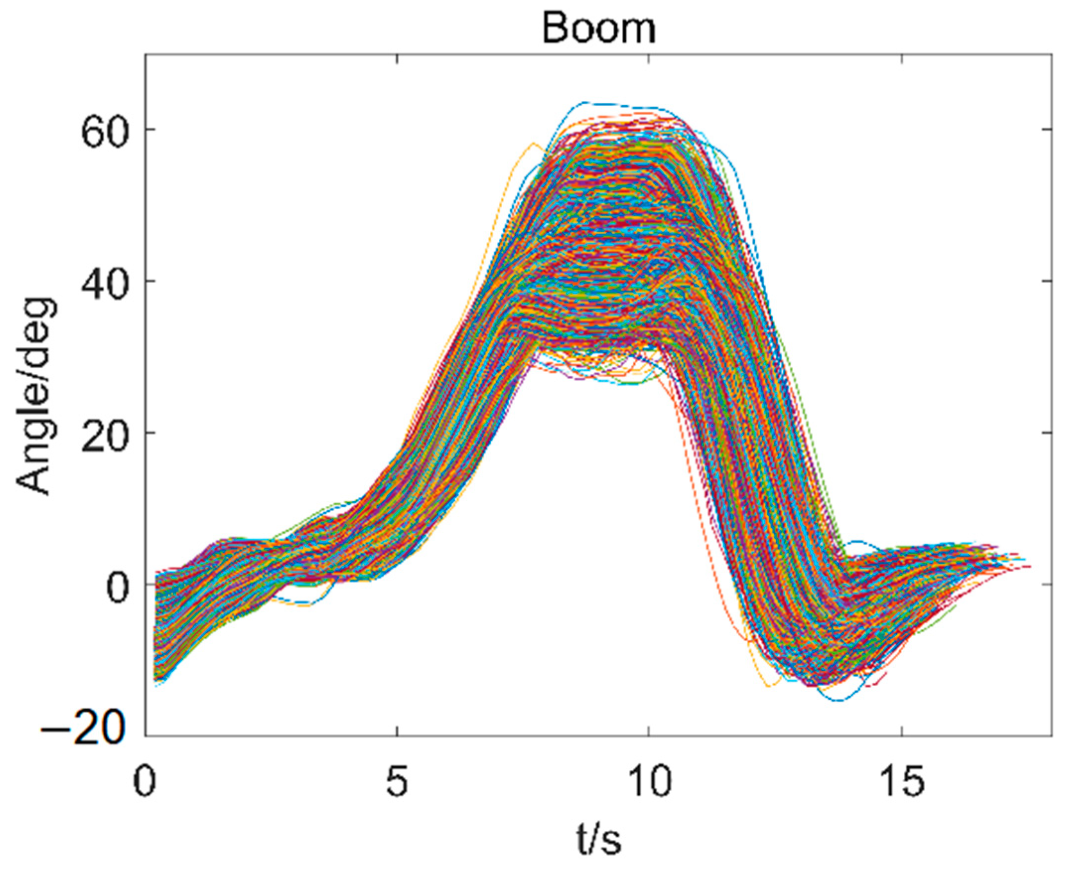
By analyzing the spatial motion trajectory of the excavator bucket tip in the machine coordinate system, as well as the individual motion trajectories of its four joints, we have chosen to focus our research on the most representative curves of these four joints. The accompanying diagram presents contour plots depicting these joint trajectories during operations conducted by two skilled operators. From these motion trajectory curves, it can be observed that both operators’ work paths exhibit overall similarity while also displaying distinct personal characteristics. For instance, in terms of arm trajectory, Operator 1 demonstrates a comparatively slower lifting speed compared to Operator 2; however, their boom lowering speed is relatively faster. In contrast, Operator 2 exhibits a higher level of consistency when reaching maximum angles—a quality noticeably absent in Operator 1’s curve (Figure 5).
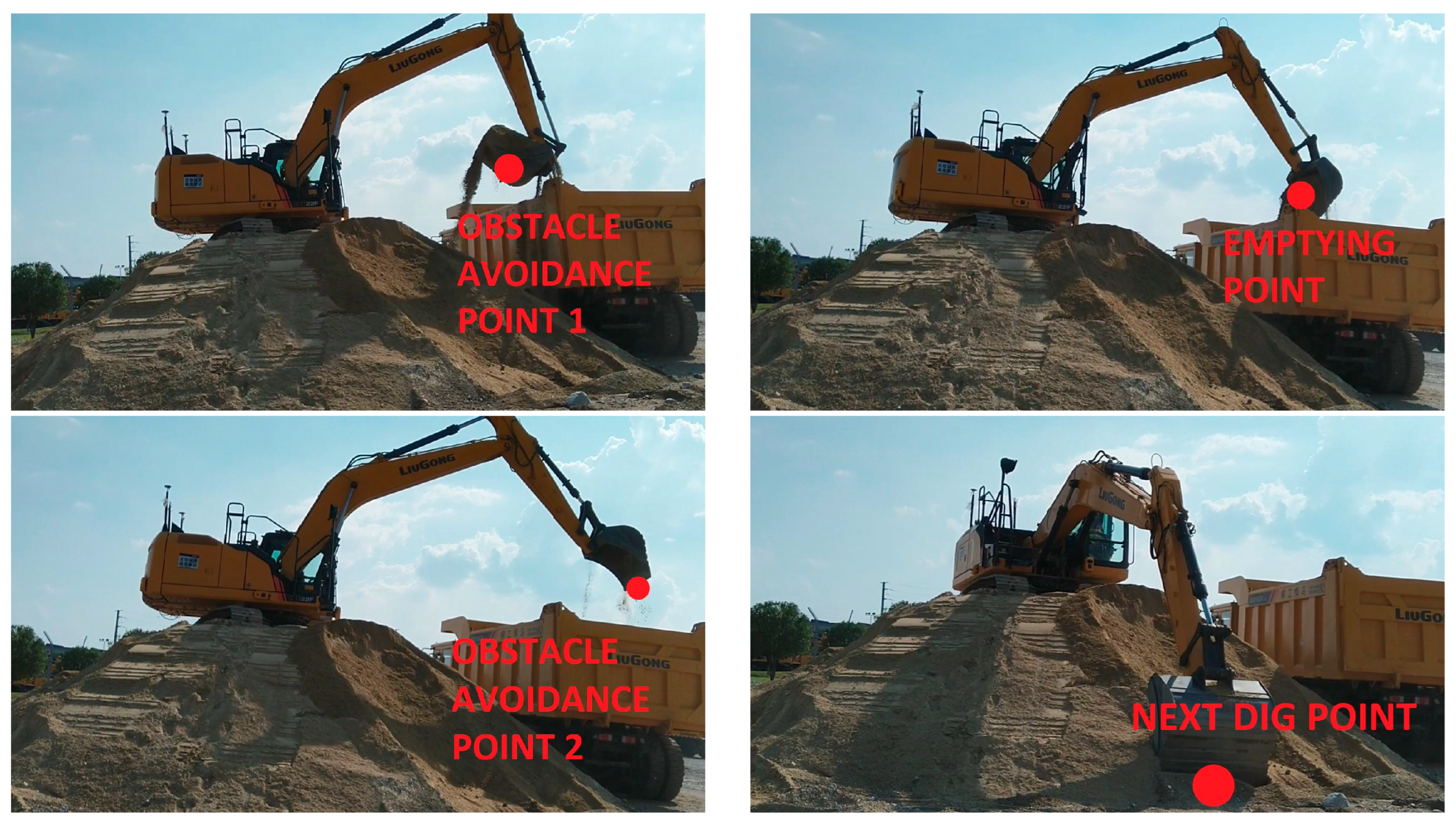
During excavation operations, the operator must precisely execute six key points while allowing for flexible adjustments in intermediate steps as needed. The sequence of these fixed key points includes the starting and ending excavation points, two obstacle avoidance points, an unloading point, and the next excavation point. Although minor differences may occur due to safety space considerations made by the operator during each operation cycle, these six key points are relatively consistent. The diagram below illustrates their positions (Figure 6).
Based on the curves of the four joint angles, the positions of the six key points can be determined, as illustrated in the diagram provided below (Figure 7).
The spatial coordinates of each key point can be acquired through perception or pre-determined methods and are presented as known conditions in this paper. The four joint angle values corresponding to the coordinates of each key point can be obtained through robot inverse kinematics solving, which will not be further expounded upon within the scope of this paper.
The temporal coordinates of the key points are also crucial factors in acquiring a reasonable trajectory; however, these temporal coordinates cannot be directly obtained. By observing the operational curves of two operators, certain principles can be inferred to serve as the foundation for calculating the corresponding temporal coordinates of each key point.
Guideline 1: The excavator arm should retract at a consistent speed from the excavation point to the endpoint.
Guideline 2: Upon reaching the endpoint, the boom should briefly pause before lifting uniformly towards obstacle avoidance point 1.
Guideline 3: The bucket should open evenly from obstacle avoidance point 1 to the unloading point.
Guideline 4: From the unloading point to obstacle avoidance point 2, the excavator should rotate at a relatively balanced pace.
Guideline 5: The boom should descend at a fixed rate from the obstacle avoidance point to the next digging location.
The time coordinates of six key points can be obtained by setting appropriate parameters for the joint motion speed, based on the aforementioned five rules. The calculation formula is presented below.
2.4.2. Dataset Construction
By utilizing time, arm, boom, bucket, and swing angle values corresponding to six key points as the feature inputs for machine learning, we represent them as a one-dimensional vector of size 1 × 30. To establish the model labels, we uniformly sample 72 points from each joint curve of the operator and represent it as a one-dimensional vector of size 1 × 360. Following model prediction, the output is presented as a one-dimensional vector of size 1 × 360 according to Table 2.
Here are the formats of the input vector and label vector.
The 3100 expanded samples will be randomly partitioned into a training set and a test set in an 8:2 ratio for the purposes of model training and performance evaluation.
2.4.3. Model Construction and Evaluation Metrics
The present study employs a fully connected neural network as the fundamental model for trajectory generation. This model comprises an input layer, hidden layers, and an output layer. There are three key parameters that impact the performance of the fully connected model: the total number of layers (i.e., model depth), the number of neurons in each individual fully connected layer (i.e., network width), and activation functions that enhance the nonlinear expression capability. In theory, higher values for network width and model depth yield a more intricate model with an enhanced learning ability. However, this may also lead to overfitting, training challenges, and increased computational burden. Therefore, when determining an appropriate network structure, it is crucial to thoroughly consider the characteristics of the research object. Given the absence of a unified and effective method for determining the optimal network structure presently available, this study will obtain a relatively suitable trajectory generation network model through experimentation.
The present study employs a set of 30 feature values as the inputs, comprising a combination of 5 elements and 6 key points. The input feature vector utilized by the model is depicted in Equation (9).
The output of the hidden layer is illustrated below.
Among them, f represents the rectified linear unit (ReLU) activation function, as illustrated below.
The weight matrix () and bias vector () represent the parameters of the jth hidden layer.
By iteratively processing through neural networks, we can derive a control sequence vector comprising 360 data points encompassing time, arm movement, boom angle, bucket position, and rotation angle. The specific details are outlined as follows:
The complete training process of the trajectory generation neural network is shown in the following diagram (Figure 8).
The loss function plays a pivotal role in evaluating the performance of machine learning models as it quantifies the disparity between the predicted and actual outcomes. Commonly employed loss functions encompass the mean squared error, the cross-entropy loss, the log-likelihood loss, and the absolute error. The selection of an appropriate loss function should be guided by specific problem domains and requirements. Consequently, the choice of an adequate loss function is crucial for assessing the efficacy of machine learning models.
Among them, N represents the number of samples; yi represents the true value label for the i-th sample; and represents the predicted value of the model for the i-th sample.
3. Results and Discussion
The models utilized in this article were tested under a standardized hardware and software environment. The hardware configuration comprised an Intel(R) Xeon(R) CPU E5-2678 [email protected] and NVIDIA RTX A5000 with a graphics memory capacity of 24 G and a running memory of 16 G. The software platform was based on the Windows 10 operating system, employing the Pytorch 1.2 framework.
3.1. Results
To achieve an optimal model structure, this study trained networks with varying numbers of layers and neurons while keeping the training parameters consistent. The specific outcomes are presented in Table 3.
As depicted in the figure below, the training loss curves exhibit variations across different network architectures. Upon careful examination of the chart, it becomes evident that a model comprising 5 layers and 256 neurons per layer demonstrates rapid convergence and showcases a performance consistency comparable to more intricate models on the test set (Figure 9).
The set of mining curves generated using this model is shown in the following figure (Figure 10).
3.2. Discussion
We conducted a comparative analysis by utilizing pre-established reference test curves. We randomly selected one of the curves and extracted its key points, followed by employing a machine learning model (abbreviated as MLM in the image) and a spline curve model to generate mining trajectories. The resulting trajectory curves are depicted in the figure below. Utilizing the operator’s operational curve as a baseline, we calculated the error values between the spline curve model and the machine learning model for comparative purposes (Figure 11).
Both the spline curve model and the machine learning model can generate mining trajectories that are in good overall agreement with the operator’s operating curves. The maximum deviation between the two methods is presented in the table below, indicating that the machine learning model exhibit a superior performance compared to the spline curves (Table 4).
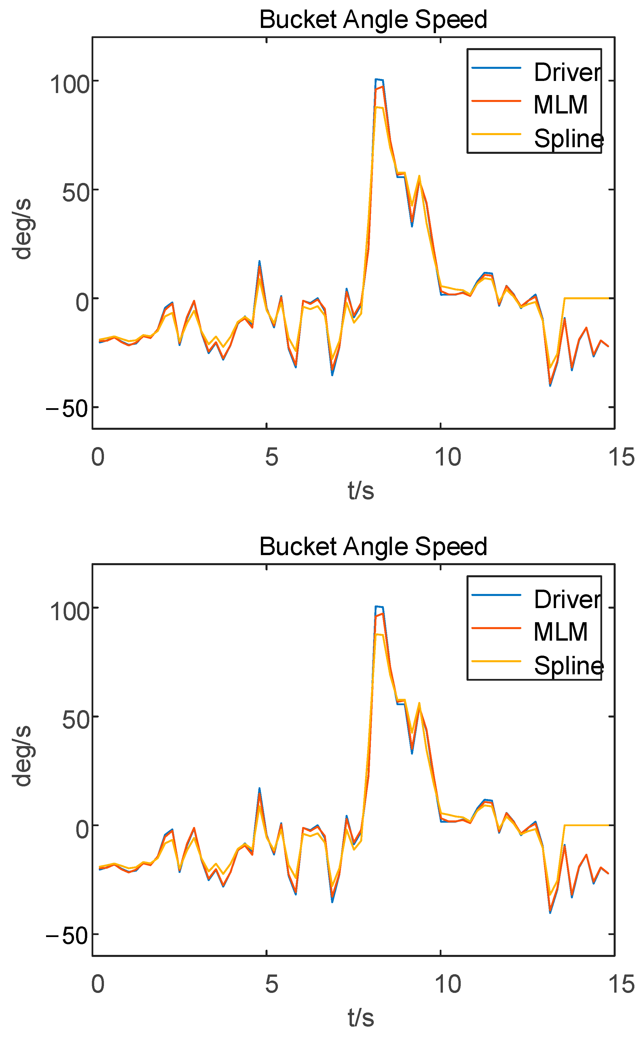
The speed comparison between the operator-operated trajectory, the machine learning model-generated trajectory, and the spline curve model-generated trajectory is illustrated in the subsequent figure (Figure 12).
Based on the aforementioned comparison, it is evident that all three models exhibit a consistent trend in terms of changes in their movement speeds. In contrast to the operator-controlled trajectories, both the machine learning model and the spline curve model demonstrate a decrease in the maximum speed; however, the machine learning model experiences a more pronounced decline. This suggests that the control system enables target trajectory tracking for the machine learning model with reduced energy consumption, thereby highlighting its superiority over the control system (Table 5).
Based on the table presented above, it can be inferred that the mining trajectory generated by the machine learning model demonstrates a decrease in the maximum angular velocities of the boom, arm, bucket, and swing joint by 8.64 deg/s, 10.24 deg/s, 18.33 deg/s, and 1.6 deg/s, respectively. This outcome surpasses that of the spline curve model.
When employing conventional approaches for trajectory generation, it is imperative to meticulously examine and formulate appropriate rules for trajectory planning. The computational resources required for trajectory generation calculations are generally minimal and do not necessitate a machine learning training phase. Hence, it becomes essential to compare the cost of machine learning with traditional trajectory generation methods. We generated 3100 planned trajectories on the same computer and conducted a comparative analysis between the two methods in terms of memory usage, computation time, and training time to assess their computational costs. The traditional method utilized MATLAB tools for generating the trajectories. The specific outcomes are presented in the table below (Table 6).
After conducting a thorough comparison, it was observed that traditional methods exhibit advantages in terms of memory utilization and training duration. However, when it comes to generating a substantial number of trajectories, their computational time experiences a significant prolongation. Conversely, machine learning models demonstrate an evident superiority in generating an extensive volume of trajectories, thereby implying acceptable levels of memory usage and training time.
4. Conclusions
After collecting data from professional operators conducting high-platform excavation operations with excavators, we constructed a preliminary sample of operator operation curves and expanded the sample using bootstrap resampling techniques. Key features were extracted as the inputs, and machine learning methods were employed to train the samples. Consequently, we successfully established an excavation trajectory generation model and validated it as an exceptional method for generating trajectories. By comparing the trajectories generated by the machine learning model with those produced by spline curve models and the actual operator trajectories in terms of angles and angular velocities, we observed that the accuracy of the machine learning-generated trajectories significantly surpassed that of the spline curve models. Furthermore, when examining speed variations among the machine learning model trajectories, operator trajectories, and spline curve trajectories, our findings revealed that the speed changes generated by the machine learning model were smoother and exhibited superior adaptability within the control systems. In the future, we will further investigate two aspects. Firstly, we aim to eliminate the need for manually specifying key points in the trajectory and instead analyze professional operators’ operational trajectories directly using deep learning methods. This approach aims to establish a trajectory planning method that is independent of subjective factors introduced by researchers, thereby forming a rule-free trajectory planning approach. Secondly, we will conduct machine learning research on additional working conditions based on professional operators’ data and develop machine learning-based trajectory planning methods for the automatic recognition and extraction of typical working conditions such as excavation, ground leveling, slope repair, and trenching.
Author Contributions
Methodology, Z.J., M.G. and J.L.; Software, S.L.; Validation, G.L.; Formal analysis, Z.J.; Resources, D.Z.; Data curation, Z.J.; Writing—original draft, Z.J.; Writing—review & editing, Y.Z. and W.L.; Supervision, M.G. All authors have read and agreed to the published version of the manuscript.
Funding
This work was supported by the Natural Science Foundation of Hebei Province, China, under Grant No. E2021203145, the National Natural Science Foundation of China under Grant No. 52175063 for the research on active vibration control theory and vehicle attitude control strategy of emergency rescue vehicles with active suspension systems, and the Joint Fund for Regional Innovation Development of National Natural Science Foundation of China under Grant No. U20A20332 for the study on the dynamic control of highly maneuverable emergency rescue vehicles based on multi-information fusion. This work was supported in part by the Special Carrier Equipment Research Center of Yanshan University.
Data Availability Statement
Data are contained within this article.
Acknowledgments
The authors would like to express their thanks to the Natural Science Foundation of Hebei Province, China.
Conflicts of Interest
Authors Zhong Jin, Shaomeng Luo, Guowang Li and Jiaheng Li were employed by the company Guangxi Liugong Machinery Co., Ltd. The remaining authors declare that the research was conducted in the absence of any commercial or financial relationships that could be construed as a potential conflict of interest. The [company Guangxi Liugong Machinery Co., Ltd.-companies in affiliation and funding] had no role in the design of the study; in the collection, analyses, or interpretation of data; in the writing of the manuscript, or in the decision to publish the results.
References
- Yoo, S.; Park, C.G.; You, S.H. A Dynamics-Based Optimal Trajectory Generation for Controlling an Automated Excavator. Proc. Inst. Mech. Eng. Part C J. Mech. Eng. Sci. 2010, 224, 2109–2119. [Google Scholar] [CrossRef]
- Zou, Z.; Chen, J.; Pang, X. Task space-based dynamic trajectory planning for digging process of a hydraulic excavator with the integration of soil–bucket interaction. Proc. Inst. Mech. Eng. Part K J. Multi-Body Dyn. 2019, 233, 598–616. [Google Scholar] [CrossRef]
- Jud, D.; Hottiger, G.; Leemann, P.; Hutter, M. Planning and Control for Autonomous Excavation. IEEE Robot. Autom. Lett. 2017, 2, 2151–2158. [Google Scholar] [CrossRef]
- Jud, D.; Leemann, P.; Kerscher, S.; Hutter, M. Autonomous Free-Form Trenching Using a Walking Excavator. IEEE Robot. Autom. Lett. 2019, 4, 3208–3215. [Google Scholar] [CrossRef]
- Kim, Y.B.; Ha, J.; Kang, H.; Kim, P.Y.; Park, J.; Park, F. Dynamically optimal trajectories for earthmoving excavators. Autom. Constr. 2013, 35, 568–578. [Google Scholar] [CrossRef]
- Groll, T.; Hemer, S.; Ropertz, T.; Berns, K. Autonomous trenching with hierarchically organized primitives. Autom. Constr. 2019, 98, 214–224. [Google Scholar] [CrossRef]
- Lee, D.; Jang, I.; Byun, J.; Seo, H.; Kim, H.J. Real-Time Motion Planning of a Hydraulic Excavator using Trajectory Optimization and Model Predictive Control. arXiv 2021. [Google Scholar] [CrossRef]
- Zhang, Y.; Sun, Z.; Sun, Q.; Wang, Y.; Li, X.; Yang, J. Time-jerk optimal trajectory planning of hydraulic robotic excavator. Adv. Mech. Eng. 2021, 13, 168781402110346. [Google Scholar] [CrossRef]
- Zhao, J.; Zhang, L. TaskNet: A Neural Task Planner for Autonomous Excavator. In Proceedings of the 2021 IEEE International Conference on Robotics and Automation (ICRA), Xi’an, China, 30 May–5 June 2021; pp. 2220–2226. [Google Scholar] [CrossRef]
- Feng, H.; Jiang, J.; Ding, N.; Shen, F.; Yin, C.; Cao, D.; Li, C.; Liu, T.; Xie, J. Multi-objective time-energy-impact optimization for robotic excavator trajectory planning. Autom. Constr. 2023, 156, 105094. [Google Scholar] [CrossRef]
- Park, J.; Lee, B.; Kang, S.; Kim, P.Y.; Kim, H.J. Online Learning Control of Hydraulic Excavators Based on Echo-State Networks. IEEE Trans. Autom. Sci. Eng. 2017, 14, 249–259. [Google Scholar] [CrossRef]
- Zhou, Q.; Chen, G.; Jiang, W.; Li, K.; Li, K. Automatically Detecting Excavator Anomalies Based on Machine Learning. Symmetry 2019, 11, 957. [Google Scholar] [CrossRef]
- Oguma, S.; Omatsu, S.; Ohno, S.; Iwasaki, K.; Shishido, Y. Failure Prediction Based on Operational Data of Hydraulic Excavator with Machine Learning. IEEJ Trans. Electr. Electron. Eng. 2021, 16, 1438–1440. [Google Scholar] [CrossRef]
- Seker, S.E.; Ibrahim, O. Performance Prediction of Roadheaders Using Ensemble Machine Learning Techniques. Neural Comput. Appl. 2019, 31, 1103–1116. [Google Scholar] [CrossRef]
- Kurinov, I.; Orzechowski, G.; Hamalainen, P.; Mikkola, A. Automated Excavator Based on Reinforcement Learning and Multibody System Dynamics. IEEE Access 2020, 8, 213998–214006. [Google Scholar] [CrossRef]
- Samtani, P.; Leiva, F.; Ruiz-Del-Solar, J. Learning to Break Rocks With Deep Reinforcement Learning. IEEE Robot. Autom. Lett. 2023, 8, 1077–1084. [Google Scholar] [CrossRef]
- Lee, M.; Choi, H.; Kim, C.; Moon, J.; Kim, D.; Lee, D. Precision Motion Control of Robotized Industrial Hydraulic Excavators via Data-Driven Model Inversion. IEEE Robot. Autom. Lett. 2022, 7, 1912–1919. [Google Scholar] [CrossRef]
- Egli, P.; Gaschen, D.; Kerscher, S.; Jud, D.; Hutter, M. Soil-Adaptive Excavation Using Reinforcement Learning. IEEE Robot. Autom. Lett. 2022, 7, 9778–9785. [Google Scholar] [CrossRef]
- Yu, S.; Song, X.; Sun, Z. On-Line Prediction of Resistant Force During Soil–Tool Interaction. Dyn. Syst. Meas. Control. 2023, 145, 081004. [Google Scholar] [CrossRef]
- Li, S.; Wang, S.; Chen, X.; Zhou, G.; Wu, B.; Hou, L. Application of Physics-Informed Machine Learning for Excavator Working Resistance Modeling. Mech. Syst. Signal Process. 2024, 209, 111117. [Google Scholar] [CrossRef]
- Guo, Q.; Ye, Z.; Wang, L.; Zhang, L. Imitation Learning and Model Integrated Excavator Trajectory Planning. In Proceedings of the 2022 IEEE RSJ International Conference on Intelligent Robots and Systems (IROS), Kyoto, Japan, 23–27 October 2022; pp. 5737–5743. [Google Scholar] [CrossRef]
- Osa, T.; Aizawa, M. Deep Reinforcement Learning With Adversarial Training for Automated Excavation Using Depth Images. IEEE Access 2022, 10, 4523–4535. [Google Scholar] [CrossRef]
- Kim, J.; Seokho, C. Action Recognition of Earthmoving Excavators Based on Sequential Pattern Analysis of Visual Features and Operation Cycles. Autom. Constr. 2019, 104, 255–264. [Google Scholar] [CrossRef]
- Yao, Z.; Zhao, S.; Tan, X.; Wei, W.; Wang, Y. Real-time task-oriented continuous digging trajectory planning for excavator arms. Autom. Constr. 2023, 152, 104916. [Google Scholar] [CrossRef]
- Zhao, J.; Tan, P.; Hu, Y.; Tian, M.; Xia, X. Autonomous Excavation Trajectory Generation for Trenching Tasks Based on Skills of Skillful Operator. In Proceedings of the 2022 International Conference on Mechanical and Electronics Engineering (ICMEE), Xi’an, China, 21–23 November 2022; pp. 134–138. [Google Scholar] [CrossRef]
- Yang, Y.; Zhang, L.; Cheng, X.; Pan, J.; Yang, R. Compact Reachability Map for Excavator Motion Planning. In Proceedings of the 2019 IEEE/RSJ International Conference on Intelligent Robots and Systems (IROS), Macau, China, 3–8 November 2019; IEEE: Macau, China, 2019; pp. 2308–2313. [Google Scholar] [CrossRef]
- Tremblay, L.F.Y.; Arsenault, M.; Zeinali, M. Development of a trajectory planning algorithm for a 4-DoF rockbreaker based on hydraulic flow rate limits. Trans. Can. Soc. Mech. Eng. 2020, 44, 501–510. [Google Scholar] [CrossRef]
- Picheny, V.; Kim, N.H.; Haftka, R.T. Application of bootstrap method in conservative estimation of reliability with limited samples. Struct. Multidiscip. Optim. 2010, 41, 205–217. [Google Scholar] [CrossRef]
- Yang, Y.; Long, P.; Song, X.; Pan, J.; Zhang, L. Optimization-Based Framework for Excavation Trajectory Generation. IEEE Robot. Autom. Lett. 2021, 6, 1479–1486. [Google Scholar] [CrossRef]
- Zhang, B.; Wang, S.; Liu, Y.; Yang, H. Research on Trajectory Planning and Autodig of Hydraulic Excavator. Math. Probl. Eng. 2017, 2017, 7139858. [Google Scholar] [CrossRef]
- Yang, J.; Gao, Y.; Guo, R.; Gao, Q.; Zhao, J. Research on Excavator Trajectory Control Based on Hybrid Interpolation. Sustainability 2023, 15, 6761. [Google Scholar] [CrossRef]
- Ding, H.; Sang, Z.; Li, Z.; Shi, J.; Wang, Y.; Meng, D. Trajectory planning and control of large robotic excavators based on inclination-displacement mapping. Autom. Constr. 2024, 158, 105209. [Google Scholar] [CrossRef]
- Huh, J.; Bae, J.; Lee, D.; Kwak, J.; Moon, C.; Im, C.; Ko, Y.; Kang, T.K.; Hong, D. Deep Learning-Based Autonomous Excavation: A Bucket-Trajectory Planning Algorithm. IEEE Access 2023, 11, 38047–38060. [Google Scholar] [CrossRef]
- Egli, P.; Marco, H. A General Approach for the Automation of Hydraulic Excavator Arms Using Reinforcement Learning. IEEE Robot. Autom. Lett. 2022, 7, 5679–5686. [Google Scholar] [CrossRef]
Figure 1.
Professional operator job scenario illustration.

Figure 2.
Post-expansion job cycle samples and joint angle amplitude samples.


Figure 3.
Four expanded joint trajectory curves (The colors of the 3100 lines were randomly assigned).
Figure 3.
Four expanded joint trajectory curves (The colors of the 3100 lines were randomly assigned).


Figure 4.
Definition of excavator coordinate system.

Figure 5.
Proficient operator maneuvering curve contours.

Figure 6.
Diagram of six key point positions.


Figure 7.
The key point lies in the position diagram of joint trajectories.

Figure 8.
Machine learning for mining trajectory generation.

Figure 9.
Machine learning loss function curve.

Figure 10.
3100 trajectory curves generated by machine learning models (The colors of the 3100 lines were randomly assigned).
Figure 10.
3100 trajectory curves generated by machine learning models (The colors of the 3100 lines were randomly assigned).


Figure 11.
Comparison between operator trajectory, spline curve model trajectory, and machine learning model trajectory.
Figure 11.
Comparison between operator trajectory, spline curve model trajectory, and machine learning model trajectory.


Figure 12.
Comparison of angular velocities between manual operation trajectory, spline curve model trajectory, and machine learning model trajectory.
Figure 12.
Comparison of angular velocities between manual operation trajectory, spline curve model trajectory, and machine learning model trajectory.


Table 1.
Relevant parameters of excavator joints.
| θmin (deg) | θmax/deg | θrange/deg | Note | |
|---|---|---|---|---|
| Rotating | 0 | 360 | 360 | Rotate continuously |
| Boom | −48 | 65 | 113 | Relative to the water level |
| Arm | −158 | −35 | 123 | Relative to boom |
| Bucket | −150 | 49 | 199 | Relative to arm |
Table 2.
Machine learning model input, model label, and model output.
| Symbol | Variable | Description | Unit | |
|---|---|---|---|---|
| Model Input | x1~x6 | Time of key point | s | |
| x7~x12 | Angle values of the pivotal boom | deg | ||
| x13~x18 | Angle values of the pivotal arm | deg | ||
| x19~x24 | Angle values of the pivotal bucket | deg | ||
| x25~x30 | Angle values of the pivotal swing | deg | ||
| Model Label | y1~y72 | Time of the operator curve | s | |
| y73~y144 | Boom angle of the operator curve | deg | ||
| y145~y216 | Arm angle of the operator curve | deg | ||
| y217~y288 | Bucket angle of the operator curve | deg | ||
| y289~y360 | Swing angle of the operator curve | deg | ||
| Model Output | Time of the deep learn model | s | ||
| Boom angle of the deep learn model | deg | |||
| Arm angle of the deep learn model | deg | |||
| Bucket angle of the deep learn model | deg | |||
| Swing angle of the deep learn model | deg |
Table 3.
Comparison of neural network models with different parameters.
| No. | Network Layers | Number of Neurons Per Layer | Parameter Quantity | Training Parameters |
|---|---|---|---|---|
| 1 | 5 | 256 | 297,832 | Training epochs: 15,000 Optimizer: Adam Learning rate: 0.001 Learning rate strategy: Exponential decay Loss function adjustment: Mean squared error |
| 2 | 10 | 256 | 626,792 | |
| 3 | 15 | 256 | 955,752 | |
| 4 | 5 | 512 | 988,520 | |
| 5 | 10 | 512 | 2,301,800 | |
| 6 | 15 | 512 | 3,615,080 |
Table 4.
The maximum deviation of the joint angles between the spline curve model and the machine learning model.
Table 4.
The maximum deviation of the joint angles between the spline curve model and the machine learning model.
| θboom/deg | θarm/deg | θbucket/deg | θswing/deg | |
|---|---|---|---|---|
| Spline curve model | 4.22 | 4.97 | −3.2 | −4.98 |
| Machine learning model | 1.74 | −2.99 | −2.4 | −2.6 |
Table 5.
Comparison of maximum angular velocities for three trajectories.
| ωmax boom deg/s | ωmax arm deg/s | ωmax bucket deg/s | ωmax swing deg/s | |
|---|---|---|---|---|
| Operator’s trajectory | −33.89 | 47.58 | 90.58 | −41.38 |
| Spline curve model | −23.51 | 39.80 | 90.23 | −43.27 |
| Machine learning model | −25.25 | 37.34 | 72.25 | −39.78 |
Table 6.
Comparison of costs between traditional methods and ML models.
| Memory Usage | Computation Time | Training Time | |
|---|---|---|---|
| Spline curve model | 768 Kb | 1.5 s | 0 s |
| Machine learning model | 1014 Kb | 0.14 s | 0.231 s |
Disclaimer/Publisher’s Note: The statements, opinions and data contained in all publications are solely those of the individual author(s) and contributor(s) and not of MDPI and/or the editor(s). MDPI and/or the editor(s) disclaim responsibility for any injury to people or property resulting from any ideas, methods, instructions or products referred to in the content. |
© 2024 by the authors. Licensee MDPI, Basel, Switzerland. This article is an open access article distributed under the terms and conditions of the Creative Commons Attribution (CC BY) license (https://creativecommons.org/licenses/by/4.0/).
Share and Cite
MDPI and ACS Style
Jin, Z.; Gong, M.; Zhao, D.; Luo, S.; Li, G.; Li, J.; Zhang, Y.; Liu, W. Mining Trajectory Planning of Unmanned Excavator Based on Machine Learning. Mathematics 2024, 12, 1298. https://0-doi-org.brum.beds.ac.uk/10.3390/math12091298
AMA Style
Jin Z, Gong M, Zhao D, Luo S, Li G, Li J, Zhang Y, Liu W. Mining Trajectory Planning of Unmanned Excavator Based on Machine Learning. Mathematics. 2024; 12(9):1298. https://0-doi-org.brum.beds.ac.uk/10.3390/math12091298
Chicago/Turabian StyleJin, Zhong, Mingde Gong, Dingxuan Zhao, Shaomeng Luo, Guowang Li, Jiaheng Li, Yue Zhang, and Wenbin Liu. 2024. "Mining Trajectory Planning of Unmanned Excavator Based on Machine Learning" Mathematics 12, no. 9: 1298. https://0-doi-org.brum.beds.ac.uk/10.3390/math12091298
Note that from the first issue of 2016, this journal uses article numbers instead of page numbers. See further details here.