A p-Refinement Method Based on a Library of Transition Elements for 3D Finite Element Applications

Abstract

Wave propagation or acoustic emission waves caused by impact load can be simulated using the finite element (FE) method with a refined high-fidelity mesh near the impact location. This paper presents a method to refine a 3D finite element mesh by increasing the polynomial order near the impact location. Transition elements are required for such a refinement operation. Three protocols are defined to implement the transition elements within the low-order FE mesh. Due to the difficulty of formulating shape functions and verification, there are no transition elements beyond order two in the current literature for 3D elements. This paper develops a complete set of transition elements that facilitate the transition from first- to fourth-order Lagrangian elements, which facilitates mesh refinement following the protocols. The shape functions are computed and verified, and the interelement compatibility conditions are checked for each element case. The integration quadratures and shape function derivative matrices are also computed and made readily available for FE users. Finally, two examples are presented to illustrate the applicability of this method.

1. Introduction

Interest in space activities, including satellite launches, space tourism, deep-space exploration, and space colonization, has increased in recent years. The development of long-term deep-space habitats is of interest to the engineering community. These structures will be exposed to harsh environmental loading conditions, including hypervelocity impact (HVI) caused by meteoroids or debris. The finite element method (FEM) is a widely used numerical approach for solving partial differential equations (PDEs) in mathematics and engineering, especially in the field of structural dynamics [1,2,3]. However, the solutions of wave propagation problems cannot be effectively replicated through a standard FEM. In the case of harmonic wave solutions, it is well known that the accuracy of numerical solutions rapidly degrades as the wave number increases [4,5]. Novel techniques based on higher-order discontinuous Galerkin methods exist to mitigate this issue [6,7]. In the field of FEM, there are two methods of reducing error and improving the ability of the basis functions to represent the variation of the unknown function over the local domain: (1) increasing the number of the elements, or h-refinement, and (2) increasing the polynomial order, or p-refinement. H-refinement techniques have been used widely in conjunction with low-order vector basis functions. However, very fine meshes are necessary to find reasonable solutions for problems with short waves—so fine that the numerical solution effort may be prohibitive. The spectral element approach offers a great solution for resolving this issue [8,9,10,11,12]. In this case, high-order Lagrangian-based finite elements are employed in conjunction with particular nodal positions and integration algorithms. In comparison to typical finite element methods, this method has low numerical dispersion and can be particularly effective in explicit time integration. While implementing a high-order element in a lower-order mesh, p-refinement is needed [13]. However, due to the relatively recent emergence of higher-order hierarchical vector basis functions, p-refinement approaches have not been widely researched to date [14,15,16].

The advantage of p-refinement is that it eliminates the time-consuming mesh regeneration procedure associated with h-refinement. The process must be adaptable to benefit fully from either type of refinement technique. Adaptive refinement uses the error estimate from a numerical solution at a particular level of refinement to forecast which areas of the computational domain will most require more degrees of freedom. After that, the process remedies the issue by allocating more degrees within certain zones. Since they enable most of the equations in the FEM system to stay constant across refinement levels, hierarchical vector basis functions are virtually always used for adaptive refinement. Conversely, interpolatory vector basis functions would necessitate the replacement of all equations in the regions that are being refined. Furthermore, unique transition elements are needed in an interpolatory expansion in order to link regions with varying polynomial degrees [14].

In a three-dimensional finite element application, hexahedron transition elements are extensively used for p-mesh refinement [17]. When implementing a transition element in a multi-element mesh, the hanging node problem arises. This violates the interelement compatibility conditions. Hence, several strategies to circumvent the hanging node problem have been developed. For two-dimensional applications, variable-node elements for 1-irregular/balanced meshes have been constructed by Gupta, while Morton et al. published an extension for three dimensions [18]. These elements utilize piecewise linear shape functions on their boundaries, so two smaller finite elements can be coupled conformally to a larger transition element [1]. Gordon and co-workers developed a transfinite interpolation or blending function method [19], where the functions are identical in certain parts but not over the whole domain [20]. Scholz developed two- and three-dimensional transition elements with piecewise linear and quadratic shape functions for mesh refinement purposes [21], where 1-irregular meshes can be generated without introducing hanging nodes. Developing higher-order transition elements is a challenge. Unconventional elements, such as the xNy-element concept [14,16], are developed by utilizing linear blending functions and projection operators to tackle this issue. However, there is still the problem of efficient mesh generation for these transition elements, especially for three-dimensional models, as this procedure is very cumbersome [22].

Transition elements are also employed in contact problems [23]. Buczkowski [24] developed 22- and 21-node elements, and Smith et al. [25] developed 14-node hexahedral isoparametric elements to analyze contact problems by modifying the reference 8- and 20-node hexahedral elements. The modification of the shape functions of the reference element needs to be carried out by hand and is very laborious for a 3D element. In addition to lower-order transition elements, there is also a need for higher-order transition elements, as they offer higher accuracy when calculating Lagrangian solid dynamics. For instance, the spectral finite element method [9] uses the interpolation function of high-order Lagrange polynomials to capture high-frequency wave propagation that benefits fields such as structural health monitoring [10,11,12,26] and seismology [8]. Employing transition elements can reduce the degrees of freedom and computation effort for such applications.

A library of transition elements can mitigate these issues. However, creating a library is very labor-intensive when higher-order elements are considered. The shape functions of higher-order elements are numerous and lengthy, so it is extremely difficult to modify and verify them to form a higher-order transition element. In summary, there is no methodology for formulating arbitrary hexahedron elements and implementing multi-element mesh that is programmatically available. Hence, there is no transition element beyond order 2 in the literature.

This paper develops a method to perform p-refinement that involves three protocols. The implementation of these protocols is based on a library of transition elements. Six 3D transition elements of an order up to four are developed to act as a library that can facilitate the p-refinement procedure. The development procedure utilizes the GUI developed in [16]. First, the reference element, the Lagrangian [27] or Serendipity [28] element that represents a transition element closely in terms of element order, is formulated following methods available in the literature. The formulation includes the nodal coordinates and the monomial basis functions of the interpolation function. Next, the generated nodal coordinates and the monomial basis functions are modified to replicate the transition element. The nodal coordinates and interpolation function consist of the monomial basis functions that will be used to formulate the shape functions. The modification of the monomial basis functions is extremely simple compared to the modification of the shape functions. However, the method for determining the shape functions is very laborious and can be carried out by hand for one-dimensional and lower-order two-dimensional elements [29]. For this reason, the computer algorithm was implemented to automate this task instead [16]. Finally, the element is verified in terms of local support and interelement compatibility conditions [29].

The remainder of this paper is organized as follows: Section 2 presents the methodology for p-refinement and generating element properties, while Section 3 showcases the implementation and results for the formulated transition elements. The developed p-refinement method is verified for an FE mesh that contains all six transition elements developed in this paper through a patch test [30]. Subsequently, this method is implemented in two 3D FE meshes and, finally, Section 4 concludes this paper with some final remarks.

2. Materials and Methods

In this section, a procedure is developed to perform p-refinement for the given refined element. First, the protocol to refine a single element is presented. Then the method based on the protocol to refine all the elements in the mesh is illustrated.

2.1. p-Refinement Procedure

Assume that element $e_i$ is refined as order $n$, and another adjacent element, $e_j$, needs to be refined so that it can (1) act as a transition element from order $n$ to order $n-1$, and (2) satisfy the interelement boundary conditions. Due to this dependency of element $e_j$ on $e_i$, the elements $e_i$ and $e_j$ are termed as master and slave elements, respectively. Three protocols have been developed to refine element $e_j$, shown as a linear eight-node brick element, with node numbers ranging from 1 to 8 at the local coordinate [2].

Protocol 1: Only one edge has the highest order. Assume element $e_i$ shares an edge with element $e_j$, where the order of the edge is $n$, as presented in Figure 1. In this case, the transition element will have order $n$ only at the edge and order $n-1$ everywhere else. This paper defines the edge by nodes 7–8 in local coordinates.

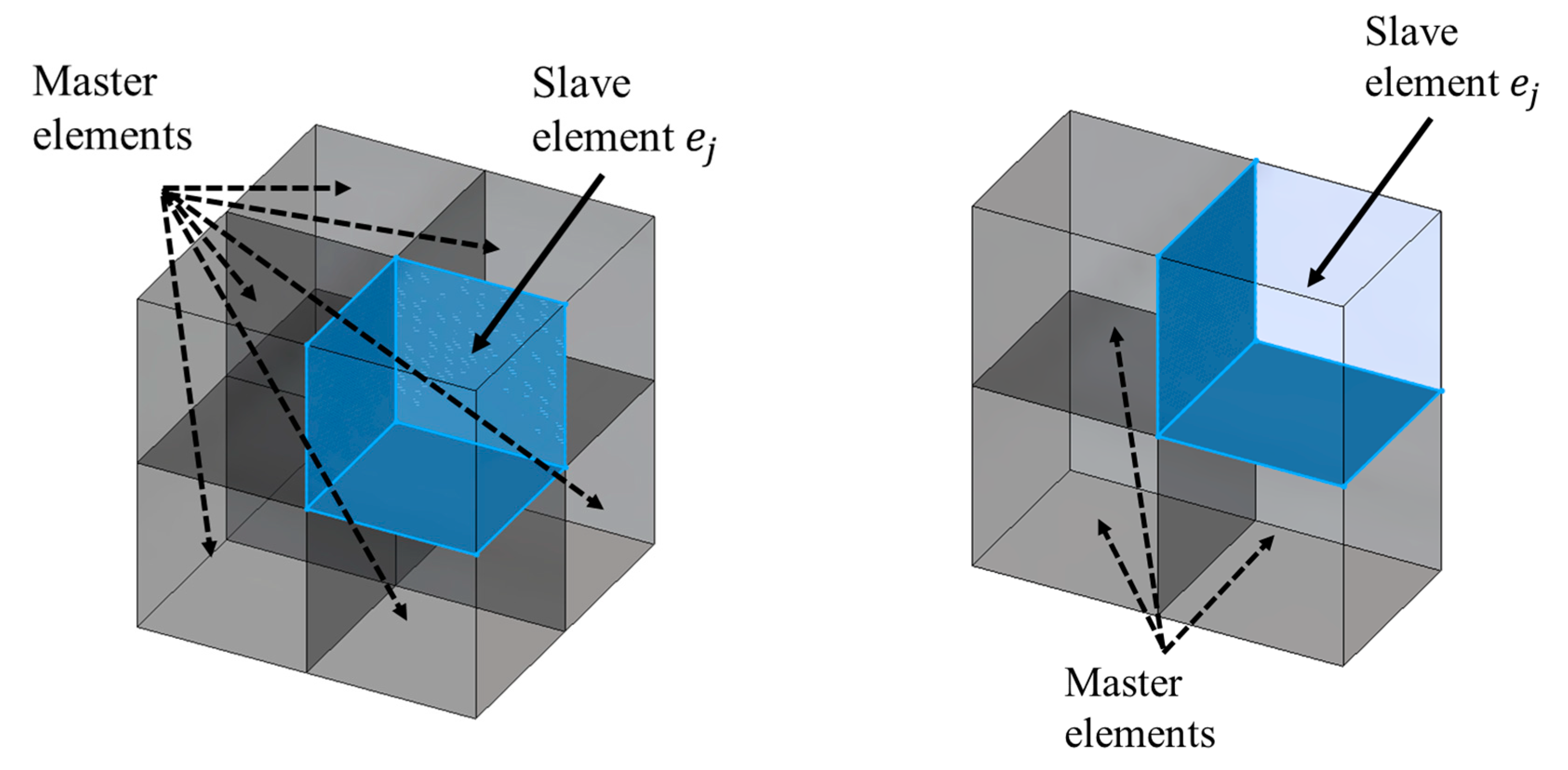
Protocol 2: Four edges have the highest order, and that forms the face of the element. If four edges form an interelement surface, the order at the surface will be $n$ and $n-1$ everywhere else. A schematic of this case is presented in Figure 2, where the nodes 5–8 define the interelement surface.

Protocol 3: More than four edges have order $n$. For protocol 3, there will be several master elements that form an interelement boundary with the element to be refined ($e_j$). If there are more than four edges, the order will be $n$ throughout the element space. Two cases with more than four edges at the interface are presented in Figure 3, where the dark elements are of order $n$; hence, the order of the element $e_j$ will be $n$.

The p-refinement utilizes one transition element for each protocol that follows the node number presented above. The formulation of these elements is presented in the next subsection. The shared boundary between elements $e_j$ and $e_j$ does not necessarily match the node numbering sequence (7–8 for protocol 1) in local coordinates. Hence, while implementing the transition elements, the node number of element $e_j$ needs to be renamed to match the transition element with no number. The refinement is followed by the refinement of element $e_j$, carried out element by element from the lowest to the highest distance from the element centroids with respect to $e_i$. The transition of element order decreases by one as the refinement continues. For 8-noded elements, the distance follows

$$d_{ij}=‖{\left(\frac{\sum _{k=1}^8\left[\begin{array}{ccc}{x}_k& y_k& z_k\end{array}\right]}{8}\right)}_{e_i}-{\left(\frac{\sum _{k=1}^8\left[\begin{array}{ccc}{x}_k& y_k& z_k\end{array}\right]}{8}\right)}_{e_j}‖$$

(1)

where $\left[\begin{array}{ccc}{x}_i& y_i& z_i\end{array}\right]$ is the nodal coordinate of node $i$ and $‖.‖$ indicates the second norm. A 2D overview is presented for a four-element case in Figure 4, where $d_{ij}<d_{il}<d_{ik}$. Hence, the refinement procedure is carried out on element $j$ first, then element $l,$ and finally $k$. The refinement for the whole mesh involves:

1.

Creating a set of $d_{ij}$ following Equation (1), and sorting from lowest to the highest;

2.

For each element associated with the sorted $d_{ij}$, $e_j$:

• determining all the adjacent elements for $e_j$;
• For each adjacent element, obtaining the interelement boundary order;
• If the order of the element boundary > the order of $e_j$:
  • Renaming the node number of $e_j$ to match the interelement boundary;
  • Refining the element following the protocol.

2.2. Formulation of Transition Elements

This section illustrates the procedure to formulate and implement a transition element within a multi-element FE mesh, as presented in Figure 5. First, the nodal coordinates and the monomial basis function of the reference element are computed. The reference element is the element that closely resembles the arbitrary element in terms of element order and type (Lagrangian or Serendipity).

Next, the nodal coordinates and the monomial basis functions are updated to replicate the arbitrary element. The shape functions for these two inputs are then determined through computer implementation [3]. If the shape functions can be determined, verification of the local support conditions will be carried out. Next, the element can be incorporated into a multi-element mesh if the interelement compatibility is satisfied between the adjacent elements of different types. If the element is compatible, the formulation is complete and ready to be implemented for FE applications.

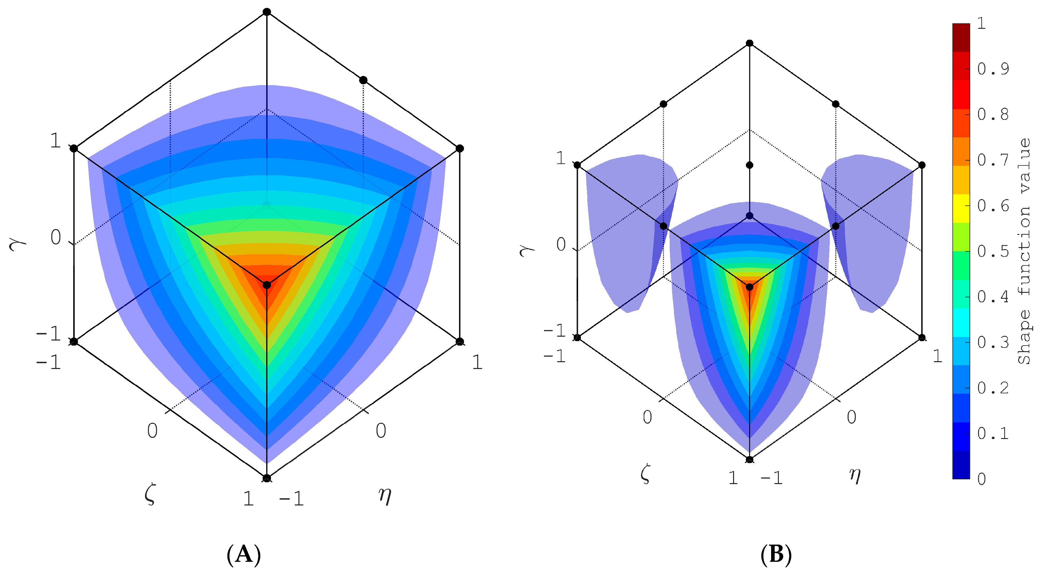
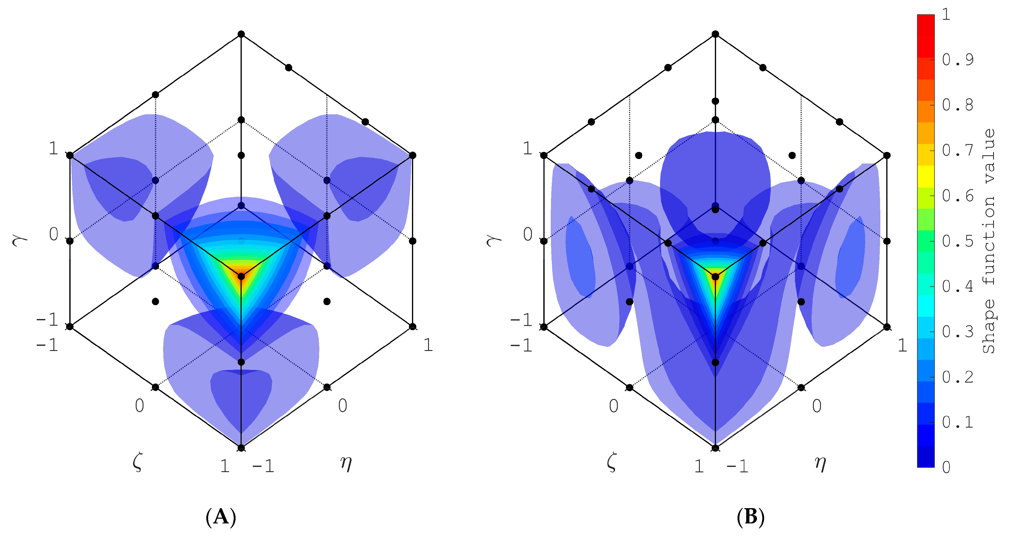
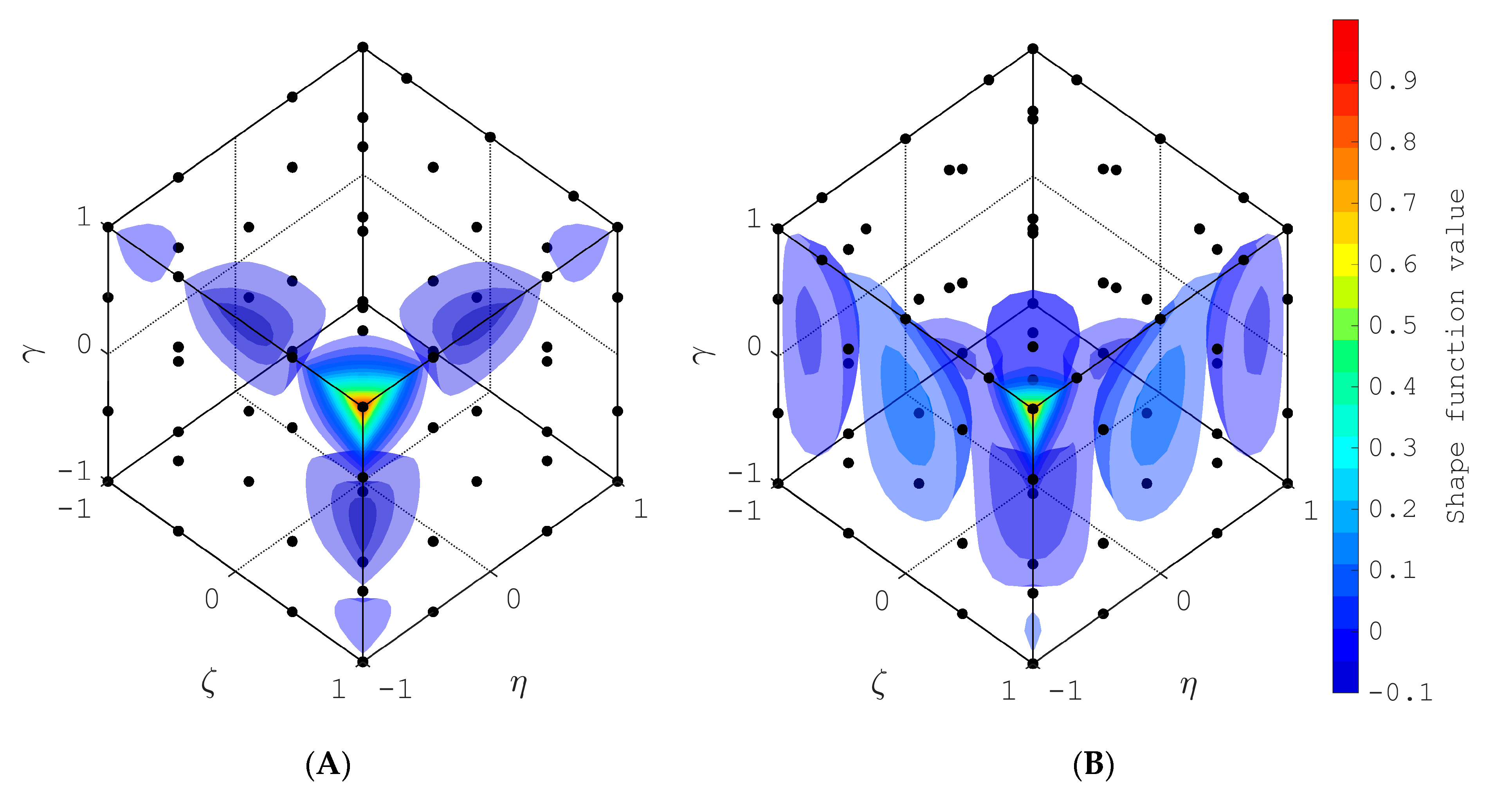
For this purpose, methodology and the toolbox, ShapeGen3D v.1, developed by [16] is utilized. Here, the element is subdivided into a 3D grid, and the value of the shape functions is determined for each point. The results are plotted, with the void where the value of the shape function is 0. Hence, if a surface does not contain a node $i$, and there is a void throughout for the value of shape function $i$, the element satisfies the local support condition for that shape function. The interelement compatibility conditions are also checked and satisfied following the procedure described in [16]. In addition to the shape function value, the integration points and weights for the Gauss–Lobatto [27] quadrature was obtained.

3. Results

3.1. Transition Elements

Six transition elements that enable the transition from the fourth- to first-order Lagrangian element were formulated. All the elements underwent an interelement compatibility check to make sure they could form a multi-element mesh. A second-to-first-order transition element for case 2 is presented in detail in Figure 6. Figure 6A shows the two elements assembled to form an interelement boundary. The red hollow diamond represents the nodes of the second order, whereas the black dots represent the nodes of the transition element. The interelement boundary is presented in Figure 6B, which shows that the nodes coincide and shape function profiles corresponding to the node of these two elements match each other. As all the shape functions corresponding to the common nodes matched, the $\zeta$ = 1 surface of the transition element was compatible with the second-order element.

The parameters obtained for each of the elements are

• Nodal coordinates;
• Shape functions;
• Integration quadrature.

The parameters obtained for these transition elements are lengthy and difficult to describe in a paper. Hence, only the results for the transition element presented in Figure 6 are detailed in Appendix A.

Table A1. Node coordinates of the 13-node transition element.

Node No.	x	y	z
1	−1	−1	−1
2	1	−1	−1
3	1	1	−1
4	1	−1	−1
5	−1	−1	1
6	1	−1	1
7	1	1	1
8	1	−1	1
9	0	−1	1
10	1	0	1
11	0	1	1
12	−1	0	1
13	0	0	1

,

Table A2. Shape functions of the 13-node transition element.

${\mathit{N}}_{\mathit{i}}$	$\mathbf{Shape} \mathbf{Functions} \mathbf{in} \mathbf{Terms} \mathbf{of} (\mathit{x},\mathit{y},\mathit{z})$
$N_1$	$\frac{xy}{8}-\frac{y}{8}-\frac{z}{8}-\frac{x}{8}+\frac{xz}{8}+\frac{yz}{8}-\frac{xyz}{8}+\frac{1}{8}$
$N_2$	$\frac{x}{8}-\frac{y}{8}-\frac{z}{8}-\frac{xy}{8}-\frac{xz}{8}+\frac{yz}{8}+\frac{xyz}{8}+\frac{1}{8}$
$N_3$	$\frac{x}{8}+\frac{y}{8}-\frac{z}{8}+\frac{xy}{8}-\frac{xz}{8}-\frac{yz}{8}-\frac{xyz}{8}+\frac{1}{8}$
$N_4$	$\frac{y}{8}-\frac{x}{8}-\frac{z}{8}-\frac{xy}{8}+\frac{xz}{8}-\frac{yz}{8}+\frac{xyz}{8}+\frac{1}{8}$
$N_5$	$\frac{xy}{8}-\frac{x{y}^2\left(z+1\right)}{8}-\frac{x^{2}y\left(z+1\right)}{8}+\frac{xyz}{8}+\frac{x^2{y}^2\left(z+1\right)}{8}$
$N_6$	$\frac{x{y}^2\left(z+1\right)}{8}-\frac{xy}{8}-\frac{x^{2}y\left(z+1\right)}{8}-\frac{xyz}{8}+\frac{x^2{y}^2\left(z+1\right)}{8}$
$N_7$	$\frac{xy}{8}+\frac{x{y}^2\left(z+1\right)}{8}+\frac{x^{2}y\left(z+1\right)}{8}+\frac{xyz}{8}+\frac{x^2{y}^2\left(z+1\right)}{8}$
$N_8$	$\frac{x^{2}y\left(z+1\right)}{8}-\frac{x{y}^2\left(z+1\right)}{8}-\frac{xy}{8}-\frac{xyz}{8}+\frac{x^2{y}^2\left(z+1\right)}{8}$
$N_9$	$\frac{y^2\left(z+1\right)}{4}-\frac{y}{4}-\frac{yz}{4}+\frac{x^{2}y\left(z+1\right)}{4}-\frac{x^2{y}^2\left(z+1\right)}{4}$
$N_{10}$	$\frac{x}{4}+\frac{x^2\left(z+1\right)}{4}+\frac{xz}{4}-\frac{x{y}^2\left(z+1\right)}{4}-\frac{x^2{y}^2\left(z+1\right)}{4}$
$N_{11}$	$\frac{y}{4}+\frac{y^2\left(z+1\right)}{4}+\frac{yz}{4}-\frac{x^{2}y\left(z+1\right)}{4}-\frac{x^2{y}^2\left(z+1\right)}{4}$
$N_{12}$	$\frac{x^2\left(z+1\right)}{4}-\frac{x}{4}-\frac{xz}{4}+\frac{x{y}^2\left(z+1\right)}{4}-\frac{x^2{y}^2\left(z+1\right)}{4}$
$N_{13}$	$\frac{z}{2}-\frac{x^2\left(z+1\right)}{2}-\frac{y^2\left(z+1\right)}{2}+\frac{x^2{y}^2\left(z+1\right)}{2}+\frac{1}{2}$

and

Table A3. Integration quadrature of the 13-node transition element.

Integration Point No.	$\mathit{x}$	$\mathit{y}$	$\mathit{z}$	Weight
1	−1	−1	−1	$0.11111111$
2	1	−1	−1	$0.11111111$
3	1	1	−1	$0.11111111$
4	−1	1	−1	$0.11111111$
5	−1	−1	1	$0.11111111$
6	1	−1	1	$0.11111111$
7	1	1	1	$0.11111111$
8	−1	1	1	$0.11111111$
9	0	−1	−1	$0.44444444$
10	1	0	−1	$0.44444444$
11	0	1	−1	$0.44444444$
12	−1	0	−1	$0.44444444$
13	0	−1	1	$0.44444444$
14	1	0	1	$0.44444444$
15	0	1	1	$0.44444444$
16	−1	0	1	$0.44444444$
17	0	0	1	$1.77777778$
18	0	0	−1	$1.77777778$

present the nodal coordinates, shape functions, and integration quadrature, respectively. The coordinates are presented in terms of $\left(x,y,z\right)$, which is equivalent to the $(\xi ,\eta , \zeta )$ coordinate system used to define isoparametric elements. Online data containing all the information on the elements can be found as text files (Link: https://zenodo.org/records/10015183, accessed on 17 October 2023). This will enable other users to read this and implement the elements to perform p-refinement following the approach developed in this paper. The name of each dataset with respect to the element case is presented in

Table 1. Element description and corresponding dataset name.

Element Description	Figure Number	Number of Nodes	Source File Name
Fourth-order element	Figure 7B	125	Fourth_order.txt
Fourth-to-third-order transition element for case 1	Figure 10A	65	Transition_4to3_Case1.txt
Fourth-to-third-order transition element for case 2	Figure 10B	73	Transition_4to3_Case2.txt
Third-order element	Figure 7A	64	Third_order.txt
Third-to-second-order transition element for case 1	Figure 9A	28	Transition_3to2_Case1.txt
Third-to-second-order transition element for case 2	Figure 9B	34	Transition_3to2_Case2.txt
Second-order element	Figure 6A	27	Second_order.txt
Second-to-first-order transition element for case 1	Figure 8A	9	Transition_2to1_Case1.txt
Second-to-first-order transition element for case 2	Figure 8B	13	Transition_2to1_Case2.txt

in the source file name column along with the corresponding element schematics presented in Figure 7, Figure 8, Figure 9 and Figure 10.

3.2. Verification

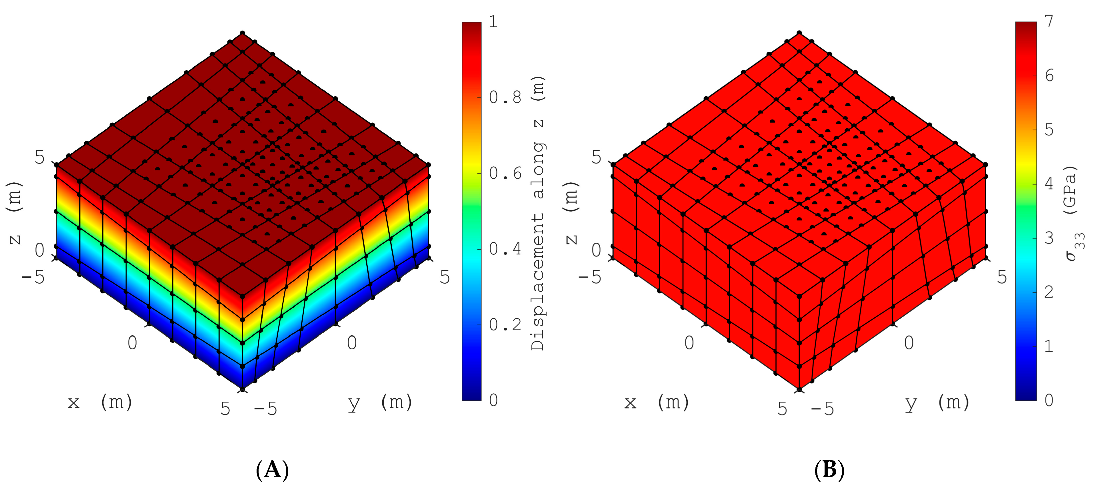
For verification, a specimen of dimension $10 \mathrm{m}\times 10 \mathrm{m}\times 5 \mathrm{m}$ along the $x, y,$ and $z$ axes was modeled and discretized using 256 irregular-shaped linear elements. The element shapes were chosen to be irregular as the patch test would be performed [31]. The material property was chosen as concrete with a modulus of elasticity, density, and Poisson’s ratio of 30 GPa, 3000 $\mathrm{k}\mathrm{g}/{\mathrm{m}}^3$ and 0.3, respectively [32]. One of the elements marked as red in Figure 11A was refined to the fourth order, and the methodology developed in this paper was implemented to transition from the fourth to the first order, as presented in Figure 11B, which produces no hanging nodes. Next, the boundary conditions were applied to restrict the rigid body motions by enforcing displacement $u_x=u_y=u_z=0$ at the $x=0$, $y=0$ and $z=0$ surfaces, respectively, where $u_x$, $u_y$ and $u_z$ show this displacement along the $x, y$ and $z$ axes, respectively. The patch test was performed, wherein a unit displacement $u_z=1$ at all the nodes of the $z=5$ surface was applied, and the static solution was obtained in terms of displacement. The obtained displacement along the $z$ axis is presented in Figure 12A, which shows a linear profile along the $z$ axis throughout the specimen. The displacement $u_z$ was plotted along the $x=y=0$ line, as shown in Figure 13, which shows a linear profile that confirms that the model passed the patch test. The obtained stress profile was also observed as being constant throughout the specimen, as shown in Figure 12B, which provides additional confidence in this method’s capability to produce an accurate solution.

3.3. Implementation of 3D FE Meshes

Two examples are presented in this section. First, the model developed for the verification purpose was subjected to an impact load. Impact load can be replicated through elastic contact modeling [33]. For the sake of simplicity, instead of a contact model, a loading of $F=sin\left(2\pi \mathrm{10,000}t\right)e^{\left(-\mathrm{100,000}t\right)}{10}^{10}$ along the $z$ axis at the central node (T; marked as red in Figure 14) of the refined element was implemented. Such a loading profile can be observed during the cavity expansion at a hypervelocity impact event [34] as presented in Figure 15A. With a timestep [35] of 0.001 mili-s, following the central difference time-stepping algorithm, the displacement profile was obtained. The displacement profiles along z at two nodes (Nodes S and D of Figure 14) are presented in Figure 15B. The distance between nodes T and S is 0.551 m, whereas it is 0.1585 for Node D. It is obvious that, as the distance increases, the wave attenuates. A 3D profile for both displacement and pressure stress profiles is presented in Figure 16, which shows the propagation of the wave in a qualitative manner.

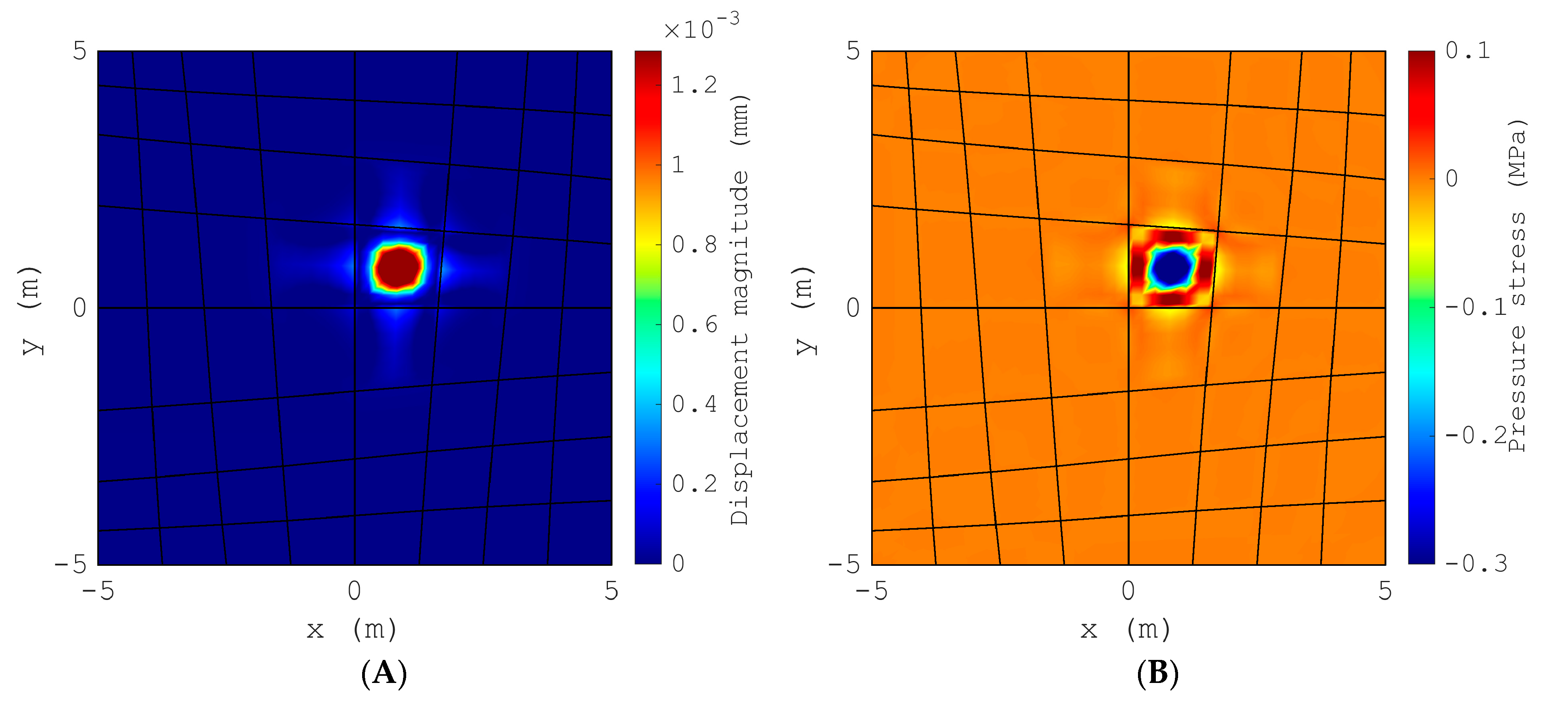
Next, a space habitat model with an outer radius of 2.9 m and an inner radius of 2.5 m is presented. The habitat was discretized into 64 linear elements, as presented in Figure 17A. Scenarios such as meteorite impact cause wave propagation that requires high-density mesh at the impact point. Such action requires re-meshing corresponding to the impact location. Instead of increasing mesh density, higher-order elements offer an excellent solution for simulation wave propagation [8,11,26]. Hence, one of the elements (red in Figure 17B of the model) was enriched to order four, and the procedure developed in this paper was implemented to refine all other elements of the model. The obtained mesh produced no hanging node and a positive definite stiffness matrix. An impact load similar to the previous case perpendicular to the central node of the refined element was implemented. The material property was chosen as aluminum with a modulus of elasticity, density, and Poisson’s ratio of 68 GPa, 2703 $\mathrm{k}\mathrm{g}/{\mathrm{m}}^3$ and 0.3, respectively. The results in terms of radial displacement are presented in Figure 18 for three different distances from the impact node, showing wave decay as distance increases. The nodes T, D, and S follow the same definition as Figure 14, with the distance from T to D and S being 0.0668m and 0.3202, respectively. The 3D profile for displacement norm and pressure stress is also presented in Figure 19A,B, respectively, to provide an overview of the implementation of this method.

4. Conclusions

This paper developed a p-refinement method and a library of six three-dimensional transition elements with the highest order of four, in order to perform p-refinement that gradually decreases polynomial order, element by element, from a refined high-order element. The shape functions and the integration quadratures were computed for each of these elements. The local support and interelement compatibility conditions were checked for each of these elements to verify them. The element properties have been made readily available to FEM users. The p-refinement procedure was tested on irregular mesh, which showed no hanging nodes and passed the patch test. Such refinement is useful in simulating structural vibration due to impact loading, which is presented through two numerical implementations. This development makes local p-refinement possible in 3D finite element applications. The application of these research findings can be extended to the discontinuous Galerkin method applied to wave propagation [6,7], and can help provide competitive results compared to existing methods. Researchers in the field of FEA can benefit by refining only one element to reduce the degrees of freedom. Re-meshing corresponding to the h-refinement can also be avoided, saving computational time and resources.

References

- Zienkiewicz, O.C.; Taylor, R.L.; Zhu, J.Z. The Finite Element Method: Its Basis and Fundamentals; Butterworth Heinemann: Oxford, UK, 2013. [Google Scholar] [CrossRef]
- Bunting, C.F. Introduction to the finite element method. In Proceedings of the 2008 IEEE International Symposium on Electromagnetic Compatibility—EMC 2008, Detroit, MI, USA, 18–22 August 2008; pp. 1–9. [Google Scholar]
- Bathe, K.-J. Discontinuous Finite Element Procedures; Springer: London, UK, 2006; pp. 21–43. [Google Scholar] [CrossRef]
- Ihlenburg, F.; Babuška, I. Finite element solution of the Helmholtz equation with high wave number part I: The h-version of the FEM. Comput. Math. Appl. 1995, 30, 9–37. [Google Scholar] [CrossRef]
- Babuska, I.M.; Sauter, S.A. Is the pollution effect of the FEM avoidable for the Helmholtz equation considering high wave numbers? SIAM J. Numer. Anal. 1997, 34, 2392–2423. [Google Scholar] [CrossRef]
- Baccouch, M.; Temimi, H. A high-order space–time ultra-weak discontinuous Galerkin method for the second-order wave equation in one space dimension. J. Comput. Appl. Math. 2021, 389, 113331. [Google Scholar] [CrossRef]
- Shukla, K.; Chan, J.; de Hoop, M.V.; Jaiswal, P. A weight-adjusted discontinuous Galerkin method for the poroelastic wave equation: Penalty fluxes and micro-heterogeneities. J. Comput. Phys. 2020, 403, 109061. [Google Scholar] [CrossRef]
- Komatitsch, D.; Tromp, J. Spectral-element simulations of global seismic wave propagation-I. Validation. Geophys. J. Int. 2002, 149, 390–412. [Google Scholar] [CrossRef]
- Canuto, C.; Hussaini, M.Y.; Quarteroni, A.; Zang, T.A. Spectral Approximation. In Spectral Methods in Fluid Dynamics; Springer: Berlin/Heidelberg, Germany, 1988; pp. 31–75. [Google Scholar] [CrossRef]
- Palacz, M.; Krawczuk, M.; Żak, A. Spectral Element Methods for Damage Detection and Condition Monitoring. In Advances in Asset Management and Condition Monitoring; Springer: Cham, Switzerland, 2020; pp. 549–558. [Google Scholar]
- Ostachowicz, W.; Kudela, P.; Krawczuk, M.; Zak, A. Guided Waves in Structures for SHM: The Time-Domain Spectral Element Method; John Wiley & Sons, Ltd.: New York, NY, USA, 2012. [Google Scholar] [CrossRef]
- Patera, A.T. A spectral element method for fluid dynamics: Laminar flow in a channel expansion. J. Comput. Phys. 1984, 54, 468–488. [Google Scholar] [CrossRef]
- Ihlenburg, F.; Babuska, I. Finite element solution of the helmholtz equation with high wave number part II: The h-p version of the FEM. SIAM J. Numer. Anal. 1997, 34, 315–358. [Google Scholar] [CrossRef]
- Park, G.-H. P-Refinement Techniques for Vector finite Elements in Electromagnetics. Ph.D. Thesis, Georgia Institute of Technology, Atlanta, GA, USA, 2005. [Google Scholar]
- Salazar-Palma, M. Iterative and Self-Adaptive Finite-Elements in Electromagnetic Modeling; Artech House: Norwood, MA, USA, 1998. [Google Scholar]
- Shahriar, A.; Majlesi, A.; Montoya, A. A General procedure to formulate 3D elements for finite element applications. Computation 2023, 11, 197. [Google Scholar] [CrossRef]
- Staten, M.L.; Jones, N.L. Local refinement of three-dimensional finite element meshes. Eng. Comput. 1997, 13, 165–174. [Google Scholar] [CrossRef]
- Morton, D.J.; Tyler, J.M.; Dorroh, J.R. A new 3D finite element for adaptive h-refinement in 1-irregular meshes. Int. J. Numer. Methods Eng. 1995, 38, 3989–4008. [Google Scholar] [CrossRef]
- Gordon, W.J.; Hall, C.A. Transfinite element methods: Blending-function interpolation over arbitrary curved element domains. Numer. Math. 1973, 21, 109–129. [Google Scholar] [CrossRef]
- Gordon, W.J. Blending-Function Methods of Bivariate and Multivariate Interpolation and Approximation. SIAM J. Numer. Anal. 1971, 8, 158–177. [Google Scholar] [CrossRef]
- Altenbach, J.; Scholz, E. Ableitung von Formfunktionen für finite Standard-und Übergangselemente auf der Grundlage der gemischten Interpolation. Tech. Mech. -Eur. J. Eng. Mech. 1987, 8, 18–30. [Google Scholar]
- Duczek, S.; Saputra, A.; Gravenkamp, H. High order transition elements: The xy-element concept—Part I: Statics. Comput. Methods Appl. Mech. Eng. 2020, 362, 112833. [Google Scholar] [CrossRef]
- Kim, J.H.; Lim, J.H.; Lee, J.H.; Im, S. A new computational approach to contact mechanics using variable-node finite elements. Int. J. Numer. Methods Eng. 2008, 73, 1966–1988. [Google Scholar] [CrossRef]
- Buczkowski, R. 21-node hexahedral isoparametric element for analysis of contact problems. Commun. Numer. Methods Eng. 1998, 14, 681–692. [Google Scholar] [CrossRef]
- Smith, I.M.; Kidger, D.J. Elastoplastic analysis using the 14-node brick element family. Int. J. Numer. Methods Eng. 1992, 35, 1263–1275. [Google Scholar] [CrossRef]
- Soman, R.; Kudela, P.; Balasubramaniam, K.; Singh, S.K.; Malinowski, P. A study of sensor placement optimization problem for guided wave-based damage detection. Sensors 2019, 19, 1856. [Google Scholar] [CrossRef]
- von Winckel, G. Legende-Gauss-Lobatto Nodes and Weights; MathWorks: Natick, MA, USA, 2020; Volume 20. [Google Scholar]
- Arnold, D.N.; Awanou, G. The serendipity family of finite elements. Found. Comput. Math. 2011, 11, 337–344. [Google Scholar] [CrossRef]
- Chari, M.; Salon, S. Numerical Methods in Electromagnetism; Elsevier BV: Amsterdam, The Netherlands, 2000; ISBN 9780126157604. [Google Scholar]
- Taylor, R.L.; Simo, J.C.; Zienkiewicz, O.C.; Chan, A.C.H. The patch test—A condition for assessing FEM convergence. Int. J. Numer. Methods Eng. 1986, 22, 39–62. [Google Scholar] [CrossRef]
- Irons, B.M.; Razzaque, A. Experience with the patch test for convergence of finite elements. In The Mathematical Foundations of the Finite Element Method with Applications to Partial Differential Equations; Elsevier: Amsterdam, The Netherlands, 1972; pp. 557–587. [Google Scholar]
- Rashid, M.A.; Mansur, M.A.; Paramasivam, P. Correlations between mechanical properties of high-strength concrete. J. Mater. Civ. Eng. 2002, 14, 230–238. [Google Scholar] [CrossRef]
- Seok, S.; Shahriar, A.; Montoya, A.; Malla, R.B. A finite element approach for simplified 2D nonlinear dynamic contact/impact analysis. Arch. Appl. Mech. 2023, 93, 3511–3531. [Google Scholar] [CrossRef]
- Sun, Y.; Shi, C.; Liu, Z.; Wen, D. Theoretical research progress in high-velocity/hypervelocity impact on semi-infinite targets. Shock Vib. 2015, 2015, 265321. [Google Scholar] [CrossRef]
- Marfurt, K.J. Accuracy of finite-difference and finite-element modeling of the scalar and elastic wave equations. Geophysics 1984, 49, 533–549. [Google Scholar] [CrossRef]
Figure 1.
Case 1 schematic. Numbers 1–8 indicates the node number for a 8 node brick element.
Figure 2.
Case 2 schematic. Numbers 1–8 indicates the node number for a 8 node brick element.
Figure 3.
Case 3 schematic.
Figure 4.
Renimenet sequence.
Figure 5.
Arbitrary element formulation procedure flowchart.
Figure 6.
Interelement compatibility check between second-order and second-to-first-order transition elements (case 2). (A) Two elements assembled; (B) interelement surface.
Figure 7.
Full-order elements of order (A) 3 and (B) 4.
Figure 8.
Transition elements from order 2 to 1; (A) Case 1; (B) Case 2.
Figure 9.
Transition elements from order 3 to 2; (A) Case 1; (B) Case 2.
Figure 10.
Transition elements from order 4 to 3; (A) Case 1; (B) Case 2.
Figure 11.
Mesh refinement: (A) original mesh; (B) refined mesh following refinement of red marked element to order four (isometric view). Dots represents the nodes.
Figure 12.
(A) Displacement and (B) stress profile for the patch test. Dots represents the nodes.
Figure 13.
Displacement along the axis profile on the line.
Figure 14.
Schematic of impact load and three nodes of interest. Red node T indicates the node to be impacted. Blue and green nodes, D, and T, respectively indicates two neighbouring nodes.
Figure 15.
(A) Force profile and (B) displacement along the z axis at three different nodes.
Figure 16.
Top view of (A) Displacement norm and (B) pressure stress profile at 0.04 mili-sec of the refined mesh.
Figure 17.
(A) Original mesh with 8 node brick element, (B) refined mesh followed by refinement of an element to the fourth order.
Figure 18.
Radial displacement norm at three different nodes.
Figure 19.
Isometric view of (A) Displacement norm and (B) pressure stress profile at 0.35 mili-sec of the refined mesh.