A Novel “Finite Element-Meshfree” Triangular Element Based on Partition of Unity for Acoustic Propagation Problems

Abstract

The accuracy of the conventional finite element (FE) approximation for the analysis of acoustic propagation is always characterized by an intractable numerical dispersion error. With the aim of enhancing the performance of the FE approximation for acoustics, a coupled FE-Meshfree numerical method based on triangular elements is proposed in this work. In the proposed new triangular element, the required local numerical approximation is built using point interpolation mesh-free techniques with polynomial-radial basis functions, and the original linear shape functions from the classical FE approximation are employed to satisfy the condition of partition of unity. Consequently, this coupled FE-Meshfree numerical method possesses simultaneously the strengths of the conventional FE approximation and the meshfree numerical techniques. From a number of representative numerical experiments of acoustic propagation, it is shown that in acoustic analysis, better numerical performance can be achieved by suppressing the numerical dispersion error by the proposed FE-Meshfree approximation in comparison with the FE approximation. More importantly, it also shows better numerical features in terms of convergence rate and computational efficiency than the original FE approach; hence, it is a very good alternative numerical approach to the existing methods in computational acoustics fields.

1. Introduction

Acoustic propagation problems usually play a very important role in many branches of engineering applications. Analytical approaches can only solve relatively simple acoustic problems and usually have obvious limitations in handling relatively complicated acoustic propagations in which very complex geometric shapes are always involved. Therefore, numerical methods are the main approach to tackling complex acoustic propagation problems in practical engineering computations [1,2].

One dominant numerical approach for acoustic propagation analysis is the traditional finite element (FE) approach [3,4]. In comparison with other existing numerical techniques (such as the finite difference method [5,6,7,8], the finite volume method [9], and the mesh-free collocation method [10,11,12,13]), the classical FE approximation in solving acoustic problems, which is usually governed by the Helmholtz equation, has several obvious advantages [14,15]. Firstly, the mathematical background of the FE approximation is quite firm in handling various partial differential equations, and various boundary conditions (BCs) (including the Dirichlet BCs and Neumann BCs) can be properly imposed. Secondly, owing to the local feature of the FE approximation, the constructed system matrices for the governing equation are always sparse and banded; hence, the practical computation process can be significantly speeded up, and the required memory space can also be markedly reduced. Additionally, the acoustic propagation in nonhomogeneous media can be directly handled by the FE approximation, and the coupling of the acoustic propagation with other complex structures can be realized naturally. Nevertheless, the FE approach still possesses several inherent drawbacks in acoustic analysis. One important issue is the numerical dispersion error, which is essentially a particularity of the Helmholtz equation and generally cannot be totally removed [15]. Due to this issue, the conventional FE approach is usually limited to solving acoustic problems in a relatively low frequency range. For the purpose of controlling the numerical dispersion error, in the computation process we have to adopt the mesh size according to the computed frequency values, such that sufficient elements are employed to discretize one wavelength. With this approach, the required computation expenses will increase dramatically when the computed frequency gets higher.

Actually, the numerical error of the FE solutions for acoustics is mainly made up of two different components, namely the error component from the pollution effects (or dispersion effects in several literatures) and the numerical interpolation error component [16,17]. The concept of interpolation error in acoustic problems is similar to that in standard elasticity and thermal problems [18,19]. This error component will converge at the same rate as the decrease in the average mesh size or nodal space in the local region. The FEM researchers usually believe that this error can be suppressed if the used acoustic wave resolution n ($n=\lambda /h$, in which $\lambda$ is the wavelength and $h$ is the average nodal space) is sufficiently large to approximate the solution. However, the behavior of the error component from the dispersion effects is identified to be much more complex; it is actually global in nature, and it could degrade the quality of the numerical solutions everywhere in the considered problem domain [19]. Although the acoustic wave resolution n is large enough, the dispersion error will never vanish. In order to effectively address the numerical error issue, many improved and modified FE approximations (such as the smoothed FEM [20,21,22,23,24,25], generalized FEM [26,27] and enriched FEM [28,29,30]) have been developed, and quite tremendous progress has been achieved. However, the numerical dispersion error can still not be totally removed [31,32,33,34,35].

In addition to the classical FE approximation approach, boundary element and boundary-based techniques are also effective numerical approaches for acoustic propagation analysis [36,37,38,39,40]. Compared to the FE approach, only the boundary discretization is needed in these boundary-based methods, and the considered problem in d–dimensions can be reduced to a d − 1 dimensional problem [41,42,43,44,45,46,47,48,49], hence the scale of the constructed system matrix equation is clearly smaller than that in the FE approach. However, these obtained system matrices are always dense and non-sparse; hence, the storage and treatment of these system matrices are not as easy as in the FE approach.

Compared to classical FEM, mesh-free approaches are relatively new numerical techniques for solving acoustic problems [50,51,52]. The earliest concept of mesh-free technique is the well-known smooth particle hydrodynamics (SPH), which was first proposed by Lucy et al. [53] to handle astrophysics and fluid dynamics. In the subsequent few decades, several famous mesh-free methods have emerged in modern computational mechanics with considerable success [54,55]. Due to the relatively high degree of accuracy property and independence of the mesh grid, mesh-free numerical techniques have been extensively used for practical engineering computation [54,56,57].

In recent years, mesh-free methods have also been exploited to tackle acoustic problems. Suleau and Bouillard used the element-free Galerkin (EFG) method to solve acoustic wave propagation problems [58]. The numerical results show that the behaviors of the EFG in handling acoustics are quite similar to those of the standard FEM, while the EFG results are much better. Later, Sulear et al. performed the dispersion analysis of the EFG method for acoustics in two dimensions [59]. It is found that it is possible to immensely reduce the pollution error and to obtain fairly good solutions compared to the solutions from FEM as long as the related parameters are carefully chosen. Wenterodt and Estorff focused on using the radial point interpolation technique to study the pollution error issue in acoustic computation [60]. Likewise, a significant reduction of the pollution effects could be achieved, and extremely good numerical solutions could be obtained. In summary, though the mesh-free method is indeed effective in controlling the pollution error, it also has its own disadvantages [61,62,63]. To effectively control the pollution error, too many extra parameters are usually required to be carefully determined; it might be a little difficult for the inexperienced researcher. In addition, several mesh-free techniques usually have difficulties imposing the essential boundary condition [54,64].

The main objective of this work is to introduce a coupled “FE-Meshfree” numerical technique based on ordinary triangular meshes for the analysis of acoustic wave propagation problems. In the proposed new triangular element, the required local numerical approximation is built using point interpolation mesh-free techniques with polynomial-radial basis functions, and the original linear shape functions from the classical FE approximation are employed to satisfy the condition of partition of unity. Owing to the fact that the meshfree techniques usually have relatively high computation precision and the FE approach is easy to carry out, this coupled FE-Meshfree numerical method possesses simultaneously the strengths of the conventional FE approximation and the meshfree numerical techniques. From a number of representative numerical experiments of acoustic propagation, it is shown that in acoustic analysis, better numerical performance can be achieved by suppressing the numerical dispersion error by the proposed FE-Meshfree approximation in comparison with the FE approximation.

2. Weak Form Formulation for Time-Harmonic Acoustics

Assuming that the problem domain $\Omega$ is filled with a homogeneous acoustic medium. $\Gamma$ is the problem domain boundary, and c is the acoustic speed in the medium. With the assumption of small perturbations, the governing equation for acoustic propagation can be obtained as [3,65,66]

$${\nabla }^{2}P-\frac{1}{c^2}\frac{{\partial }^{2}P}{\partial t^2}=0,$$

(1)

in which $P$ and $t$ respectively denote the unknown acoustic pressure field and time.

If the considered acoustic propagation is time-harmonic, we have

$$P=p\exp \left(j\omega t\right),$$

(2)

in which $p$ is amplitude of the acoustic pressure distribution, $\omega$ denotes the angular frequency.

The time variable t in Equation (1) can be eliminated by using Equation (2), and then the governing differential equation becomes

$${\nabla }^{2}p+k^{2}p=0,$$

(3)

where $k=\omega /c$ is the wave number.

In addition, the following equation should also be satisfied for acoustic propagation:

$$\nabla p+j\rho \omega v=0,$$

(4)

in which $\nabla p$ is the acoustic pressure gradient, $v$ is acoustic particle velocity, $\rho$ denotes the acoustic medium density.

When the appropriate boundary conditions (BCs) are applied, the above-described acoustic problem can be completely defined. For acoustic analysis, the boundary $\Gamma$ usually consists of three different types, namely

$${\Gamma =\Gamma }_{\mathrm{D}}\cup {\Gamma }_{\mathrm{N}}\cup {\Gamma }_{\mathrm{R}},$$

(5)

in which ${\Gamma }_{\mathrm{D}}$, ${\Gamma }_{\mathrm{N}}$ and ${\Gamma }_{\mathrm{R}}$ are respectively the Dirichlet, Neumann, and Robin BCs.

The three types of BC are described by the following equations:

$$\left\{\begin{array}{ll}p=\overline{p}& \mathrm{on}{\Gamma }_{\mathrm{D}}\\ v_n=\overline{v}& \mathrm{on}{\Gamma }_{\mathrm{N}}\\ \nabla p=-j\rho \omega A_{n}p& \mathrm{on}{\Gamma }_{\mathrm{R}}\end{array}\right.,$$

(6)

In which $\overline{p}$ and $\overline{v}$ denote the prescribed pressure and velocity on the corresponding boundaries, $v_n$ is the normal particle velocity, and $A_n$ is the admittance coefficient.

With the conventional Galerkin method and applying the above-mentioned three BCs, the standard weak form for acoustic problems can be written as [65,66]

$$-{\displaystyle {\int }_{\Omega }\nabla N·}\nabla Np\mathrm{d}\Omega +k^2{\displaystyle {\int }_{\Omega }N}·Np\mathrm{d}\Omega -i\rho \omega {\displaystyle {\int }_{{\Gamma }_N}N·v_n\mathrm{d}\Gamma }-j\rho \omega A_n{\displaystyle {\int }_{{\Gamma }_R}N·Np\mathrm{d}\Gamma }=0,$$

(7)

where $N$ is the defined nodal interpolation functions.

The considered field variable could be approximated in terms of the corresponding nodal values and interpolation functions in the standard FE analysis.

$$p={\displaystyle \sum N_i{p}_i}=Np,$$

(8)

Using Equation (8), we can arrive at the matrix equation,

$$\left[K-k^{2}M+j\rho \omega C\right]\left[p\right]=-j\rho \omega \left[F\right],$$

(9)

where $K$, $M$ and $C$ represent the system stiffness, mass, and damping matrices.

$$\left\{\begin{array}{l}K={\displaystyle {\int }_{\Omega }{\left(\nabla N\right)}^T}\left(\nabla N\right)\mathrm{d}\Omega \\ M={\displaystyle {\int }_{\Omega }{N}^T}N\mathrm{d}\Omega \\ C={\displaystyle {\int }_{{\Gamma }_{\mathrm{R}}}{A}_n{N}^T}N\mathrm{d}\Gamma \\ F={\displaystyle {\int }_{{\Gamma }_{\mathrm{N}}}{N}^T}{v}_n\mathrm{d}\Gamma \end{array}\right.,$$

(10)

3. Construction of the Coupled “FE-Meshfree” Numerical Approximation

In constructing the present “FE-Meshfree” numerical approximation, the partition of unity (PU) condition is used, and the conventional FE interpolation functions are directly used as the required non-negative weight functions. Based on the PU condition, we have

$${\displaystyle \sum w_i\left(x\right)=1},$$

(11)

in which $w_i\left(x\right)$ stands for the weight function for node i.

Then the global numerical approximation $u_h\left(x\right)$ in the proposed “FE-Meshfree” framework can be constructed as

$$u_h\left(x\right)={\displaystyle \sum _{i=1}^n{w}_i\left(x\right)u_i\left(x\right)},$$

(12)

in which n is the number of involved nodes and $u_i\left(x\right)$ denotes the constructed local numerical approximation for node i.

From Equation (12), it is seen that the main difference between the present numerical approximation and the FE approximation is the local numerical approximation for each node. In the FE approach, the nodal unknowns are directly used as the local approximation, while in the proposed method, the newly constructed local numerical approximation is used. In this work, the required local numerical approximation is built using mesh-free techniques.

Actually, various numerical techniques can be utilized to build the required local numerical approximation. Due to the Kronecker-delta function property and relatively high computation precision, the polynomial-radial base functions in the mesh-free point interpolation method with radial base functions (RPIM) are employed to form the local nodal numerical approximation. Here the nodal interpolation function in the RPIM is first introduced briefly.

If there are m field nodes in the defined support domain for node i, the required local nodal numerical approximation is constructed by [54]

$$u\left(x\right)={\displaystyle \sum _{i=1}^m{R}_i\left(x\right)a_i+{\displaystyle \sum _{j=1}^3{q}_j\left(x\right)b_j}}=R^T\left(x\right)a+q^T\left(x\right)b,$$

(13)

in which $a_i$ and $b_j$ are the associated unknown interpolation coefficients, $R_i\left(x\right)$ and $q_j\left(x\right)$ are respectively the radial and polynomial base functions.

In this work, we only use the linear polynomial base functions in two-dimensional space, namely

$$q=\left[\begin{array}{ccc}1& x& y\end{array}\right],$$

(14)

The employed multi-quadric radial base functions have the following form:

$$\left\{\begin{array}{l}{R}^T\left(x\right)=\left[\begin{array}{ccccc}{R}_1\left(x\right)& R_2\left(x\right)& R_3\left(x\right)& \dots & R_n\left(x\right)\end{array}\right]\\ R_i\left(x\right)={\left[r_i^2+{\left({\alpha }_c{d}_c\right)}^2\right]}^q\\ r_i=\sqrt{{\left(x-x_i\right)}^2+{\left(y-y_i\right)}^2}\end{array}\right.,$$

(15)

in which $d_c$ is the node space of the used node distribution, ${\alpha }_c$ and $q$ are two important parameters that can be determined from Ref. [51].

If the numerical approximation in Equation (13) is satisfied for all m field nodes in the support domain, we have

$$u\left(x\right)={\displaystyle \sum _{i=1}^m{R}_i}\left(x\right)a_i+{\displaystyle \sum _{j=1}^3{p}_j}\left(x\right)b_j=Ra+Qb,$$

(16)

$$R={\left[\begin{array}{cccc}{R}_1\left(r_1\right)& R_2\left(r_1\right)& \cdots & R_n\left(r_1\right)\\ R_1\left(r_2\right)& R_2\left(r_2\right)& \cdots & R_n\left(r_2\right)\\ ⋮& ⋮& \ddots & ⋮\\ R_1\left(r_m\right)& R_2\left(r_m\right)& \cdots & R_m\left(r_m\right)\end{array}\right]}_{m\times m},$$

(17)

$$Q=\left[\begin{array}{cccc}{P}_1\left(x_1\right)& P_2\left(x_1\right)& \cdots & P_m\left(x_1\right)\\ P_1\left(x_2\right)& P_2\left(x_2\right)& \cdots & P_m\left(x_2\right)\\ P_1\left(x_3\right)& P_2\left(x_3\right)& \cdots & P_m\left(x_3\right)\end{array}\right],$$

(18)

From Ref. [54], it is known that the determination of the unknown interpolation coefficients $a$ and $b$ also requires the following restrictions:

$${\displaystyle \sum _{i=1}^m{q}_j}\left(x_i\right)a_i=0, j=1,2,3,$$

(19)

Then the numerical approximation in Equation (16) can finally be written by

$$\left\{\begin{array}{l}{u}_h\left(x\right)=R^T\left(x\right)a+q^T\left(x\right)b=\left[R^T\left(x\right)S_a+Q^T\left(x\right)S_b\right]u_s=\Phi \left(x\right)u\\ S_a=\left(R^{-1}-R^{-1}Q{S}_b\right)\\ S_b=\left[Q^T{R}^{-1}Q\right]Q^T{R}^{-1}\end{array}\right.,$$

(20)

in which $\Phi \left(x\right)$ is the constructed polynomial-radial node shape function in the RPIM.

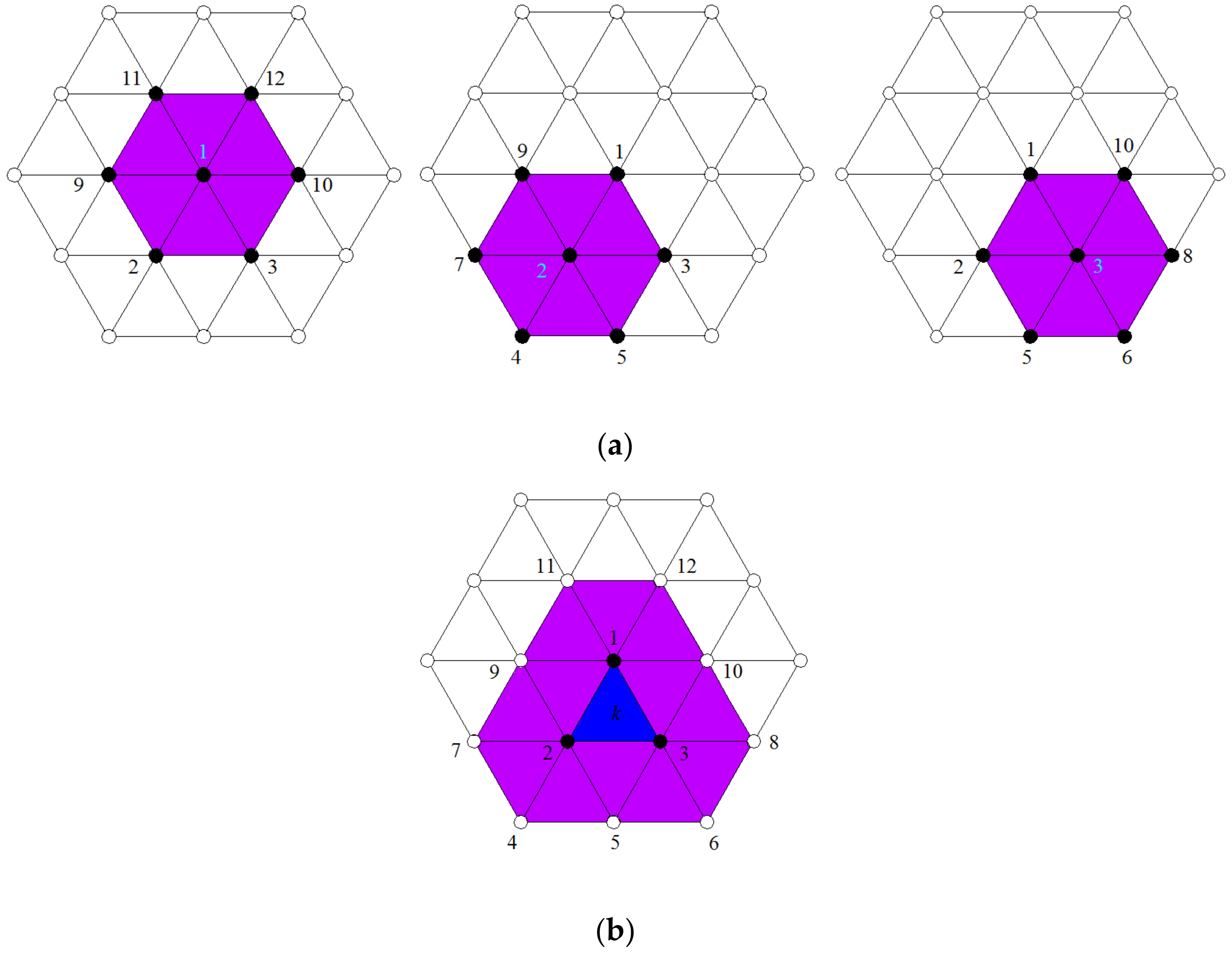
In the present coupled “FE-Meshfree” triangular element, the required numerical approximation is constructed by using composite nodal interpolation functions, which are formed by combining the conventional FE and RPIM interpolation functions [67,68,69,70]. The former is designed to fulfill the PU condition, and the latter is employed to build the required local nodal approximation; hence, the abbreviation Trig3-RPIM is used to denote this coupled “FE-Meshfree” triangular element. To clearly show the formulation of the present Trig3-RPIM element, the support domains for each node and element are defined here (see Figure 1). The node support contains all elements sharing the mutual node, and the element support denotes the domains containing all the associated node supports.

By combining Equations (12) and (13), for the element containing M field nodes, the constructed numerical approximation for this Trig3-RPIM is expressed as

$$\left\{\begin{array}{l}p\left(x\right)=N\left(\Phi p\right)=\left(N\Phi \right)p=\Psi p\\ \Psi =[{\psi }_1, {\psi }_2 ,\dots , {\psi }_M]=\underset{1\times 3}{\underbrace{N}}\underset{3\times M}{\underbrace{\Phi }}\\ p=[p_1, p_2 ,\dots , p_M]\end{array}\right.,$$

(21)

where $\Psi$ represents the constructed composite interpolation functions for this Trig3-RPIM element.

For the node arrangement in Figure 1, the purple region represents the local node support ${\Omega }_1$ = {1, 2, 3, 10, 12, 11, 9} for node 1. Similarly, the node supports for node 2 and node 3 are ${\Omega }_2$ = {2, 4, 5, 3, 1, 9, 7} and ${\Omega }_3$ = {3, 5, 6, 8, 10, 1, 2}, respectively. In Equation (21), the global numerical approximation is given by

$$p\left(x\right)=N_1{p}_1\left(x\right)+N_2{p}_2\left(x\right)+N_3{p}_3\left(x\right),$$

(22)

Following the formulation of the original RPIM approximation [54,71], the local numerical approximation is expressed by

$$\left\{\begin{array}{l}{p}_1\left(x\right)={\Phi }_1^1{p}_1+{\Phi }_2^1{p}_2+{\Phi }_3^1{p}_3+{\Phi }_{10}^1{p}_{10}+{\Phi }_{12}^1{p}_{12}+{\Phi }_{11}^1{p}_{11}+{\Phi }_9^1{p}_9\\ p_2\left(x\right)={\Phi }_2^2{p}_2+{\Phi }_4^2{p}_4+{\Phi }_5^2{p}_5+{\Phi }_3^2{p}_3+{\Phi }_1^2{p}_1+{\Phi }_9^2{p}_9+{\Phi }_7^2{p}_7\\ p_3\left(x\right)={\Phi }_3^3{p}_3+{\Phi }_5^3{p}_5+{\Phi }_6^3{p}_6+{\Phi }_8^3{p}_8+{\Phi }_{10}^3{p}_{10}+{\Phi }_1^3{p}_1+{\Phi }_2^3{p}_2\end{array}\right.,$$

(23)

in which $p_i$ denotes nodal acoustic pressure and ${\Phi }_i^j$ stands for the corresponding nodal shape function based on the RPIM formulation.

Then the interpolation function matrix $\Phi$ in Equation (21) can be expressed by

$$\Phi =\left[\begin{array}{cccccccccccc}{\Phi }_1^1& {\Phi }_2^1& {\Phi }_3^1& 0& 0& 0& 0& 0& {\Phi }_9^1& {\Phi }_{10}^1& {\Phi }_{11}^1& {\Phi }_{12}^1\\ {\Phi }_1^2& {\Phi }_2^2& {\Phi }_3^2& {\Phi }_4^2& {\Phi }_5^2& 0& {\Phi }_7^2& 0& {\Phi }_9^2& 0& 0& 0\\ {\Phi }_1^3& {\Phi }_2^3& {\Phi }_3^3& 0& {\Phi }_5^3& {\Phi }_6^3& 0& {\Phi }_8^3& 0& {\Phi }_{10}^3& 0& 0\end{array}\right],$$

(24)

Finally, the composite interpolation matrix $\Psi$ can be expressed by

$$\Psi =N\Phi ={\left[\begin{array}{c}{N}_1\\ N_2\\ N_3\end{array}\right]}^T\left[\begin{array}{cccccccccccc}{\Phi }_1^1& {\Phi }_2^1& {\Phi }_3^1& 0& 0& 0& 0& 0& {\Phi }_9^1& {\Phi }_{10}^1& {\Phi }_{11}^1& {\Phi }_{12}^1\\ {\Phi }_1^2& {\Phi }_2^2& {\Phi }_3^2& {\Phi }_4^2& {\Phi }_5^2& 0& {\Phi }_7^2& 0& {\Phi }_9^2& 0& 0& 0\\ {\Phi }_1^3& {\Phi }_2^3& {\Phi }_3^3& 0& {\Phi }_5^3& {\Phi }_6^3& 0& {\Phi }_8^3& 0& {\Phi }_{10}^3& 0& 0\end{array}\right],$$

(25)

From the above formulation, the complete numerical approximation of the present Finite element-Meshfree can be written by

$$\begin{array}{ll}p\left(x\right)& =\Psi p=N\Phi p\\ & ={\left[\begin{array}{c}{N}_1\\ N_2\\ N_3\end{array}\right]}^T\left[\begin{array}{cccccccccccc}{\Phi }_1^1& {\Phi }_2^1& {\Phi }_3^1& 0& 0& 0& 0& 0& {\Phi }_9^1& {\Phi }_{10}^1& {\Phi }_{11}^1& {\Phi }_{12}^1\\ {\Phi }_1^2& {\Phi }_2^2& {\Phi }_3^2& {\Phi }_4^2& {\Phi }_5^2& 0& {\Phi }_7^2& 0& {\Phi }_9^2& 0& 0& 0\\ {\Phi }_1^3& {\Phi }_2^3& {\Phi }_3^3& 0& {\Phi }_5^3& {\Phi }_6^3& 0& {\Phi }_8^3& 0& {\Phi }_{10}^3& 0& 0\end{array}\right]\left[\begin{array}{l}{p}_1\\ p_2\\ ⋮\\ p_{12}\end{array}\right]\end{array}$$

(26)

In the Cartesian coordinate system, the derivatives of $\Psi$ for triangular element can be directly obtained by

$$\left\{\begin{array}{l}{\Psi }_{,x}=N_{,x}\Phi +N{\Phi }_{,x}\\ {\Psi }_{,y}=N_{,y}\Phi +N{\Phi }_{,y}\end{array}\right.,$$

(27)

The size of the derivatives ${\Psi }_{,x}$ and ${\Psi }_{,y}$ is $3\times M$. After obtaining the related derivatives of the interpolation functions, the related system matrices can be calculated directly. It should be noted that the Gauss integration rule is still used for numerical integration in the present method, which is very similar to the traditional FE scheme.

With the above formulations, the discrete governing equations for acoustic propagation problems using the present Finite element-meshfree approximation can be expressed by

$$\left[\overline{K}-k^2\overline{M}+j\rho \omega \overline{C}\right]\left[p\right]=-j\rho \omega \left[\overline{F}\right],$$

(28)

in which $\overline{K}$, $\overline{M}$, $\overline{C}$, and $\overline{F}$ denote the corresponding system matrices and nodal vectors obtained by the present Finite element-Meshfree method.

$$\left\{\begin{array}{l}K={\displaystyle {\int }_{\Omega }{\left(\nabla \Psi \right)}^T}\left(\nabla \Psi \right)\mathrm{d}\Omega ={\displaystyle {\int }_{\Omega }{\left[\nabla \left(N\Phi \right)\right]}^T}\left[\nabla \left(N\Phi \right)\right]\mathrm{d}\Omega \\ M={\displaystyle {\int }_{\Omega }{\Psi }^T}\Psi \mathrm{d}\Omega ={\displaystyle {\int }_{\Omega }{\left(N\Phi \right)}^T}\left(N\Phi \right)\mathrm{d}\Omega \\ C={\displaystyle {\int }_{{\Gamma }_{\mathrm{R}}}{A}_n{\Psi }^T}\Psi \mathrm{d}\Gamma ={\displaystyle {\int }_{{\Gamma }_{\mathrm{R}}}{A}_n{\left(N\Phi \right)}^T}\left(N\Phi \right)\mathrm{d}\Gamma \\ F={\displaystyle {\int }_{{\Gamma }_{\mathrm{N}}}{\Psi }^T}{v}_n\mathrm{d}\Gamma ={\displaystyle {\int }_{{\Gamma }_{\mathrm{N}}}{\left(N\Phi \right)}^T}{v}_n\mathrm{d}\Gamma \end{array}\right.,$$

(29)

From Equations (10) and (29), it is seen that in the present method, the standard finite element nodal shape function $N$ is replaced by the composite nodal shape function $\Psi$, which is actually a combination of the standard finite element nodal shape function $N$ and the RPIM mesh-free nodal shape function $\Phi$.

The comparisons of the influencing domain and interpolation functions for one node in the traditional FEM-T3 and the proposed Trig3-RPIM are given in Figure 2. We can observe that if a larger influencing domain is used in the Trig3-RPIM compared to the FEM-T3, then more field nodes will be involved in constructing the numerical approximation. We can also see that the present Trig3-RPIM has smoother nodal interpolation functions than the FEM-T3 due to the fact that a higher-order numerical approximation can be achieved in this Trig3-RPIM. Therefore, it is quite reasonable to expect that the coupled numerical approximation in this Trig3-RPIM element is more suitable to approximate the acoustic wave propagation problems and that less numerical error can be obtained compared to the traditional FE approach.

It is important to note that the composite nodal interpolations employed here also have the Kronecker-delta function property. This good numerical feature is acquired by the fact that the RPIM has this important numerical feature. A brief proof of this is given as follows:

Based on Equation (21), for a conventional triangular element, the constructed composite nodal interpolations are written by

$$\Psi =\left[\begin{array}{ccc}{N}_1& N_2& N_3\end{array}\right]\left[\begin{array}{ccccc}{\varphi }_1^1& {\varphi }_2^1& {\varphi }_3^1& \cdots & {\varphi }_M^1\\ {\varphi }_1^2& {\varphi }_2^2& {\varphi }_3^2& \cdots & {\varphi }_M^2\\ {\varphi }_1^3& {\varphi }_2^3& {\varphi }_3^3& \cdots & {\varphi }_M^3\end{array}\right],$$

(30)

If node 1 has the coordinate values $\left(x,y\right)=\left(x_1,y_1\right)$, the values of the interpolation function at node 1 can be calculated as follows:

$$\Psi =\left[\begin{array}{ccc}1& 0& 0\end{array}\right]\left[\begin{array}{ccccc}1& 0& 0& \cdots & 0\end{array}\right]\hspace{1em}\hspace{1em} \mathrm{at} \mathrm{node} 1,$$

(31)

Equation (28) means that

$$\underset{1\times M}{\underbrace{\Psi }}=\left[\begin{array}{ccccc}1& 0& 0& \cdots & 0\end{array}\right]\hspace{1em}\hspace{1em} \mathrm{at} \mathrm{node} 1,$$

(32)

Using the similar way, for nodes 2 and 3, we have

$$\left\{\begin{array}{ll}\underset{1\times M}{\underbrace{\Psi }}=\left[\begin{array}{ccccc}1& 0& 0& \cdots & 0\end{array}\right]& \hspace{1em}\hspace{1em}\mathrm{at} \mathrm{node} 2\\ \underset{1\times M}{\underbrace{\Psi }}=\left[\begin{array}{ccccc}0& 1& 0& \cdots & 0\end{array}\right]& \hspace{1em}\hspace{1em}\mathrm{at} \mathrm{node} 3\end{array}\right.,$$

(33)

From the above formulation, it is seen that the Kronecker-delta function property is indeed maintained by the present composite nodal interpolation functions, which make it quite easy to apply the essential boundary conditions.

4. Numerical Examples

Several typical acoustic wave propagation problems are solved with various numerical techniques in this section to test the behaviors of the present Trig3-RPIM element. In addition to the traditional FEM-T3, edge-based smoothed FEM (ES-FEM) [65] and RPIM (ES-RPIM) [72] have also been used here for a clear comparison and discussion. We can observe that the proposed Trig3-RPIM element works well for the acoustic propagation problem; meanwhile, it also has stronger abilities than other mentioned methods in terms of computation efficiency and convergence rate. To effectively evaluate the obtained numerical solutions, the following error estimator is defined:

$$e_n=\sqrt{{\displaystyle {\int }_{\Omega }{\left({\overline{v}}_e-{\overline{v}}_h\right)}^T\left(v_e-v_h\right)\mathrm{d}\Omega }},$$

(34)

where $v_e$ and $v_h$ are the exact and numerical acoustic particle velocities, and the overbar means the complex conjugate values.

The global relative error indicator is defined by

$$\eta =\sqrt{\frac{{\displaystyle {\int }_{\Omega }{\left({\overline{v}}_e-{\overline{v}}_h\right)}^T\left(v_e-v_h\right)\mathrm{d}\Omega }}{{\displaystyle {\int }_{\Omega }{\overline{v}}^T{v}_e\mathrm{d}\Omega }}},$$

(35)

4.1. Acoustic Propagation in a 2D Tube

As shown in Figure 3, the acoustic wave propagation in a 2D tube is solved here. The tube is filled with water (acoustic wave speed c = 1500 m/s and fluid density $\rho$ = 1000 kg/m³). The geometry configuration of this 2D tube is width b = 0.1 m and length l = 1 m. The Neumann BC with $v_n$ = 1 m/s is applied to the left side, and the other sides are assumed to be completely rigid. The employed mesh pattern for this considered problem is shown in Figure 4. The exact acoustic particle velocity and pressure are given by

$$\left\{\begin{array}{l}p=-j\rho c{v}_n\frac{\cos \left[k\left(1-x\right)\right]}{\sin \left(k\right)}\\ v=v_n\frac{v_n\sin \left[k\left(1-x\right)\right]}{\sin \left(k\right)}\end{array}\right.,$$

(36)

In addition, the eigenfrequencies of this problem are given by

$$f=\frac{c}{2}\sqrt{{\left(\frac{m}{l}\right)}^2+{\left(\frac{n}{b}\right)}^2} m,n=0, 1, 2, 3 \cdots ,$$

(37)

4.1.1. Computation Accuracy Study

We first showed the pressure distributions at disparate frequency values along the x-axis using various methods (see Figure 5). We note that all the methods used can basically produce fairly good results when the frequency value f = 2000 Hz. If the frequency value becomes higher (f = 4000 Hz and f = 7000 Hz), all the numerical solutions will gradually depart from the analytical solutions. However, it clearly appears that the present Trig3-RPIM can provide the most accurate solutions. This is because the high-order numerical approximation can be constructed by the Trig3-RPIM, hence the potential numerical errors can be largely suppressed.

Furthermore, the acoustic eigenfrequency analysis of this 2D tube is also carried out here.

Table 1. The first fifteen eigenfrequency values of the 2D tube.

Mode	Exact (Hz)	Trig3-RPIM (Hz)	Trig3-RPIM Error(%)	FEM-T3 (Hz)	FEM-T3 Error(%)	ES-FEM (Hz)	ES-FEM Error(%)
1	750.00	749.99	0.00	750.12	0.02	750.06	0.01
2	1500.00	1499.77	0.02	1500.99	0.07	1500.74	0.05
3	2250.00	2249.23	0.03	2253.33	0.15	2252.69	0.12
4	3000.00	2998.18	0.06	3007.90	0.26	3006.53	0.22
5	3750.00	3746.49	0.09	3765.44	0.41	3762.87	0.34
6	4500.00	4494.02	0.13	4526.69	0.59	4522.28	0.50
7	5250.00	5240.67	0.18	5292.41	0.81	5285.36	0.67
8	6000.00	5986.34	0.23	6063.35	1.06	6052.65	0.88
9	6750.00	6730.99	0.28	6840.26	1.34	6824.65	1.11
10	7500.00	7474.57	0.34	7623.90	1.65	7601.81	1.36
11	7500.00	7547.38	0.63	7623.90	1.65	7622.74	1.64
12	7537.40	7584.21	0.62	7670.71	1.77	7663.63	1.67
13	7648.50	7693.12	0.58	7798.25	1.96	7786.83	1.81
14	7830.20	7871.27	0.52	7999.93	2.17	7988.40	2.02
15	8077.70	8113.91	0.45	8295.81	2.70	8263.10	2.30

lists the first fifteen eigenfrequency values obtained from disparate methods. From the results in the table, it is found that all the employed methods can provide relatively accurate eigenfrequency values for the low-mode orders. Due to the numerical error issue, the computation accuracy for the eigenfrequency value will degenerate quickly when the mode order becomes higher. Nevertheless, the Trig3-RPIM can stand out clearly among all the numerical methods, and the most accurate eigenfrequency values can be predicted, particularly when the mode order is relatively high. The above observations mean that the Trig3-RPIM clearly surpasses the other methods in dealing with the acoustic propagation problems.

4.1.2. Convergence Rate Study

This sub-section aims at testing the convergence rate of the Trig3-RPIM in acoustic analysis. When the frequency value f = 2000 Hz, the obtained global numerical error results from disparate methods using varying mesh patterns are plotted in Figure 6. We can see that the Trig3-RPIM can not only converge faster than the FEM-T3, but also behave better than the ES-FEM and ES-RPIM. These findings indicate that the proposed Trig3-RPIM also has better numerical performance than the other employed methods in terms of convergence properties.

4.1.3. Computational Efficiency Study

The computation accuracy and convergence rate studies have been carried out in previous sections, and it is seen that the Trig3-RPIM indeed has excellent performance compared to other methods. However, whether it still behaves better in terms of computational efficiency is still not very clear. This sub-section aims at examining the computational efficiency of the Trig3-RPIM in acoustic analysis. Here the varying mesh pattern with disparate element sizes is again employed, and the frequency value f = 4400 Hz.

Figure 7 shows the CPU time, which is employed to denote the computational efforts, against the global error indicator from disparate methods. We can see that the required CPU time will increase if the refined meshes are employed. Meanwhile, the present Trig3-RPIM seems to be significantly more expensive than the other methods employed with a totally identical mesh pattern. These findings reveal that the relatively high computation accuracy and fast convergence rate of the Trig3-RPIM are not free of any expenses. It is not difficult to understand this because there are mainly two factors contributing to the expensiveness of the Trig3-RPIM. One reason is that more expensive numerical integration should be carried out because higher-order numerical approximation is always involved in this Trig3-RPIM element. Another reason is that in this Trig3-RPIM, the half-bandwidth of the system matrices is always much larger than that in other methods because more field nodes will be involved in constructing the system matrices. Therefore, more memory space is needed to store the system matrices, and more computational efforts will be required to implement the related matrix inversion process. However, it is quite interesting to note that the Trig3-RPIM is actually a winner compared to other methods when we take computation accuracy into consideration because less CPU time is required when the Trig3-RPIM is used for acoustic computation for the identical computation accuracy. This indicates that the Trig3-RPIM also has higher computational efficiency than the other methods used in acoustic analysis. This attractive numerical feature will further strengthen the application prospects of the proposed Trig3-RPIM for solving acoustic wave propagation problems.

4.2. Acoustic Propagation in a Square Domain

Here we consider a 2D square domain (length L = 1 m, acoustic medium density =1.25 kg/m³, and acoustic wave speed c = 340 m/s) with Robin BC (see Figure 8). The Dirichlet BC with pressure p = 1 Pa is applied at the bottom left corner. Figure 9 gives the employed mesh pattern with regular (structured mesh) and irregular (unstructured mesh) node distributions for this problem. Likewise, it is not difficult to obtain the corresponding exact solution, which is given by

$$p=\cos \left[k\left(x\cos \beta +y\sin \beta \right)\right]+j\sin \left[k\left(x\cos \beta +y\sin \beta \right)\right],$$

(38)

in which $\beta$ represents the angle of acoustic wave propagation.

Firstly, we examine the performance of different methods by investigating their sensitivity to the geometry distortion of the used mesh. To achieve this objective, both structured and unstructured meshes with a completely identical total node number, as shown in Figure 9, are used for numerical computation. For the frequency value f = 380 Hz and acoustic wave propagation angle $\beta =45°$, Figure 10 shows the calculated acoustic pressure distribution along the diagonal line of the problem domain. It is observed that the linear FEM-T3 solutions are notably affected by the unstructured mesh; both ES-FEM and ES-RPIM have considerable abilities in tackling the mesh distortion, and the corresponding numerical solutions are clearly more accurate than the FEM-T3. Nevertheless, it is very interesting to see that the Trig3-RPIM solutions are closest to the exact ones, and almost identical solutions are produced when the structured and unstructured meshes are utilized. These findings indicate that the Trig3-RPIM is basically immune from mesh distortion, which is a distinct advantage over the other methods in acoustic computation. This is probably because the local numerical approximation in the Trig3-RPIM is constructed using mesh-free techniques.

Furthermore, the numerical errors of different methods in tackling this 2D acoustic problem are studied by using regular meshes with different element sizes. The numerical error results are plotted in Figure 11. For the convenience of discussion, $k^3{h}^2=1$ and $kh=1$ are also shown in Figure 11. It is quite easy to find that the numerical errors are quite small when $k^3{h}^2<1$, the relatively low frequency values are considered. In addition, the numerical errors will generally become large very quickly when the relatively high frequency range is considered ($kh>1$). However, the Trig3-RPIM can generate the lowest numerical errors among all numerical methods. This means that the Trig3-RPIM is indeed superior to other methods for handling numerical errors.

4.3. Acoustic Propagation in a 2D Car

Finally, a more realistic and practical acoustic propagation problem is considered. As plotted in Figure 12, a 2D car passenger compartment is studied here. Note that the major noise in the car comes from the engine, the Neumann BC with $v_n$ = 0.01 m/s is applied at the front of the car. The considered acoustic fluid medium is air, and the absorbing material with an admittance coefficient of An = 0.00144 m/(Pa·s) is fixed on the roof. The element size of the mesh used for this problem is h = 0.1 m. For two disparate frequency values, f = 340 Hz and f = 680 Hz, the calculated acoustic pressure distribution from different methods is plotted in Figure 13 and Figure 14. The reference solutions are obtained using extremely fine mesh. Likewise, the similar findings that have been found in the above numerical examples can again be obtained here, namely that the Trig3-RPIM indeed surpasses the FEM-T3 in solving acoustic propagation problems and that more accurate numerical solutions can be generated.

5. Concluding Remarks

The present work focuses on presenting a coupled FE-Meshfree Trig3-RPIM element for solving acoustic propagation problems. Both the concepts of the standard FEM and the meshfree techniques are used to construct the present Trig3-RPIM, and it is proved to simultaneously have the strengths of the conventional FE approximation and the meshfree techniques.

A detailed formulation of the present Trig3-RPIM element is given, and we also show that the Trig3-RPIM has the important Kronecker-delta function property. A number of numerical examples are given to test the present Trig3-RPIM in acoustic computation. It is observed that the Trig3-RPIM is more expensive numerically than the other methods with the identical mesh because the composite nodal shape functions are employed and the high-order numerical approximation is constructed. However, the Trig3-RPIM still surpasses the other methods in terms of computation efficiency and convergence properties. More importantly, the Trig3-RPIM shows stronger abilities than the other methods in suppressing the numerical error in acoustic computation. Due to these excellent numerical features, the Trig3-RPIM is a good alternative to the existing methods for solving practical acoustic problems.

References

- Zienkiewicz, O.C.; Taylor, R.L. The Finite Element Method, 5th ed.; Butterworth-Heinemann: Oxford, UK, 2000. [Google Scholar]
- Harari, I. A survey of finite element methods for time-harmonic acoustics. Comput. Meth. Appl. Mech. Eng. 2006, 195, 1594–1607. [Google Scholar] [CrossRef]
- Bathe, K.J. Finite Element Procedures, 2nd ed.; Prentice Hall: Watertown, MA, USA, 2014. [Google Scholar]
- Thompson, L.L. A review of finite-element methods for time-harmonic acoustics. J. Acoust. Soc. Am. 2006, 119, 1315–1330. [Google Scholar] [CrossRef]
- Zheng, Z.Y.; Li, X.L. Theoretical analysis of the generalized finite difference method. Comput. Math. Appl. 2022, 120, 1–14. [Google Scholar] [CrossRef]
- Ju, B.R.; Qu, W.Z. Three-dimensional application of the meshless generalized finite difference method for solving the extended Fisher-Kolmogorov equation. App. Math. Lett. 2023, 136, 108458. [Google Scholar] [CrossRef]
- Qu, W.Z.; He, H. A GFDM with supplementary nodes for thin elastic plate bending analysis under dynamic loading. Appl. Math. Lett. 2022, 124, 107664. [Google Scholar] [CrossRef]
- Fu, Z.J.; Xie, Z.Y.; Ji, S.Y.; Tsai, C.C.; Li, A.L. Meshless generalized finite difference method for water wave interactions with multiple-bottom-seated-cylinder-array structures. Ocean Eng. 2020, 195, 106736. [Google Scholar] [CrossRef]
- Fogarty, T.R.; LeVeque, R.J. High-resolution finite-volume methods for acoustic waves in periodic and random media. J. Acoust. Soc. Am. 1999, 106, 17–28. [Google Scholar] [CrossRef]
- Fu, Z.J.; Tang, Z.C.; Xi, Q.; Liu, Q.G.; Gu, Y.; Wang, F.J. Localized collocation schemes and their applications. Acta. Mech. Sin. 2022, 38, 422167. [Google Scholar] [CrossRef]
- Fu, Z.J.; Yang, L.W.; Xi, Q.; Liu, C.S. A boundary collocation method for anomalous heat conduction analysis in functionally graded materials. Comput. Math. Appl. 2021, 88, 91–109. [Google Scholar] [CrossRef]
- Tang, Z.; Fu, Z.J.; Sun, H.; Liu, X. An efficient localized collocation solver for anomalous diffusion on surfaces. Fract. Calc. Appl. Anal. 2021, 24, 865–894. [Google Scholar] [CrossRef]
- Xi, Q.; Fu, Z.; Rabczuk, T.; Yin, D. A localized collocation scheme with fundamental solutions for long-time anomalous heat conduction analysis in functionally graded materials. Int. J. Heat Mass. Tran. 2021, 180, 121778. [Google Scholar] [CrossRef]
- Ihlenburg, F.; Babuška, I. Finite element solution of the Helmholtz equation with high wave number Part I: The h-version of the FEM. Comput. Math. Appl. 1995, 30, 9–37. [Google Scholar] [CrossRef]
- Bouillard, P.; Ihlenburg, F. Error estimation and adaptivity for the finite element method in acoustics: 2D and 3D applications. Comput. Meth. Appl. Mech. Eng. 1999, 176, 147–163. [Google Scholar] [CrossRef]
- Ihlenburg, F.; Babuška, I. Reliability of finite element methods for the numerical computation of waves. Adv. Eng. Softw. 1997, 28, 417–424. [Google Scholar] [CrossRef]
- Ihlenburg, F.; Babuška, I. Finite element solution of the Helmholtz equation with high wave number part II: The hp version of the FEM. SIAM J. Numer. Anal. 1997, 34, 315–358. [Google Scholar] [CrossRef]
- Steffens, L.M.; Parés, N.; Díez, P. Estimation of the dispersion error in the numerical wave number of standard and stabilized finite element approximations of the Helmholtz equation. Int. J. Numer. Methods Eng. 2011, 86, 1197–1224. [Google Scholar] [CrossRef]
- Chai, Y.B.; Gong, Z.X.; Li, W.; Li, T.Y.; Zhang, Q.F.; Zou, Z.H.; Sun, Y.B. Application of smoothed finite element method to two dimensional exterior problems of acoustic radiation. Int. J. Comput. Methods 2018, 15, 1850029. [Google Scholar] [CrossRef]
- Chai, Y.B.; Gong, Z.X.; Li, W.; Zhang, Y.O. Analysis of transient wave propagation in inhomogeneous media using edge-based gradient smoothing technique and bathe time integration method. Eng. Anal. Bound. Elem. 2020, 120, 211–222. [Google Scholar] [CrossRef]
- Li, W.; Gong, Z.X.; Chai, Y.B.; Cheng, C.; Li, T.Y.; Zhang, Q.F.; Wang, M.S. Hybrid gradient smoothing technique with discrete shear gap method for shell structures. Comput. Math. Appl. 2017, 74, 1826–1855. [Google Scholar] [CrossRef]
- Li, W.; You, X.Y.; Chai, Y.B.; Li, T.Y. Edge-Based Smoothed Three-Node Mindlin Plate Element. J. Eng. Mech. 2016, 142, 04016055. [Google Scholar] [CrossRef]
- Wang, T.T.; Zhou, G.; Jiang, C.; Shi, F.C.; Tian, X.D.; Gao, G.J. A coupled cell-based smoothed finite element method and discrete phase model for incompressible laminar flow with dilute solid particles. Eng. Anal. Bound. Elem. 2022, 143, 190–206. [Google Scholar] [CrossRef]
- Cui, X.; Liu, G.R.; Li, Z.R. A high-order edge-based smoothed finite element (ES-FEM) method with four-node triangular element for solid mechanics problems. Eng. Anal. Bound. Elem. 2023, 151, 490–502. [Google Scholar] [CrossRef]
- Li, W.; Chai, Y.B.; Lei, M.; Li, T.Y. Numerical investigation of the edge-based gradient smoothing technique for exterior Helmholtz equation in two dimensions. Comput. Struct. 2017, 182, 149–164. [Google Scholar] [CrossRef]
- Babuška, I.; Ihlenburg, F.; Paik, E.T.; Sauter, S.A. A generalized finite element method for solving the Helmholtz equation in two dimensions with minimal pollution. Comput. Methods Appl. Mech. Eng. 1995, 128, 325–359. [Google Scholar] [CrossRef]
- Fries, T.P.; Belytschko, T. The extended/generalized finite element method: An overview of the method and its applications. Int. J. Numer. Methods Eng. 2010, 84, 253–304. [Google Scholar] [CrossRef]
- Li, Y.C.; Dang, S.N.; Li, W.; Chai, Y.B. Free and Forced Vibration Analysis of Two-Dimensional Linear Elastic Solids Using the Finite Element Methods Enriched by Interpolation Cover Functions. Mathematics 2022, 10, 456. [Google Scholar] [CrossRef]
- Chai, Y.B.; Li, W.; Liu, Z.Y. Analysis of transient wave propagation dynamics using the enriched finite element method with interpolation cover functions. Appl. Math. Comput. 2022, 412, 126564. [Google Scholar] [CrossRef]
- Chai, Y.B.; Huang, K.Y.; Wang, S.P.; Xiang, Z.C.; Zhang, G.J. The Extrinsic Enriched Finite Element Method with Appropriate Enrichment Functions for the Helmholz Equation. Mathematics 2023, 11, 1664. [Google Scholar] [CrossRef]
- Zienkiewicz, O.C. Achievements and some unsolved problems of the finite element method. Int. J. Numer. Methods Eng. 2000, 47, 9–28. [Google Scholar] [CrossRef]
- Chai, Y.B.; You, X.Y.; Li, W. Dispersion Reduction for the Wave Propagation Problems Using a Coupled “FE-Meshfree” Triangular Element. Int. J. Comput. Methods 2020, 17, 1950071. [Google Scholar] [CrossRef]
- Gui, Q.; Li, W.; Chai, Y.B. The enriched quadrilateral overlapping finite elements for time-harmonic acoustics. Appl. Math. Comput. 2023, 451, 128018. [Google Scholar] [CrossRef]
- Chai, Y.B.; Li, W.; Gong, Z.X.; Li, T.Y. Hybrid smoothed finite element method for two-dimensional underwater acoustic scattering problems. Ocean Eng. 2016, 116, 129–141. [Google Scholar] [CrossRef]
- Chai, Y.B.; Li, W.; Gong, Z.X.; Li, T.Y. Hybrid smoothed finite element method for two dimensional acoustic radiation problems. Appl. Acoust. 2016, 103, 90–101. [Google Scholar] [CrossRef]
- Preuss, S.; Gurbuz, C.; Jelich, C.; Baydoun, S.K.; Marburg, S. Recent Advances in Acoustic Boundary Element Methods. J. Theor. Comput. Acous. 2022, 30, 2240002. [Google Scholar] [CrossRef]
- Peake, M.J.; Trevelyan, J.; Coates, G. Extended isogeometric boundary element method (XIBEM) for two-dimensional Helmholtz problems. Comput. Meth. Appl. Mech. Eng. 2013, 259, 93–102. [Google Scholar] [CrossRef]
- Gu, Y.; Lei, J. Fracture mechanics analysis of two-dimensional cracked thin structures (from micro- to nano-scales) by an efficient boundary element analysis. Results Math. 2021, 11, 100172. [Google Scholar] [CrossRef]
- Chen, Z.T.; Wang, F.J. Localized Method of Fundamental Solutions for Acoustic Analysis Inside a Car Cavity with Sound-Absorbing Material. Adv. Appl. Math. Mech. 2023, 15, 182–201. [Google Scholar]
- Li, J.P.; Fu, Z.J.; Gu, Y.; Zhang, L. Rapid calculation of large-scale acoustic scattering from complex targets by a dual-level fast direct solver. Comput. Math. Appl. 2023, 130, 1–9. [Google Scholar] [CrossRef]
- Li, J.P.; Fu, Z.J.; Gu, Y.; Qin, Q.H. Recent advances and emerging applications of the singular boundary method for large-scale and high-frequency computational acoustics. Adv. Appl. Math. Mech. 2022, 14, 315–343. [Google Scholar] [CrossRef]
- Cheng, S.F.; Wang, F.J.; Wu, G.Z.; Zhang, C.X. Semi-analytical and boundary-type meshless method with adjoint variable formulation for acoustic design sensitivity analysis. Appl. Math. Lett. 2022, 131, 108068. [Google Scholar] [CrossRef]
- Fu, Z.J.; Xi, Q.; Gu, Y.; Li, J.P.; Qu, W.Z.; Sun, L.L.; Wei, X.; Wang, F.J.; Lin, J.; Li, W.W.; et al. Singular boundary method: A review and computer implementation aspects. Eng. Anal. Bound. Elem. 2023, 147, 231–266. [Google Scholar] [CrossRef]
- Cheng, S.; Wang, F.J.; Li, P.W.; Qu, W. Singular boundary method for 2D and 3D acoustic design sensitivity analysis. Comput. Math. Appl. 2022, 119, 371–386. [Google Scholar] [CrossRef]
- Gu, Y.; Fan, C.M.; Fu, Z.J. Localized method of fundamental solutions for three-dimensional elasticity problems: Theory. Adv. Appl. Math. Mech. 2021, 13, 1520–1534. [Google Scholar]
- Fu, Z.J.; Xi, Q.; Li, Y.; Huang, H.; Rabczuk, T. Hybrid FEM–SBM solver for structural vibration induced underwater acoustic radiation in shallow marine environment. Comput. Methods Appl. Mech. Eng. 2020, 369, 113236. [Google Scholar] [CrossRef]
- Li, J.P.; Zhang, L.; Qin, Q.H. A regularized fast multipole method of moments for rapid calculation of three-dimensional time-harmonic electromagnetic scattering from complex targets. Eng. Anal. Bound. Elem. 2022, 142, 28–38. [Google Scholar] [CrossRef]
- Li, J.P.; Gu, Y.; Qin, Q.H.; Zhang, L. The rapid assessment for three-dimensional potential model of large-scale particle system by a modified multilevel fast multipole algorithm. Comput. Math. Appl. 2021, 89, 127–138. [Google Scholar] [CrossRef]
- Wei, X.; Rao, C.; Chen, S.; Luo, W. Numerical simulation of anti-plane wave propagation in heterogeneous media. App. Math. Lett. 2023, 135, 108436. [Google Scholar] [CrossRef]
- Liu, G.R.; Gu, Y.T. An Introduction to Meshfree Methods and Their Programming; Springer Science & Business Media: New York, NY, USA, 2005. [Google Scholar]
- Chen, Z.; Sun, L. A boundary meshless method for dynamic coupled thermoelasticity problems. App. Math. Lett. 2022, 134, 108305. [Google Scholar] [CrossRef]
- Li, Y.C.; Liu, C.; Li, W.; Chai, Y.B. Numerical investigation of the element-free Galerkin method (EFGM) with appropriate temporal discretization techniques for transient wave propagation problems. Appl. Math. Comput. 2023, 442, 127755. [Google Scholar] [CrossRef]
- Lucy, L.B. A numerical approach to the testing of the fission hypothesis. Astron. J. 1977, 8, 1013–1024. [Google Scholar] [CrossRef]
- Liu, G.R. Mesh Free Methods: Moving beyond the Finite Element Method; CRC Press: Boca Raton, FL, USA, 2009. [Google Scholar]
- Huang, T.H.; Wei, H.; Chen, J.S.; Hillman, M.C. RKPM2D: An open-source implementation of nodally integrated reproducing kernel particle method for solving partial differential equations. Comput. Part. Mech. 2020, 7, 393–433. [Google Scholar] [CrossRef]
- Lin, J.; Zhang, Y.H.; Reutskiy, S.; Feng, W.J. A novel meshless space-time backward substitution method and its application to nonhomogeneous advection-diffusion problems. Appl. Math. Comput. 2021, 398, 125964. [Google Scholar] [CrossRef]
- Li, X.; Li, S. A finite point method for the fractional cable equation using meshless smoothed gradients. Eng. Anal. Bound. Elem. 2022, 134, 453–465. [Google Scholar] [CrossRef]
- Suleau, S.; Bouillard, P. One-dimensional dispersion analysis for the element-free Galerkin method for the Helmholtz equation. Int. J. Numer. Methods Eng. 2000, 47, 1169–1188. [Google Scholar] [CrossRef]
- Suleaub, S.; Deraemaeker, A.; Bouillard, P. Dispersion and pollution of meshless solutions for the Helmholtz equation. Comput. Meth. Appl. Mech. Eng. 2000, 190, 639–657. [Google Scholar] [CrossRef]
- Wenterodt, C.; Estorff, O. Dispersion analysis of the meshfree radial point interpolation method for the Helmholtz equation. Int. J. Numer. Methods Eng. 2009, 77, 1670–1689. [Google Scholar] [CrossRef]
- Bouillard, P.; Sauter, S. Element-Free Galerkin solutions for Helmholtz problems: Formulation and numerical assessment of the pollution effect. Comput. Meth. Appl. Mech. Eng. 1998, 162, 317–335. [Google Scholar] [CrossRef]
- You, X.Y.; Li, W.; Chai, Y.B. A truly meshfree method for solving acoustic problems using local weak form and radial basis functions. Appl. Math. Comput. 2020, 365, 124694. [Google Scholar] [CrossRef]
- Liu, C.; Min, S.S.; Pang, Y.D.; Chai, Y.B. The Meshfree Radial Point Interpolation Method (RPIM) for Wave Propagation Dynamics in Non-Homogeneous Media. Mathematics 2023, 11, 523. [Google Scholar] [CrossRef]
- Li, W.; Zhang, Q.; Gui, Q.; Chai, Y.B. A coupled FE-Meshfree triangular element for acoustic radiation problems. Int. J. Comput. Methods 2021, 18, 2041002. [Google Scholar] [CrossRef]
- He, Z.C.; Liu, G.R.; Zhong, Z.H.; Wu, S.C.; Zhang, G.Y.; Cheng, A.G. An edge-based smoothed finite element method (ES-FEM) for analyzing three-dimensional acoustic problems. Comput. Meth. Appl. Mech. Eng. 2009, 199, 20–33. [Google Scholar] [CrossRef]
- Sun, T.T.; Wang, P.; Zhang, G.J.; Chai, Y.B. Transient analyses of wave propagations in nonhomogeneous media employing the novel finite element method with the appropriate enrichment function. Comput. Math. Appl. 2023, 129, 90–112. [Google Scholar] [CrossRef]
- Yang, Y.T.; Chen, L.; Tang, X.H.; Zheng, H.; Liu, Q.S. A partition-of-unity based “FE-Meshfree” hexahedral element with continuous nodal stress. Comput. Struct. 2017, 178, 17–28. [Google Scholar] [CrossRef]
- Yang, Y.T.; Xu, D.D.; Zheng, H. A partition-of-unity based “FE-Meshfree” triangular element with radial-polynomial basis functions for static and free vibration analysis. Eng. Anal. Bound. Elem. 2016, 65, 18–38. [Google Scholar] [CrossRef]
- Rajendran, S.; Zhang, B.R. A “FE-meshfree” QUAD4 element based on partition of unity. Comput. Meth. Appl. Mech. Eng. 2007, 197, 128–147. [Google Scholar] [CrossRef]
- Xu, J.P.; Rajendran, S. A partition-of-unity based “FE-Meshfree” QUAD4 element with radial-polynomial basis functions for static analyses. Comput. Meth. Appl. Mech. Eng. 2011, 200, 3309–3323. [Google Scholar] [CrossRef]
- Zhang, Y.O.; Dang, S.N.; Li, W.; Chai, Y.B. Performance of the radial point interpolation method (RPIM) with implicit time integration scheme for transient wave propagation dynamics. Comput. Math. Appl. 2022, 114, 95–111. [Google Scholar] [CrossRef]
- Nie, B.; Ren, S.H.; Li, W.Q.; Zhou, L.M.; Liu, C.Y. The hygro-thermo-electro-mechanical coupling edge-based smoothed point interpolation method for the response of functionally graded piezoelectric structure under hygrothermal environment. Eng. Anal. Bound. Elem. 2021, 130, 29–39. [Google Scholar] [CrossRef]
Figure 1.
The node and element supports in the Trig3-RPIM element are: (a) the node support; (b) the element support.
Figure 2.
The influencing domain and interpolation functions for one node in different elements: (a) in the linear FEM-T3 element; (b) in the present Trig3-RPIM element.
Figure 3.
The 2D tube was filled with water.
Figure 4.
The employed mesh pattern for the 2D tube.
Figure 5.
The calculated pressure results from disparate methods for the 2D tube.
Figure 6.
Convergence properties of disparate methods in acoustic computation.
Figure 7.
Comparisons of the computational efficiency of disparate methods in acoustic analysis.
Figure 8.
The 2D acoustic square cavity.
Figure 9.
The employed node distribution for the 2D cavity is: (a) the structured mesh; (b) the unstructured mesh.
Figure 10.
The calculated acoustic pressure distributions for the acoustic square domain.
Figure 11.
The global relative errors of disparate methods versus the wave number for the 2D square acoustic cavity.
Figure 12.
The geometry and shape of a 2D car passenger compartment.
Figure 13.
The calculated pressure results for the 2D car using different elements at frequency f = 340 Hz are: (a) FEM-T3; (b) Trig3-RPIM; (c) Reference solution.
Figure 14.
The calculated pressure results for the 2D car using different elements at frequency f = 680 Hz are: (a) FEM-T3; (b) Trig3-RPIM; (c) Reference solution.