1. Introduction
One of the main causes of death for men is prostate cancer (PCa), which is the second most common cancer after breast cancer [
1]. Epidemiologic studies of prostate cancer have revealed numerous ways in which individual biology and lifestyle factors, such as older age and family history, influence the risk of developing prostate cancer and survival from this disease [
1]. Prostate cancer is a clinically heterogeneous disease; some men have an aggressive form, and most others have a slow-growing or indolent form of the disease. The successful treatment of high-risk patients and avoiding overtreatment in low-risk patients depends greatly on early and accurate PCa detection. Needle biopsy is the most reliable technique for detecting PCa and estimating its aggressiveness [
2]. The majority of biopsies are performed under ultrasound guidance. A traditional transrectal biopsy can be replaced by a safer transperineal biopsy, which reduces infection risks but may require sedation and must be conducted in an operating room. Robot-assisted needle insertion can improve the accuracy of this procedure, helping to place the tip of the needle safely and accurately without damaging tissues, organs, and vessels. Unfortunately, precise needle placement is difficult to accomplish in real practice because of tissue heterogeneity, needle bending, and tissue/organ deformation and movement. As a result, modeling the interaction between the needle and the tissue is a critical requirement for robotic needle insertion.
During transperineal prostate biopsy, the physician uses ultrasound images to guide the needle from perineum entry points towards the selected target spots [
3]. Due to several reasons including economic cost, needles with a bevelled tip are the most commonly used. Unfortunately, when these needles cross the prostate, they deflect in the tissue due to tissue forces acting on the bevelled tip, producing an unwanted deflection and degrading the accuracy of the system. The advantage of a bevelled tip is that it causes less tissue damage than a symmetric tip and that curved trajectories can be used to avoid delicate tissues, such as bones and blood vessels, which are located between practical entry sites and possible targets. During transperineal prostate biopsy, the surgeon can compensate for the deformation of the needle by twisting the instrument to reach the lesion on the prostate. If we consider robotic automated insertions of the needle for prostate biopsy, needle twisting is not possible, so it is necessary to plan the trajectory from the entry points to the points to be sampled on the organ considering the deformation of the needle and surrounding tissue. Thus, modeling the needle deflection path becomes of paramount importance, and several authors have addressed this topic over the years [
4,
5]. Previous reports depict three different formalisms to model needle deflection: kinematic models, finite element (FE) models, and quasi-static approximated mechanical models.
In this work, we explore one of these formalisms: kinematic models. A kinematic model for needle insertion was presented for the first time in Park et al. [
6]. The authors developed a simple nonholonomic 2D unicycle model to describe how an ideal needle with a bevelled tip moves through a firm tissue. One year later, Webster et al. [
7] introduced a nonholonomic 3D bicycle-like model for steering flexible bevelled tip needles. This model describes the same circular arc of the unicycle model but differs when an axial rotation of the needle occurs between two straight insertions. Both models assume that the tissue does not deform. Inserting the needle into stationary tissue causes negligible deformation of the surroundings as the needle bends, so modeling is limited to the motion of the tip. However, if the tissue is not stiff, as the instrument bends, the tissue is compressed. This leads the needle tip to follow a non-circular path. For this reason, Fallahi et al. [
8] proposed an extension to the bicycle model of Webster et al. [
7]. In this model, the back wheel is replaced with an omnidirectional wheel that can move sideways, allowing the needle to follow a path with a variable radius of curvature.
In this article, we propose an experimental comparison of kinematic models evaluating their accuracy in the context of a transperinary prostate biopsy, considering different needle insertion speeds and different organ stiffnesses. We adapt Fallahi’s extended bicycle model to suit our application. To enable a comparative experimental analysis of models, we develop:
identification procedures to estimate model parameters,
a vision algorithm based on an RGB-D camera system to reconstruct the needle tip position at each insertion step,
four transparent phantoms with different degrees of stiffness which allow the use of standard cameras to collect needle insertion frames.
The paper is organised as follows:
Section 2 provides the theoretical background on kinematic models and explores in detail the considered models.
Section 3 describes the proposed method, including the vision algorithm that recognizes and tracks the needle, the robotic setup and the phantom design.
Section 4 and
Section 5 describe the experimental results and their discussion and
Section 6 reports our conclusions and future works.
2. Kinematic Models
The transperineal prostate biopsy procedure consists of straight needle insertion into tissues without twisting. For this reason, the original bicycle model [
7] cannot be used in this context because it describes a needle trajectory in a 3D space which is not distinguishable from the unicycle model when limited to a 2D space. Therefore, our comparison considers the unicycle [
6] and the extended bicycle models [
8]. These models consider a bevelled-tip needle driven by insertion speed
v. The tip moves along a path defined by the surrounding material’s properties, the geometry of the needle’s bevelled tip, and the needle insertion speed. We suppose that the needle is inserted at constant velocity
v, measured with respect to the
frame along the
z-axis and without twisting.
2.1. Unicycle Model
The unicycle model considers the needle tip as located at the center of a single wheel (unicycle) lying on the
plane as shown in
Figure 1. Labels
and
represent the global fixed frame and the needle tip frame, respectively.
According to this model, the needle tip follows a planar path formed by a single arc of fixed curvature with center
and radius
r, considering entry point
at
in the
frame. Here, we assume that the needle tip is oriented such that bending occurs toward the negative
y-axis as in
Figure 1. We let
define the configuration of the needle tip frame shown in
Figure 1, where vector
is the tip location and
is the angle between the
z-axis of the
frame and the
z-axis of the
frame that is the needle tip direction. Considering that the needle bends toward the negative
y-axis, we have
.
Since the wheel movement satisfies the pure rolling, non-slipping constraint, in the
frame, the velocity has only the
z-axis component, without lateral movements:
where we suppose that wheel speed
equals insertion velocity. The dynamic evolution of the needle configuration can be described as
with an
r constant. Considering
the entry point of insertion at
, the integration of Equations (2) leads to
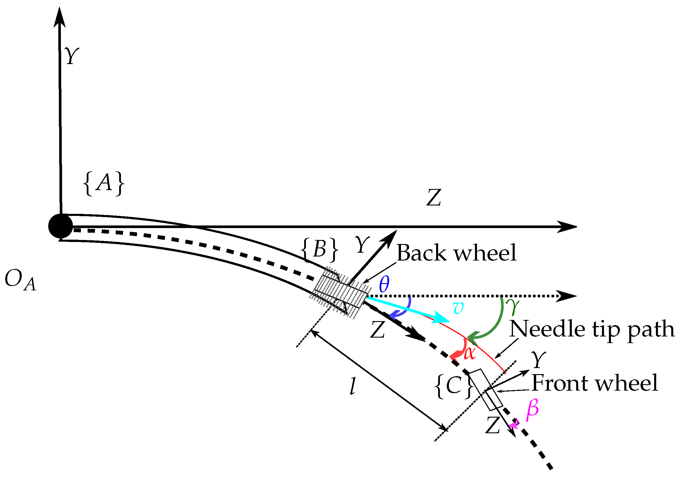
2.2. Extended Bicycle Model
The extended bicycle model [
8] considers a bicycle lying on the
plane as shown in
Figure 2 where labels
,
and
denote, respectively, the global fixed frame, the needle tip frame (back wheel) and the front wheel frame. The model consists of two wheels positioned at a fixed distance
l from each other with the front wheel oriented at a fixed angle
. The well-known bicycle model with front and back wheels is defined as
, parameterized by the
location of the back wheel and the angle of the bicycle body with respect to horizontal
. The constraints for the front and back wheels are formed by setting the sideways velocity of the wheels to zero. Using the Pfaffian constraints [
9], the following dynamical system is obtained:
with a
constant.
This model is modified in such a way that when the needle is moving forward into the tissue, lateral movements can happen on the back wheel due to tissue deformation. In this case, the final shape of the needle does not follow the tip path. This model, in contrast to the bicycle model in Equation (4), accounts for this phenomenon by considering an additional state,
. As for the unicycle model, we suppose that the needle path points toward the negative
y-axis starting from entry point
. As in the standard bicycle,
represents the
frame configuration which is the back wheel body frame. In contrast to the standard bicycle model, the needle tip configuration is
, where
is the angle between the
z-axis of the
frame and the needle tip velocity vector
. In practice,
describes a back wheel slippage phenomenon along the
y-axis of the
frame. If
defines needle tip velocity with respect to frame
,
defines the same quantity with respect to frame
, and the following relation holds:
As the needle bends toward the negative
y-axis, tissue deformation pulls the needle in the opposite direction, so
and
. The needle tip velocity vector
and the lateral slipping velocity
are defined as
where authors assume
as a quadratic function of
,
and
represent tissue-specific parameters related to its mechanical properties. Considering the definition of
as the slippage of the back wheel (Equation (
7)), it is clear that for non-zeros
and
, the needle path deviates from the constant curvature circular path corresponding to
. Using the definition of needle tip velocity
(
6a) and angle
(
5), angle
can be expressed as
Considering angle
(
5)–(
7), the time variation of angle
,
, is calculated as
Finally, the extended bicycle model [
8] can be written as
3. Method
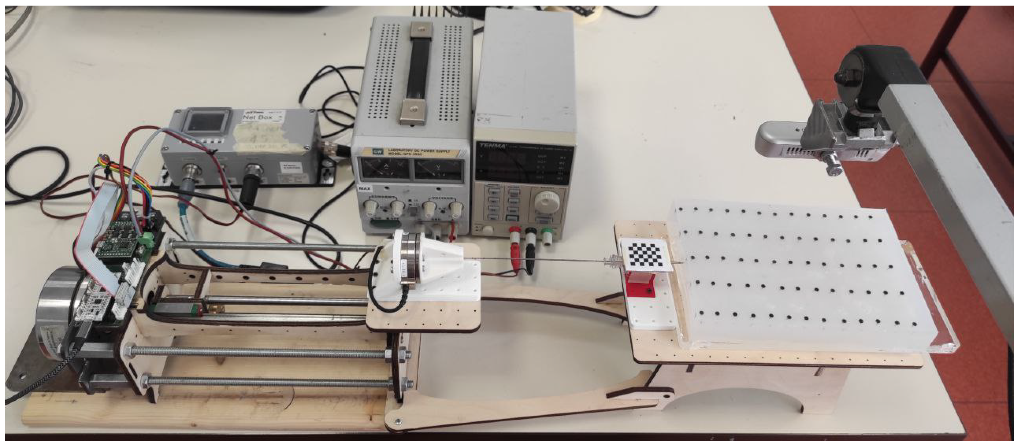
The experimental comparison is carried out with the setup shown in
Figure 3. It consists of a robotic system which performs the insertion with a bevelled tip needle. This system, described in
Section 3.4, includes a force sensor on the needle base and an external RGB-D camera. The insertions are performed on phantoms with different degrees of stiffness that emulate the prostate with different tumor levels defined by the Gleason score, which is a grading system for the progress of the tumor. Phantom preparation is described in
Section 3.5.
A fundamental step of our methodology is to identify the parameters of the unicycle and extended bicycle models to fit needle tip trajectory (
Section 3.1 and
Section 3.2). The trajectory is reconstructed using a vision algorithm (
Section 3.3) that identifies and tracks the needle tip throughout its insertion.
3.1. Unicycle Model Identification
This section introduces a methodology to estimate parameters
r and
for the unicycle model. Given needle tip coordinates
and
computed from the vision algorithm (see
Section 3.3), these are fitted to the unicycle circumference. The implicit equation of a circumference with a center in
and radius
r can be written as
To obtain a formulation suitable for least square regression in the form
, we rewrite (
11) as
where
and
. Then,
and
r can be easily found.
3.2. Extended Bicycle Model Identification
The authors of [
8] introduced a methodology to estimate the parameters of the extended bicycle model:
and
l in (
8) and
,
in (
7). From the needle tip trajectory
, computed from the vision algorithm in
Section 3.3, it is possible to measure the
angle as the orientation of needle tip velocity in the
frame:
where
,
, and
denote, respectively, the variations of needle tip deflection, insertion, and depth between two sample times. In this context, depth refers to the Euclidean distance in the
plane between two successive tip positions. Angle
is not directly measurable, but its time variation can be expressed in two different formulations, leading to
where (
14a) is obtained from (
8) substituting (
7) while (
14b) is calculated from (
10d) considering (
7). We combine (
14a) and (
14b) to obtain
which is a function of parameters and known quantities. Known quantities are
, (
13), its time variation
and the needle tip speed
v. Unknown parameters are
l,
,
, and
, and they can be identified by a non-linear least square regression algorithm as proposed by the authors [
8]. Unfortunately, the objective function presents several local minima and, to improve the results, the following constraints are imposed:
Even using such constraints, this methodology, as proposed by the authors [
8], is not always able to find an appropriate solution. For this reason, we use a genetic algorithm to minimize the residual error between the experimental data and the predicted ones.
3.3. Needle Recognition and Tracking
To track the needle tip position in each time frame, we used the semantic segmentation module based on the Generative Adversarial Network (GAN) model [
10]. Compared to the other models, this network has the advantage of requiring very few RGB samples representing the setup to obtain high-quality results. The GAN consists of two main components: a generator and a discriminator.
Generator: The generator takes an input image, processes it through a neural network, and produces an output image. It learns to create realistic and visually appealing results by mimicking the patterns, textures, and styles found in the training data. As training progresses, the generator becomes increasingly adept at generating images that are indistinguishable from real data.
Discriminator: The discriminator, on the other hand, acts as a critic. It tries to distinguish between real images from the training dataset and fake images generated by the generator. Through adversarial training, the discriminator becomes skilled at identifying flaws or inconsistencies in the generated images.
As training continues, the generator and the discriminator engage in a competitive process, with the generator constantly improving its ability to generate convincing output and the discriminator becoming better at discerning real from fake. This dynamic equilibrium ultimately results in the generator producing high-quality, pixel-to-pixel output that retains the essential characteristics of the input data.
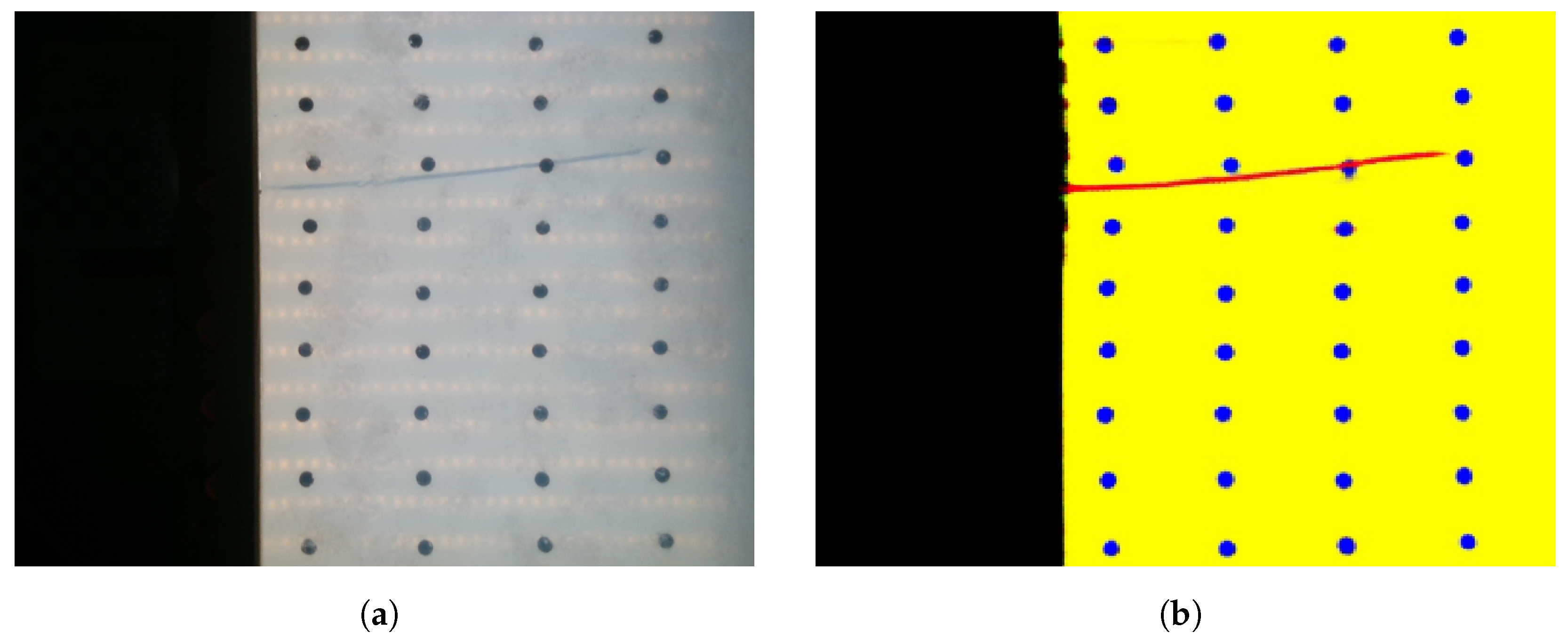
Figure 4 shows an example of segmentation of an image acquired from the realsense camera. The classes corresponding to objects in the scene are encoded following
Table 1.
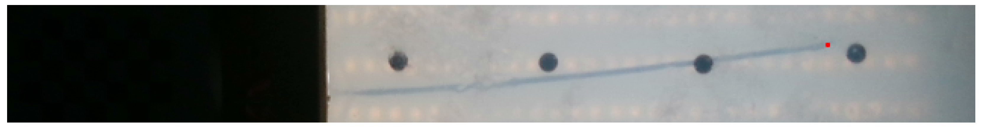
Once we obtained the segmented image, we defined the workspace by placing a chessboard over a 3D-printed support where the needle passes through. This allowed us to retrieve the pixel/millimeter ratio that is needed to have the needle position in the 3D metric space. Starting from the pose of the chessboard, we filtered out an area of interest around the needle path and created a bounding box in the semantic image, and then worked with a smaller image. Finally, we segmented the needle from the semantic image and then extracted the center point of the needle tip as shown in
Figure 5, which was used later for model estimation.
The coordinates of the needle tip, which are derived from the mask obtained through semantic segmentation for each frame, were individually subjected to a third-order polynomial fitting process over time-to-position data in order to mitigate measurement noise.
3.4. Experimental Setup
We design a robotic system to perform insertion experiments into tissues, with one degree of freedom (DoF) capable of translational motion along the needle’s principal axis. A mechanical drive system pushes the needle into the phantom using a direct drive motor (model EC90flat) and a worm gear system. The trajectory of the needle tip is reconstructed using an Intel RealSense d435 camera positioned approximately 20 cm from the surface of the phantom, operating at a rate of 30 Hz to capture the images fed into the vision algorithm. The use of transparent phantoms and a camera allows us to acquire the entire needle tip trajectory during the insertion with good accuracy, which is something ultrasound imaging cannot afford due to its noise.
The needle bevel tip is oriented so that the needle deflection plane is parallel to the imaging plane. In the experiments, a standard 18-gauge brachytherapy needle with a bevel angle of is used. The insertions are carried out at various constant velocities to a depth of 100 mm.
3.5. Phantom Design
In our comparative experiment, we evaluate four transparent phantoms with varying stiffness values (30, 50, 70, 100 kPa), covering the range associated with both benign and malign conditions of the prostate gland [
11,
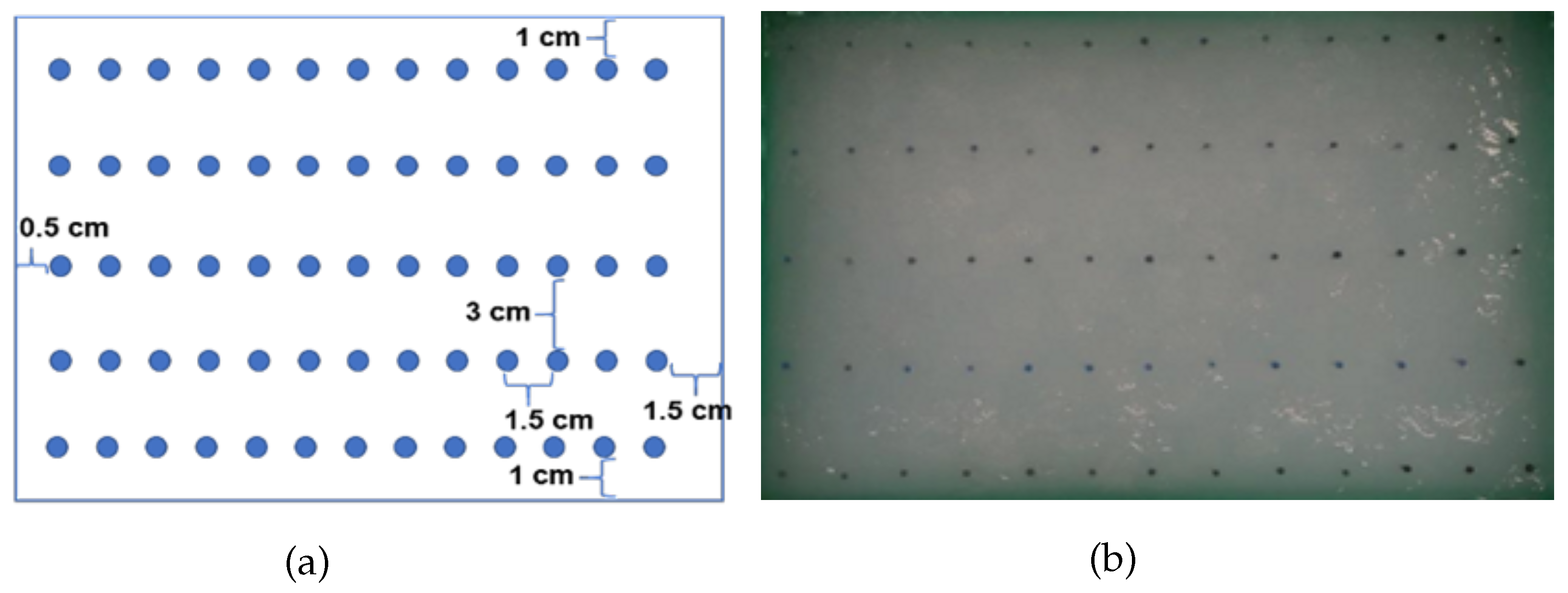
12]. Two-component silicone elastomers (SL 3358 A and SL 3358 B, KCC Corporation, Korea) were utilized in equal amounts for the preparation of the phantom. Silicone oil (G Line T100, KCC Corporation, Korea) in differing amounts (50, 55.5, 66.6) and 0.03 wt% cotton fibers were added to the silicone mixture to adjust the stiffness of the model and simulate the fibrous and muscular tissue of the prostate. The preparation of the first layer of the phantom body with fibers (2.5 cm height) was followed by the insertion of 65 pin markers (13 × 5 rows) positioned at the required locations (
Figure 6a). Subsequently, the final layer of the phantom (0.5 cm height) with fibers was produced by curing the silicone formulation that is equivalent to the bottom layer. Each layer was cured separately at 70 °C in an oven for 100 min (20 cm × 14 cm × 3 cm) (
Figure 6b).
3.6. Mechanical Characterization
Different formulations of the two-component silicone elastomers with silicone oil and cotton fiber supplements were prepared in dog bone shape according to the American Society for Testing and Materials International (ASTM) standards. The specimens were tested with 200 N force using the Universal Testing Machine (UTM) (Zwick/Roell), and an average of three tests were reported (
Figure 7).
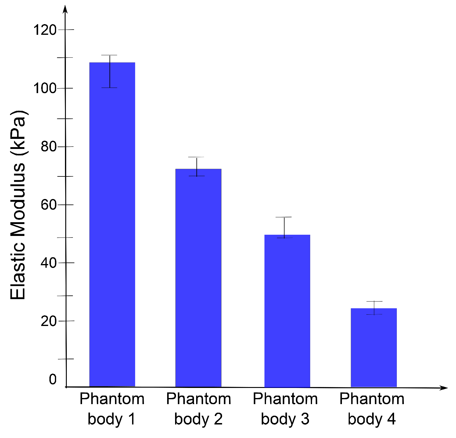
The degrees of stiffness were adjusted with the addition of silicone oil and supplementary materials (e.g., cotton fibers) to reach the highest resemblance to the reported values of the prostate tissue. The stiffness of the phantom body range was between 32.8 and 107 kPa (
Figure 8).
4. Experimental Results
Using the robotic setup, the needle is inserted to a depth of 100 mm considered to be the longest distance between the perineum and the apex of the prostate. Insertions are performed at two different velocities (10, 20 mm/s). For each stiffness and velocity pair, we perform four repetitions. We perform model identification procedures using data from the first three repetitions, and we use the fourth repetition to assess the prediction accuracy of the models. The unicycle model and the extended bicycle model are labeled, respectively, as
and
. Results in
Table 2 and
Table 3 show, respectively, the average final tip deflection
with the standard deviation of the final tip position
and the average tip error identification for unicycle model
and extended bicycle model
with their standard deviations
and
for every phantom’s stiffness and velocity pair.
Figure 9 shows examples of data from identification procedures related to phantoms with stiffness 30 kPa and 100 kPa at velocities 10
and 20
.
We estimate the parameters of the models by performing a least square identification for the unicycle model and using a genetic algorithm for the extended bicycle model as described in
Section 3.1 and
Section 3.2. To robustify the identification procedure, the estimated parameters are averaged considering data from the three insertions. To access the models’ accuracy, the simulated needle trajectory is compared to experimental data of the fourth repetition.
Results in
Table 4 show the maximum tip prediction error for unicycle model
and extended bicycle model
and their root-mean-squared errors (RMSEs)
and
for every phantom’s stiffness and velocity pair.
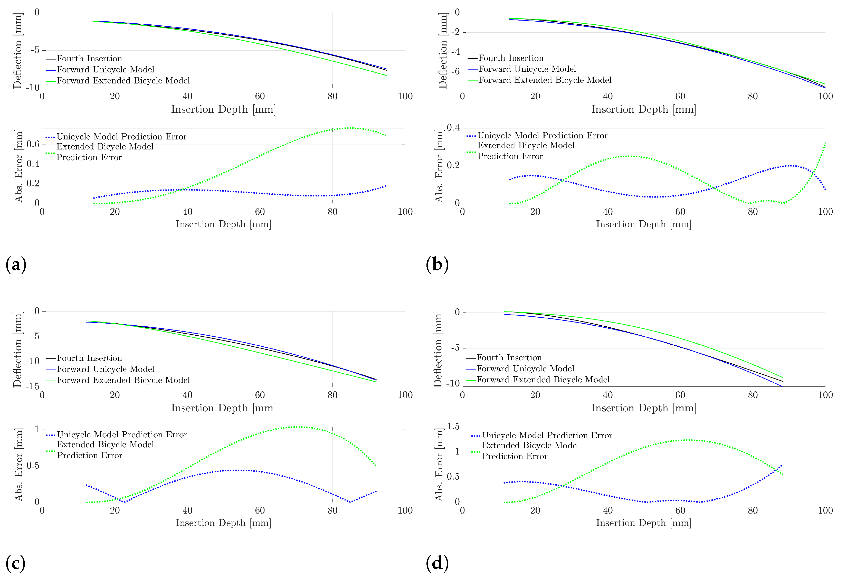
Figure 10 shows examples of data from prediction procedures related to phantoms with stiffness 30 kPa and 100 kPa at velocities 10
and 20
.
5. Discussion
From
Table 2, one can notice that insertions exhibit a notable final displacement, around 10% of their whole length, and this motivates the use of models for the prediction of needle deflection. From
Table 4, one can observe that both models are quite accurate in predicting the tip’s final position. In terms of RMSE, we achieved a tenth of a millimetre accuracy down to the millimetre (in the case of more rigid phantom insertions). The maximum errors were less than or equal to 0.75 mm for the unicycle model and less or equal to 2.07 mm for the extended bicycle model. In spite of its lower complexity, the unicycle model is more accurate than the extended bicycle model. Both in terms of RMSE and maximum error, the unicycle model is, on average, 2.5 times more accurate than the extended bicycle model. In any experimental scenario, the unicycle model generates smaller errors than the extended bicycle model (for each stiffness and velocity pair). For both models, higher errors in predicting the final needle tip deflection were obtained when the needle was pushed into the more rigid phantoms (70 and 100 kPa) at the highest velocity (20
). Since the unicycle model is a linear regression identification, it is faster and requires less computational effort than the extended bicycle model. We measured an average computation time of 0.7 ms for the unicycle model and 45 s (range 20–65 s, executed on Intel Core i7-6700HQ processor running four threads) for the extended bicycle model as a final remark.


 ,
, 


