
Rapid Tracking Satellite Servo Control for Three-Axis Satcom-on-the-Move Antenna

1
School of Power and Energy, Northwestern Polytechnical University, Xi’an 710072, China
2
Satpro M&C Tech Co., Ltd., Xi’an 710018, China
*
Author to whom correspondence should be addressed.
Aerospace 2024, 11(5), 345; https://0-doi-org.brum.beds.ac.uk/10.3390/aerospace11050345
Submission received: 27 February 2024
/
Revised: 19 April 2024
/
Accepted: 21 April 2024
/
Published: 26 April 2024
Abstract
:To overcome the possible gimbal lock problem of the dual-axis satcom-on-the-move (SOTM) antenna, a three-axis tracking satellite SOTM antenna structure appears. The three-axis SOTM antenna is realized by adding a roll axis to the azimuth axis and pitch axis in the dual-axis SOTM structure. There is coupling among the azimuth axis, pitch axis and roll axis in the mechanical structure of the three-axis SOTM antenna, which makes the kinematic modeling of the antenna difficult. This paper introduces a three-axis SOTM antenna kinematic modeling method based on the modified Denavit–Hartenberg (MDH) method, named the new modified Denavit–Hartenberg (NMDH) method. In order to meet the modeling requirements of the MDH method, the NMDH method adds virtual coordinate systems and auxiliary coordinate systems to the three-axis SOTM antenna and obtains the kinematic model of the three-axis SOTM antenna. During the motion of the carrier, the SOTM antenna needs to adjust the antenna pointing in real time according to the changes of the location and attitude of the moving carrier. Therefore, this paper designs a servo control system based on the active disturbance rejection controller (ADRC), introducing a smooth and continuous ADRC function to enhance the tracking speed of the servo control system and reduce the overshoot of the output response. Finally, system experiments were carried out with a 60 cm caliber three-axis SOTM antenna. The experiment results show that the proposed servo control method achieves higher antenna tracking satellite accuracy and better communication effects.
1. Introduction
Satcom-on-the-move (SOTM) plays an important role in satellite communications, which focuses on realizing real-time satellite communications during the motion of the carrier [1,2,3,4]. Through the SOTM system, carriers such as vehicles, ships and aircrafts can realize the continuous transmission of multimedia information such as data, voice, images and videos through satellites as relays during the movement, which can play an important role in many civil and military fields. Compared with the traditional communication method based on internet service provider (ISP) base stations, the communication of the SOTM system does not rely on fixed infrastructure, so it is not limited by the coverage area of ISP base stations and it has a wider range of applications and application scenarios, such as primitive forests, deserts and open seas, where ISP base stations cannot provide coverage. The SOTM system can easily realize Internet access and communication at a lower cost and the implementation method is more flexible.
The SOTM antenna usually adopts a dual-axis mechanical structure, including the azimuth axis and the pitch axis. The entire hemisphere can be scanned using these two axes. This mechanical structure has the advantages of simple design, low cost, robustness and compactness [5]. However, the dual-axis mechanical structure has an inherent shortcoming; that is, when the antenna pitch angle is 90°, the antenna pointing is perpendicular to the horizontal plane of the earth and the gimbal lock state is entered at this time [6]. In this case, when the carrier is moving, the antenna cannot continuously track the target satellite. The usual solution is to add a roll axis to the dual-axis SOTM antenna mechanical structure to form a three-axis SOTM antenna mechanical structure [7]. In engineering applications, system identification methods are often used for modeling, but it has the disadvantages of low applicability and poor portability. Especially for three-axis SOTM mechanical structure, a coupling relationship between the azimuth axis, the pitch axis and the roll axis increase the difficulty of modeling. For the three-axis SOTM mechanical structure, one method is to use the Newton–Euler method [8] for modeling, but the Euler equation established by this modeling method is more complicated, which makes the calculation and the processing difficulty, reducing the realization of the calculation of the kinematic relationship.
At present, traditional PID control still occupies a dominant position in the design and development of SOTM servo control systems [9,10,11]. This is because PID control has the advantages of low model relevance, simple controller structure, mature parameter adjustment methods, convenient design and development and no steady-state error [12,13,14,15,16,17,18]. However, in traditional PID control, the differential link D is a non-regular system and cannot be directly applied to system development. Therefore, in engineering applications, PI controllers are often used to replace PID controllers, or differential links with filters are used to replace traditional differential links. These schemes will reduce the performance of the PID controller or increase the complexity of the PID controller. In addition, there is a contradiction between the “rapidity” and “overshoot” of the PID controller [19,20,21,22]; that is, if the system output response is made to converge quickly, the system will have a large overshoot; if the system overshoot is reduced to a small value or even zero, the convergence speed of the system output response will be reduced. In the servo control system of the SOTM antenna, if the system output response converges slowly, it may result in the antenna failing to adjust to the required direction before changes in the carrier’s attitude and/or location occur, necessitating a readjustment of the antenna direction; if there is a significant overshoot, it could cause the SOTM antenna pointing to deviate from the target satellite. Both scenarios may have an impact on the tracking performance of the SOTM antenna on the satellite, potentially leading to the SOTM antenna losing track of the satellite.
The goal of this paper is to establish a three-axis SOTM antenna kinematic model that is simple to calculate and easy to implement and to design a servo controller that overcomes the contradiction between the rapidity and overshoot of the control system. The main contributions of this paper are: For the three-axis SOTM mechanical structure, a three-axis SOTM antenna kinematic model based on a new modified Denavit–Hartenberg (NMDH) method is introduced; a modified ADRC is introduced to improve the accuracy of the SOTM antenna pointing to the target satellite; a piecewise linear method is introduced to improve the engineering feasibility of the modified ADRC.
The remainder of this paper is organized as follows: Section 2 introduces the three-axis SOTM mechanical structure, introduces a NMDH method and thus obtains the kinematic model of the three-axis SOTM antenna and its inverse kinematic solution; Section 3 introduces an ADRC based on a smooth and continuous function as the controller of the SOTM servo control system and designs a function piecewise linear engineering implementation method; Section 4 is the experimental verification, which mainly verifies the scheme designed in this paper through experiments; Section 5 is the summary of the entire paper.
2. Kinematic Modeling of Three-Axis SOTM Antenna
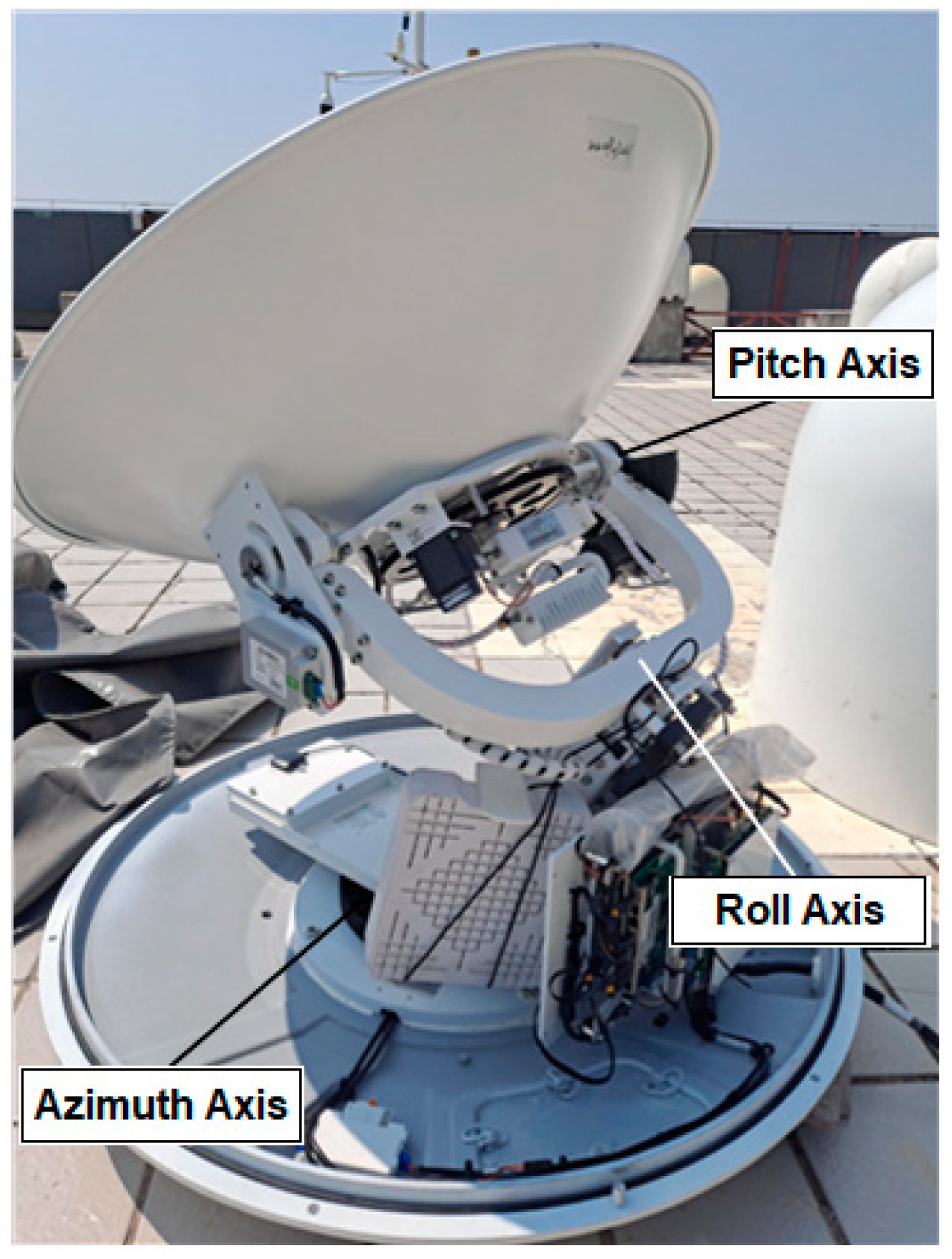
The three-axis SOTM antenna structure under study in this paper is illustrated in Figure 1. The entire system is installed on a fixed base, which is firmly attached to the carrier. Typically, bearings are employed to drive the base unit for rotational movement and mechanical linkage. Figure 2 displays a physical image of a three-axis SOTM antenna manufactured by SATPRO M&C Tech Co., Ltd. (located in Xi’an, China). The three-axis antenna system includes an azimuth sub-system, a roll sub-system and a pitch sub-system. Each of the three sub-systems has a rotating axis, which is used to adjust the antenna attitude, isolate the carrier disturbance and keep the antenna stable. Due to the limitation of the mechanical structure of the SOTM system, there is an angle less than 90° between the roll axis and the system base (generally 30°–35°) [23]. Brushless DC motors are usually used to drive the movement of each axis through gears or belt drives. The antenna used to transmit and receive satellite signals is installed on the pitch sub-system and moves with the pitch axis. The system uses a high-gain antenna to achieve wideband multimedia satellite communication. When the SOTM antenna tracking satellite error exceeds a certain range, it may interfere with adjacent satellites, causing the antenna to fail to transmit radio frequency signals. Therefore, the antenna pointing fluctuation must be kept within a sufficiently small range [24]. When measuring the antenna direction, a sensing system with sufficiently high precision and high sampling rate must be selected to quickly and accurately feed location and attitude information to the controller. The controller adjusts the antenna attitude by driving the motor, thereby ensuring that the antenna always points to the target satellite [25]. During continuous communication with the satellite, the servo system needs to continuously calculate the rotation angles of the three motors.
The three-axis SOTM antenna structure has three rotating axes, namely the azimuth axis, the pitch axis and the roll axis. In this section, we introduce an NMDH method based on the modified DH method [26,27,28,29] to establish the kinematic model of the three-axis SOTM antenna.
Based on the mechanical structure of the three-axis SOTM antenna, the antenna coordinate system configuration is obtained as shown in Figure 3. Among them, the coordinate system 0 is the reference coordinate system, which is firmly attached to the base. When the rotation angle of the azimuth axis is 0, the coordinate system 1 coincides with the reference coordinate system, the z-axis of the reference coordinate system coincides with the axis of the azimuth axis and represents the azimuth axis. Beta is the fixed angle between the roll axis and the base. The existence of this angle can improve the rigidity of the mechanical structure to improve the mechanical performance of the antenna, but it will increase the difficulty of modeling the antenna kinematic model. Since beta () is a fixed angle, it is difficult to directly use the modified DH method for system modeling. For this reason, a virtual coordinate system 2 is added in the coordinate system shown in Figure 3. In addition, due to the spatial relationship characteristics between and , and in Figure 3, the correct link length cannot be obtained along and respectively. Therefore, auxiliary coordinate system 3 and 5 are added in Figure 3 respectively. In Figure 3, the origins of the virtual coordinate system 2 and the auxiliary coordinate system 3 coincide, and the auxiliary coordinate system 5 and the origins of the coordinate system 6 coincide. In order to make Figure 3 clear, and are set in the figure to represent the two groups of coincident coordinate systems. Coordinate systems 4 and 6 represent the roll and pitch axes, with and denoting the rotation axes of the roll and pitch axes, respectively. This paper refers to the above method as the NMDH method.
Aiming at the global coordinate system configuration of the three-axis SOTM antenna mechanical structure shown in Figure 3, the D-H table of the three-axis SOTM antenna mechanical structure kinematic model is shown in Table 1.
According to the link parameters shown in the D-H table of the three-axis SOTM antenna system, the transformation matrices between each link are obtained as follows:
The total transformation matrix between the reference coordinate system 0 and the end pitch axis coordinate system 6 in the three-axis antenna system can be obtained from the above equations, then the forward kinematics model is calculated as follows:
Let , , , . Then,
where
,
,
,
,
,
,
,
,
,
,
,
,
is the direction matrix pointing the antenna towards the target satellite.
Next, the inverse kinematics solution of the three-axis SOTM antenna will be obtained, so as to obtain the real-time rotation angles of the azimuth axis, pitch axis and roll axis during the operation of the three-axis SOTM antenna. in Equation (7) can be calculated by the following equation:
where represents the rotation matrix from coordinate system to coordinate system .
The inverse kinematics solution of the three-axis SOTM antenna contains the following two cases:
(1) During the process of pointing the antenna towards the satellite in SOTM, the entire hemisphere can be scanned using azimuth and pitch axes. When the pitch angle of the tracking antenna is not 90°, the roll axis is fixed and is set to 0.
The inverse kinematic solution for the azimuth angle is obtained as:
The inverse kinematic solution for the pitch angle is:
or
Since the pitch angle must be between [0°, 90°], therefore should be within the range of [0°, 90°].
(2) When the pitch angle of the SOTM antenna reaches 90°, the antenna is in a locked state, and changing the azimuth axis cannot change the system’s orientation. In this case, the roll axis needs to be used, with the azimuth axis in a fixed state and is taken as the angle at which the antenna was last operated before entering the locked state; at this point, is known.
The inverse kinematic solution for the roll angle is obtained as:
According to Equation (12), it can be obtained that:
The inverse kinematic solution for the pitch angle is:
According to Equation (14), it can be obtained that:
3. Modified ADRC Servo Control Design
Currently, PID control is widely used in the servo control of SOTM antennas. After long-term development, the advantages of PID control, which are widely applicable and easy to design, have been widely recognized. PID control does not require an exact mathematical model of the controlled object; adjusting only three tunable parameters—the proportional constant, integral constant and differential constant, it can achieve good control effects and performance in most applications. However, PID control has some inherent disadvantages: it relies on an error-based design concept to eliminate errors, creating a certain time delay between system control action and disturbances. To swiftly suppress errors, higher control efforts are necessary, increasing the likelihood of overshoot, or even significant overshoot; when solely using the proportional part for control, the system may exhibit steady-state error. To eliminate this steady-state error, the integral element is introduced, but it may cause phase lag in the system and the integral element cannot effectively suppress specific disturbances. The mathematical model of the differential element is non-regular, making it a non-causal system that cannot be directly implemented. In digital PID controllers, the differential element is often replaced with a difference element, which reduces the efficiency of the differential element and subsequently affects the control effects of the PID controller. While combining PID and feedforward control can enhance the disturbance rejection capability of the controller, it is generally effective only for specific disturbances and necessitates a highly accurate system model, limiting its practical engineering applications.
A common scheme for servo control is to adopt a multi-loop design. The loops typically selected include the position loop, current loop, speed loop and others. For example, reference [30] proposed a design concept and method of adding an RC filtering network in the innermost loop to suppress high-frequency noise based on a multi-closed-loop design scheme. Each loop is designed using the PI control method, but the system’s uncertainties and nonlinearities were not considered. Building upon this foundation, reference [31,32] considered the nonlinear characteristics of the SOTM antenna system and introduced sliding mode control to enhance the stability of the control system and reduce steady-state errors based on the multi-loop control design concept. This method requires high modeling accuracy for the object and is unable to simultaneously meet the requirements of rapidity and overshoot. References [33,34] proposed a design scheme combining feedback control structure with feedforward control. By predicting the trend of system disturbances and providing feedforward compensation, it partially overcomes the shortcomings of traditional PID controllers in suppressing system disturbances. However, the premise is that the disturbances and the system model are known, so the disturbance rejection effect of feedforward control is not significant in complex disturbance environments. Reference [35] introduced feedback linearization methods and nonlinear system switching systems methods from modern control theory to enhance the robust stability of the control system. This method involves complex system design and requires high modeling accuracy. The aforementioned approaches cannot guarantee stable satellite communication in SOTM antenna system. Therefore, in the engineering field, PID control remains the mainstream design scheme for SOTM antenna servo control. However, there is the contradiction between rapidity and overshoot in PID control, and it does not address disturbances specifically but passively eliminates errors based on error. Therefore, using PID control SOTM antenna servo control systems cannot fully harness the efficiency of SOTM antenna systems.
For the SOTM antenna, when the aperture of parabolic antennas is small, the energy of the antenna beam relatively diverges, resulting in a wider antenna beam. Therefore, although it is easier to locate and track satellites with the small aperture of SOTM parabolic antennas, their communication quality is generally relatively poor. On the other hand, for large-aperture of parabolic antennas, due to the larger aperture size, the energy of the antenna beam is more concentrated, resulting in a narrower beam. While the narrow beam of large-aperture of SOTM parabolic antennas makes satellite acquisition and tracking more challenging, the concentrated antenna energy during steady-state satellite tracking with SOTM antennas enables large-aperture of parabolic antennas to achieve better communication quality. In the field of SOTM antenna applications, from the perspective of communication quality, if the installation size of the moving carrier allows, a system design using larger aperture antennas is generally preferred.
For larger-aperture SOTM antennas, if the SOTM antenna servo control system faces a contradiction between rapidity and overshoot, it may lead to the following issues: When the servo control system controls the antenna to quickly converge to the target direction, it may produce a large overshoot. At this point, once the SOTM antenna has aligned with the satellite, the presence of overshoot causes the antenna direction to keep adjusting, leading the antenna away from the optimal position. This deviation can result in reduced communication quality in the SOTM system and may even lead to interruptions in satellite communication if the antenna strays beyond the satellite beam coverage range. Additionally, because the carrier’s attitude and location may continuously change, the presence of the aforementioned overshoot further increases the difficulty of tracking satellites with the SOTM antenna. On the other hand, when the servo control system has a small overshoot or no overshoot, the antenna direction often requires a longer time to converge to the target direction. If the carrier’s location and altitude change little or not at all, the impact of this situation will be relatively minor. However, the SOTM system requires providing stable satellite communication services to users while the carrier is in motion. In a certain control cycle, due to the poor rapidity of the control system, when the servo control system has not yet adjusted the antenna direction to converge to the target direction, the carrier’s altitude and location may change, generating a new target direction for the SOTM antenna. This will cause the SOTM antenna to never converge to the ideal target direction, reducing the satellite communication quality of the SOTM system and even leading to interruptions in SOTM satellite communication. From the perspective of disturbance suppression, there are many sources of disturbance during the operation of the SOTM system, such as: environmental and atmospheric changes causing signal attenuation and multipath effects, changes in the motion carrier’s attitude and location and inherent vibrations, electromagnetic interference from the SOTM system itself, the moving carrier, or the surrounding environment, nonlinear characteristics introduced by gear backlash in servo transmission devices, production and installation errors between different batches of products, etc. The internal and external disturbances of the above-mentioned SOTM system generally have characteristics of being random, unpredictable and having no fixed features, making it difficult to effectively suppress these disturbances through conventional schemes.
Active Disturbance Rejection Control (ADRC) was proposed by Professor Jingqing Han of the Chinese Academy of Sciences in the 1990s, based on the principle of invariance. The core idea of ADRC is to treat the controlled object as a series integral type and to consider everything outside the series integral type object in the control system as the system’s equivalent total disturbance. By real-time estimation and elimination of this equivalent total disturbance, the control of complex controlled objects is simplified to that of a basic series integral type controlled object.
Figure 4 shows the block diagram of the ADRC structure. ADRC mainly consists of three major parts: the tracking differentiator (TD), the extended state observer (ESO) and the nonlinear state error feedback (NLSEF). The following sections will introduce these three parts of ADRC individually.
Tracking differentiator (TD):
For PID controllers, since the differential element is non-regular, an ideal differentiator is essentially physically unrealizable and can only be approximated by a differentiator with a filter or by a differencer. In the case of SOTM antenna systems, which use digital control technology, the differentiator is typically approximated by a differencer. Furthermore, due to the presence of significant random noise signals in SOTM antenna systems, random noise signals may be amplified, making the approximate differentiator unusable due to excessive deviation. Therefore, in the engineering application of SOTM antenna systems, PI controllers are commonly used. Due to the absence of the differential element, the dynamic performance of the system may be reduced. The main function of the tracking differentiator is to extract discontinuous or signal with random noise from the actual system as well as the differential of the signal. Additionally, it mitigates the contradiction between the rapidity and overshoot of the control system by arranging a transient process.
ADRC establishes an optimal synthesis function, based on which the Tracking Differentiator is designed to achieve rapid and synchronous extraction of the input signal and its differential, thereby reducing the amplification of random noise in the signal. Moreover, through the tracking differentiator, a smooth differential signal can be extracted. Simultaneously, by coordinating with the optimal synthesis function to arrange the transient process, it is possible to achieve rapid tracking of the input signal with minimal or even no overshoot.
The continuous tracking differentiator model is:
The corresponding discrete tracking differentiator model is:
In Equations (16) and (17), is the input signal, is the input signal extracted by the tracking differentiator, which is the tracking of the input signal, is the extracted differential signal and is the sampling period. function refers to the optimal synthesis function mentioned earlier and its expression is as follows:
In the function, is the response to the tracking speed of the input signal, known as the speed factor. while filters the noise carried by the signal, known as the filtering factor. Both the speed factor and the filtering factor are adjustable parameters. It is important to note that the filtering factor in the function and the sampling period in Equation (17) are not the same variable. The sampling period is determined at the beginning of system design and does not change, while the filtering factor is an adjustable parameter that can be modified according to changes in the control objective.
In the optimal synthesis function described by Equation (18), is the sign function and the specific expression of the function is shown in Equation (19):
Extended state observer (ESO):
In PID control, its ability to suppress system disturbances is relatively limited. When disturbance signals do not have specific characteristics and are unknown, PID struggles to effectively suppress all disturbances in the control system. In ADRC, the concepts of the nominal model and total disturbance are introduced. The nominal model is an expected model that deviates slightly from the system’s actual state, typically modeled as a series integral type. The difference between the actual model of the object and the desired nominal model is considered as the system’s internal disturbance, generally including inaccuracies in the model establishment and the unmodeled parts of the actual system contained within the established model. The starting point of ADRC in suppressing disturbances is to model the object as the desired nominal model, no longer distinguishing between internal and external disturbances, but rather treating them uniformly as the system’s total disturbance.
In the actual implementation process, an extended state observer was designed, which can observe the total disturbance of the system and expand it as a state to be output by the extended state observer. Leveraging the convergence of the extended state observer, it can accurately observe and extract the total disturbance of the system, making the observed total disturbance close to the true value. This design scheme does not differentiate between internal and external disturbances, reducing the complexity of disturbance analysis from a design perspective. The extended state observer is a focal point in the design of ADRC, addressing how to acquire system disturbances during the control process. It not only observes the state and the differential of state variables to differentiate from the output of the tracking differentiator, but also can expand the observed total internal and external disturbances of the system into a state. The extended state observer observes total disturbances without targeting disturbances with specific characteristics and does not require measurement through sensors to obtain a more accurate disturbance, simplifying the control system’s process of dealing with disturbances. Moreover, because the extended state observer can observe the total system disturbance in real-time accurately, appropriate compensation can be applied to enhance the system’s disturbance suppression performance significantly.
The continuous nonlinear extended state observer model is:
The corresponding discrete nonlinear extended state observer model is:
Wherein is the estimated value of the system state observed by the extended state observer, is the estimated value of the differential of the system state observed by the extended state observer, is the total disturbance of the system observed by the extended state observer, is the sampling period of the discrete system. In Equations (20) and (21), , , and are adjustable parameters of the controller. The specific mathematical description of the conventional function is:
Nonlinear state error feedback (NLSEF):
In PID control, the proportional, integral and differential elements are linearly weighted and summed. Studies show that this is not an efficient method for designing control systems. ADRC adopts a nonlinear feedback scheme and practical applications have shown that, compared to linear feedback, nonlinear feedback can enhance the control precision of the system and the feedback coefficients exhibit stronger adaptability.
In PID control, the integral term is used to eliminate steady-state error and suppress the adverse effects of disturbances on the system. When the system is subject to constant or persistent disturbances, the integral element can accumulate and gradually eliminate the resulting errors, ensuring that the system’s output can gradually return to the set point. This means that the integral element helps the control system better cope with persistent interference, thereby improving the system’s stability and robustness. However, in ADRC, because of the presence of the extended state observer, the total disturbance of the system can be estimated and the system can compensate for the adverse effects of the total disturbance. Therefore, in ADRC, the integration of the error signal is usually not used and only the error signal and its differential are needed. By using the input signal and its differential extracted by the tracking differentiator and the estimated values of the system’s state variables and their differential obtained through the extended state observer, the error signal and its differential can be obtained by taking the difference.
Nonlinear state error feedback generally has two forms of expression, one of which is:
Another form of expression is:
In Equations (23) and (24), is the error signal, is the differential of the error signal and , , , , , and are adjustable parameters of the controller.
In ADRC, the performance of the extended state observer significantly impacts the control effect of the control system. The control system needs to compensate for the total disturbance, which is observed and estimated by the extended state observer. The function, derived from engineering practice through fitting, does not have a unique form. In ADRC, the function is a continuous function, but it has non-differentiable points, namely at and in Equation (22), where the left and right derivatives of the function are not equal. These points are cusp points, indicating that it is a continuous but non-smooth function. Studies have shown that the continuous smoothness of the function significantly affects the control effect of ADRC [36]. Thus, the function may adversely affect the control system, there is a need to develop a new function [37,38,39]. Therefore, this paper introduces a new function as presented in Equation (25):
where
In this paper, the function described by Equation (25) is referred to as the improved function, whereas the ADRC based on this improved function is referred to as the modified ADRC. Next, we verify whether the improved function is a smooth continuous function. Firstly, we verify its continuity, taking the point as an example for analysis. Let , , then:
The following can be obtained:
This implies that the improved function is continuous at the point . Using the same method, it can be concluded that the improved function is also continuous at the point .
Secondly, we verify the smoothness of the improved function, primarily by checking whether the left and right derivatives of the function at points and are equal.
It can be obtained that,
Given that the left and right derivatives of the improved function are equal at , it indicates that the improved function is smooth at . Applying the same method, it is possible to deduce that the improved function is also smooth at .
Summarizing the above process, the improved function is a smooth and continuous function at both and .
Next, we verify the symmetry of the improved function.
When , it can be easily derived,
When ,
When ,
In summary, the improved function is centrosymmetric about the origin.
As shown in Figure 5, it is a comparison of the curves between the conventional function and the improved function. In the figure, taking , it can be observed that at two separate points and , the conventional function is continuous but not smooth, whereas the improved function is both continuous and smooth. Furthermore, both the conventional function and the improved function are symmetric about the origin, which is consistent with the theoretical deductions previously discussed.
Although the improved function is a smooth and continuous function, it is much more complex than the conventional function when , including nonlinear elements such as trigonometric functions. Likewise, when , the improved function involves nonlinear elements such as exponential calculations. The equation for the improved function is known and from a mathematical standpoint, its implementation is relatively straightforward and does not require further discussion. However, from the perspective of implementation in SOTM systems, due to the presence of the aforementioned complex calculations, microprocessors need to perform repeated floating-point multiplications, divisions and other operations when processing these calculations, which typically require more clock cycles to complete, consuming more computing resources and time. Especially for low-cost, low-power microprocessors, this requires more computational resources and time. Although the performance of microprocessors has improved, enabling high-end microprocessors to feature specialized hardware or instruction sets optimized for these complex calculations to enhance performance and computational efficiency. For most microprocessors, exponential and trigonometric calculations require substantial computing resources and time, presenting a significant challenge for microprocessors serving as controllers. Based on this, this paper proposes a piecewise linearization method for the improved function by approximating segmented straight lines to simplify calculations, thereby reducing the processing difficulty for microprocessors, enhancing their computational efficiency and decreasing the consumption of computational resources and time on the microprocessor.
A schematic diagram of the piecewise linearization method for the improved function is shown in Figure 6. It should be noted that the method of selecting points described in this paper is not the only one. It can be adjusted according to different parameters of the improved function and verified by experiments or simulations. Figure 6 provides only one example. In Figure 6, several points, namely , , , , are selected on the curve of the function, with line segments , , , connecting two adjacent points. Since the coordinates of points , , , are known, the equations for line segments , , , can be easily obtained:
From Figure 6, it can be seen that the line formed by connecting segments , , , closely approximates the curve of the improved function. For the aforementioned piecewise linearization method, it is sufficient to store the parameters of each line and the coordinates of each point locally in the microprocessor to easily compute the improved function. Since the expression for each segment is a linear function, it can be calculated quickly and efficiently to obtain the value of the improved function by microprocessors with hardware floating-point capabilities. This method consumes less computing resources and time for microprocessors. Additionally, as mentioned earlier, since the improved function is symmetrical about the origin, it is only necessary to select points and connect them with line segments either after or before the point of the improved function. The other half can be easily obtained by utilizing the central symmetry property of the improved function, which can reduce the consumption of the microprocessor’s local storage resources to some extent.
4. Experiment Analysis
This section verifies the effectiveness of the proposed schemes through experimental methods. The experimental equipment utilizes a 60 cm caliber three-axis SOTM antenna. In this section, the ADRC based on the conventional function is referred to as conventional ADRC, while the ADRC based on the improved function is referred to as modified ADRC.
4.1. Experiment Setting
Experiment Address: SATPRO M&C Tech Co., Ltd., Weiyang District, Xi’an, China
Experiment Date: 17 November 2023
Experiment Weather: Sunny, −3 °C
Coordinates of the Swing Platform: 108.8479° E, 34.3679° N
Target Communication Satellite: YATAI 6D Geosynchronous Satellite
Antenna Manufacture: SATPRO M&C Tech Co., Ltd. (Xi’an, China)
Antenna Working Band: Ku Band
Antenna Receiving Frequency: 10.7–12.75 GHz
Antenna Transmitting Frequency: 13.75–14.5 GHz
Azimuth range of the Swing Platform: −15°–15°
Pitch range of the Swing Platform: −15°–15°
Roll range of the Swing Platform: −15°–15°
Antenna Azimuth Scanning Range: 0°–360°
Antenna Pitch Scanning Range: 0°–90°
Antenna Roll Scanning Range: −15°–15°
The experimental site environment is shown in Figure 7.
4.2. Experiment Results
Experiments were conducted using both conventional ADRC and modified ADRC for comparison, with each experiment lasting about 30 min.
The azimuth orientation of the SOTM antenna when using conventional ADRC and modified ADRC is illustrated in Figure 8. To clarify the curve details and improve the readability of the graphical information, data spanning a continuous 200-s are selected for plotting. From Figure 8, it can be observed that, compared to conventional ADRC, the fluctuation in the azimuth orientation of the SOTM antenna is smaller with the modified ADRC proposed in this paper, indicating that the modified ADRC enables a more precise azimuth orientation of the SOTM antenna.
The pitch orientation of the SOTM antenna when using conventional ADRC and modified ADRC is illustrated in Figure 9. Similarly, to clarify the curve details and improve the readability of the graphical information, data spanning a continuous 200-s are selected for plotting. From Figure 9, it can be observed that, compared to conventional ADRC, the fluctuation in the pitch orientation of the SOTM antenna is smaller with the modified ADRC proposed in this paper, indicating that the modified ADRC enables a more precise pitch orientation of the SOTM antenna.
Integrating the experiment results from both azimuth and pitch orientation, it can be concluded that, relative to conventional ADRC, the use of the modified ADRC introduced in this paper results in better tracking performance of the SOTM antenna towards the target communication satellite.
As shown in Table 2, the statistical characteristics of pointing data for SOTM system throughout the entire experiment are presented. In the table, the units for the maximum, minimum, average and range of both azimuth and pitch angles are degrees, while the variance is dimensionless.
From Table 2, it can be seen that compared to conventional ADRC, the modified ADRC introduced in this paper has reduced the fluctuation range of the azimuth angle by 22.97% and the pitch angle by 8.47%. This indicates that using the modified ADRC leads to higher precision in the SOTM antenna towards satellite tracking.
Next, the real-time automatic gain control (AGC) level, real-time signal to noise ratio (SNR) and signal quality are integrated to verify the communication performance of the SOTM system during the experiment.
The AGC levels of the SOTM antenna when using conventional ADRC and modified ADRC are illustrated in Figure 10. Similarly, to clarify the curve details and improve the readability of the graphical information, data spanning a continuous 200-s are selected for plotting. From Figure 10, it can be observed that, compared to conventional ADRC, the AGC levels are higher with modified ADRC proposed in this paper. This indicates that the communication performance of the SOTM antenna is better with the modified ADRC.
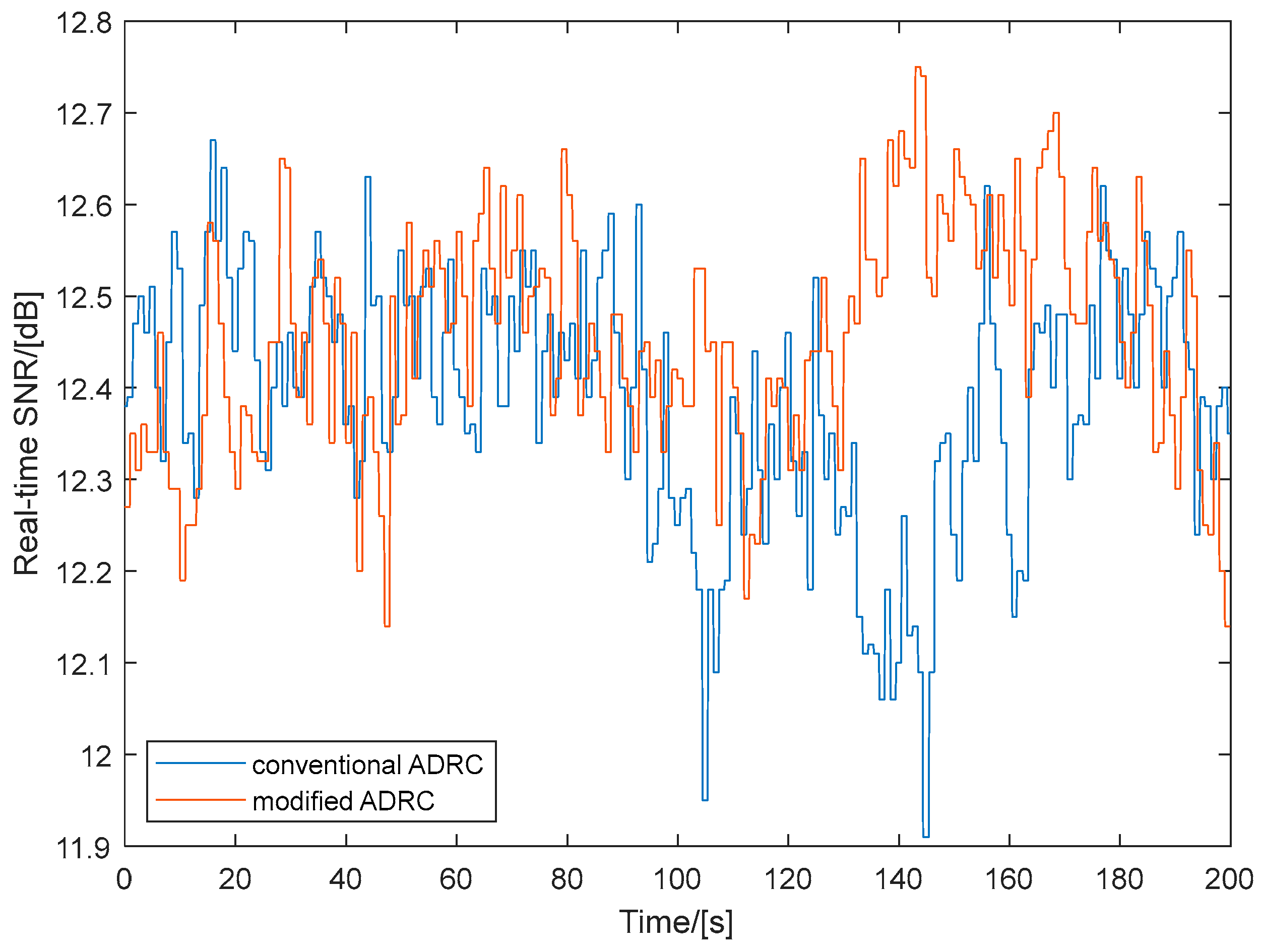
The SNR of the SOTM antenna when using conventional ADRC and modified ADRC is illustrated in Figure 11. Similarly, to clarify the curve details and improve the readability of the graphical information, data spanning a continuous 200-s are selected for plotting. From Figure 11, it can be observed that, compared to conventional ADRC, the SNR values are higher with the modified ADRC proposed in this paper. This indicates that the communication performance of the SOTM antenna is better with the modified ADRC.
The signal quality of the SOTM antenna when using conventional ADRC and modified ADRC is illustrated in Figure 12. Similarly, to clarify the curve details and improve the readability of the graphical information, data spanning a continuous 200-s are selected for plotting. From Figure 12, it can be observed that, compared to conventional ADRC, the signal quality values are higher with the modified ADRC proposed in this paper. This indicates that the communication performance of the SOTM antenna is better with the modified ADRC.
As shown in Table 3, the statistical characteristics of the communication-related data for SOTM system throughout the entire experiment are presented. In the table, the expected unit for SNR is dB, the unit for AGC level is V and the unit for signal quality (represented by SQ in Table 3) is %, the variance for all is dimensionless.
As shown in Table 3, throughout the entire experiment, compared to conventional ADRC, the modified ADRC introduced in this paper resulted in enhancements in the AGC level, SNR and signal quality of the SOTM system. At the same time, the variance of these three indicators decreased, indicating that the use of modified ADRC improves the communication performance of the SOTM system and makes the communication more stable. It should be noted that, due to the relatively small range of AGC level, SNR and signal quality in the normal running of SOTM system, there will not be a significant difference in the AGC level, SNR and signal quality between the two control schemes in Table 3.
Finally, tests were conducted on the communication latency of SOTM system using conventional ADRC and modified ADRC separately to verify the effectiveness of the proposed modified ADRC control scheme. These tests were carried out using the operating system’s “ping” command, with the target address set as China Telecom’s “114.114.114.114”. The testing sites are shown in Figure 13.
During the communication latency testing process, the statistical data for communication latency using conventional ADRC and modified ADRC methods are shown in Table 4, where the unit of communication latency is ms.
Based on the data in Table 4, it can be observed that during the experimental process, in comparison to conventional ADRC, when the modified ADRC proposed in this paper is utilized, the communication latency of the SOTM system is reduced, with lower latency fluctuations (i.e., smaller variance), implying that employing the modified ADRC can decrease the communication latency of the SOTM system, making communication more stable.
Integrating all the experiment results, it can be concluded that compared to conventional ADRC, the use of the modified ADRC introduced in this paper results in better precision in tracking target communication satellites of the SOTM antenna, as well as superior communication performance and stability of the SOTM system. This demonstrates that the scheme proposed in this paper is suitable for application in the development of SOTM systems.
5. Conclusions
For the mechanical structure of a three-axis SOTM antenna, this paper introduces a kinematic modeling method for the three-axis SOTM antenna based on a new modified Denavit–Hartenberg method. To meet the modeling requirements of the MDH method, virtual and auxiliary coordinate systems are designed and added to the global coordinate of the three-axis SOTM antenna to obtain its kinematic model. The SOTM antenna needs to adjust its pointing direction in real time according to the changes in the location and attitude of the moving carrier. Therefore, this paper designs a servo control system based on ADRC and introduces a smooth and continuous function of ADRC to enhance the tracking speed of the servo control system and reduce the overshoot of the output response. In addition, aiming at the drawback of the complex calculation of the improved function, a piecewise linear approximation method is designed, which transforms the complex nonlinear function operation into a simple linear function operation, thereby reducing the engineering implementation difficulty of the modified ADRC. Finally, the designed scheme was validated through experiments. The experiment results show that, compared to conventional ADRC, the proposed servo control method based on modified ADRC achieved higher antenna tracking satellite accuracy and improved communication performance.
Author Contributions
Conceptualization, J.R. and X.J.; methodology, J.R., L.H., S.S. and Y.W.; software, J.R. and J.L.; validation, X.J., S.S., J.L. and Y.W.; formal analysis, J.R.; investigation, J.R. and J.L.; resources, L.H.; data curation, X.J. and L.H.; writing—original draft preparation, J.R., X.J. and L.H.; writing—review and editing, J.R., X.J., S.S., Y.W. and J.L.; supervision, X.J. and Y.W.; project administration, X.J. and L.H.; funding acquisition, X.J. All authors have read and agreed to the published version of the manuscript.
Funding
This research was funded by Qin Chuang Yuan Construction of Two Chain Integration Special Project, grant number 23LLRH0006.
Data Availability Statement
The data used to support the findings of this study are included within the article.
Conflicts of Interest
Authors Lei Han and Xiaoxiang Ji were employed by the Satpro M&C Tech Co., Ltd. The remaining authors declare that the research was conducted in the absence of any commercial or financial relationships that could be construed as potential conflict of Interest.
Abbreviations
The following abbreviations are used in this manuscript:
| SOTM | Satcom-on-the-Move |
| DH | Denavit-Hartenberg |
| MDH | Modified DH |
| NMDH | New Modified DH |
| ADRC | Active Disturbance Rejection Controller |
| AGC | Automatic Gain Control |
| SNR | Signal to Noise Ratio |
| SQ | Signal Quality |
References
- Mohamed, H.; Moustafa, E.; Roshdy, A.; Mohamed, Z.; Mohamed, G. SATCOM on-the-Move Antenna Tracking Survey. In Proceedings of the 2021 9th International Japan-Africa Conference on Electronics, Communications, and Computations (JAC-ECC), Alexandria, Egypt, 13–14 December 2021. [Google Scholar]
- Han, L.; Li, G.; Ren, J.; Ji, X. Synthetic Deviation Correction Method for Tracking Satellite of the SOTM Antenna on High Maneuveribility Carriers. Electronics 2022, 11, 3732. [Google Scholar] [CrossRef]
- Yuan, D.; Qin, Y.; Wu, Z.; Shen, X. A Robust Multi-State Constraint Optimization-Based Orientation Estimation System for Satcom-on-the-Move. IEEE Trans. Instrum. Meas. 2021, 70, 5503314. [Google Scholar] [CrossRef]
- Baghdadi, H.; Royo, G.; Bel, I.; Cortes, F.; Celma, S. Compact 2 × 2 Circularly Polarized Aperture-Coupled Antenna Array for Ka-Band Satcom-on-the-Move Applications. Electronics 2021, 10, 1621. [Google Scholar] [CrossRef]
- Michal, B.; Jan, N.; Tomas, S. Design of an Antenna Pedestal Stabilization Controller Based on Cascade Topology. In Proceedings of the Mechatronics 2019: Recent Advances Towards Industry 4.0, Warsaw, Poland, 16–18 September 2019. [Google Scholar]
- Laetitia, T.; Minh, P.; Paolo, M.; Elliot, B. Rapid Transfer Alignment for Large and Time-Varying Attitude Misalignment Angles. IEEE Control Syst. Lett. 2023, 7, 1981–1986. [Google Scholar]
- Han, L.; Ren, J.; Ji, X.; Li, G. Multi-Beam Satellite Seeking and Acquisition Method for Satcom-on-the-Move Array Antenna on a High Maneuverability Carrier. Appl. Sci. 2023, 13, 11803. [Google Scholar] [CrossRef]
- Djizi, H.; Zahzouh, Z.; Bouzaouit, A. Quadcopter Prototype Stability Assessment with Pid Control and Euler-Lagrange Approach. Sci. Bull. Electr. Eng. Fac. 2023, 1, 15–20. [Google Scholar]
- Yang, X.; Huang, Q.; Jing, S.; Zhang, M.; Zuo, Z.; Wang, S. Servo System Control of Satcom on the Move Based on Improved ADRC Controller. Energy Rep. 2022, 8, 1062–1070. [Google Scholar] [CrossRef]
- Xue, X.; Zheng, J.; Yuan, D. Adaptive Control of Servo Motor in “SOTM”. In Proceedings of the 2018 3rd International Conference on Control, Automation and Artificial Intelligence (CAAI 2018), Beijing, China, 26–27 August 2018. [Google Scholar]
- Wang, Y.; Zhang, C.; Zuo, Z. Anti-Windup Active Disturbance Rejection Control and Its Application to Antenna Servo Systems. In Proceedings of the 2019 Chinese Control Conference (CCC), Guangzhou, China, 27–30 July 2019. [Google Scholar]
- Balamurugan, S.; Umarani, A. Study of Discrete PID Controller for DC Motor Speed Control Using MATLAB. In Proceedings of the 2020 International Conference on Computing and Information Technology (ICCIT-1441), Tabuk, Saudi Arabia, 9–10 September 2020. [Google Scholar]
- Tigo, W.; Subiyanto; Sutarno. Simulation Model of Speed Control DC Motor Using Fractional Order PID Control. In Proceedings of the 8th Engineering International Conference 2019, Semarang, Indonesia, 16 August 2019. [Google Scholar]
- George, T.; Ganesan, V. Optimal Tuning of PID Controller in Time Delay System: A Review on Various Optimization Techniques. Chem. Prod. Process Model. 2022, 17, 1–28. [Google Scholar] [CrossRef]
- Hari, M.; Musyaffa, A.; Agus, R.; Feri, A. Fuzzy-PID in BLDC Motor Speed Control Using MATLAB/Simulink. J. Robot. Control 2022, 3, 8–13. [Google Scholar]
- Oluwasegun, S.; Kayode, A.; Folasade, D. The Dilemma of PID Tuning. Annu. Rev. Control 2021, 52, 65–74. [Google Scholar]
- Liqaa, M. Speed Control for Servo DC Motor with Different Tuning PID Controller with Labview. J. Mech. Eng. Res. Dev. 2021, 44, 294–303. [Google Scholar]
- Damir, V.; Mikulas, H. High-Order Filtered PID Controller Tuning Based on Magnitude Optimum. Mathematics 2021, 9, 1340. [Google Scholar] [CrossRef]
- Yang, L.; Jing, X.; Shuang, M.; Qiang, H.; Yue, S. A Comparative Study of the First Order Linear ADRC and PI Controller in the Speed Control System of Permanent Magnet Synchronous Motor. In Proceedings of the 2020 IEEE 9th Data Driven Control and Learning Systems Conference (DDCLS), Liuzhou, China, 20–22 November 2020. [Google Scholar]
- Liang, S.; Guo, M.; Tian, Y.; Le, J.; Song, W. Research on Intelligent Active Disturbance Rejection Control Algorithm for Shock Train Leading Edge of Dual-Mode Scramjet. Phys. Fluids 2024, 36, 015103. [Google Scholar] [CrossRef]
- Wang, Z.; Xiong, H. Research on ADRC Based on Speed Loop Control of Permanent Magnet Synchronous Motor. In Proceedings of the 3rd International Conference on Electrical Engineering and Mechatronics Technology (ICEEMT), Nanjing, China, 21–23 July 2023. [Google Scholar]
- Han, J.; Guo, J.; Zhao, Z.; Ma, Z.; Liu, Y.; Zou, S. Orientation Control and Target Tracking for Bionic Robotic Fish Based on ADRC. In Proceedings of the 2023 42nd Chinese Control Conference (CCC), Tianjin, China, 24–26 July 2023. [Google Scholar]
- James, D. Control Systems for Mobile Satcom Antennas. IEEE Control. Syst. Mag. 2008, 28, 86–101. [Google Scholar]
- Oguz, H.; Mehmet, E. Neural Network Control of a SOTM Antenna. In Proceedings of the 2023 9th International Conference on Control, Decision and Information Technologies (CoDIT), Rome, Italy, 3–6 July 2023. [Google Scholar]
- Michal, B.; Tomas, S.; Jan, N.; Mustafa, C.; Oguz, H.; Robert, G. Estimation of Maximum Signal Strength for Satellite Tracking Based on the Extended Kalman Filter. Adv. Mil. Technol. 2023, 18, 87–99. [Google Scholar]
- Xu, C.; Zhu, H.; Zhu, H.; Wang, J.; Zhao, Q. Improved RRT* Algorithm for Automatic Charging Robot Obstacle Avoidance Path Planning in Complex Environments. CMES-Comp. Model. Eng. 2023, 137, 2567–2591. [Google Scholar] [CrossRef]
- Cozmin, C.; Mario, I.; Ionut, G.; Cristina, P. The Importance of Embedding a General Forward Kinematic Model for Industrial Robot with Serial Architecture in Order to Compensate for Positioning Errors. Mathematics 2023, 11, 2306. [Google Scholar] [CrossRef]
- Oguz, H.; Mustafa, C.; Ugur, T. Kinematics and Tracking Control of a Four Axis Antenna for Satcom on the Move. In Proceedings of the 2018 International Power Electronics Conference (IPEC-Niigata 2018—ECCE Asia), Niigata, Japan, 20–24 May 2018. [Google Scholar]
- Chen, Y.; Chen, L.; Ding, J.; Liu, Y. Research on Real-Time Obstacle Avoidance Motion Planning of Industrial Robotic Arm Based on Artificial Potential Field Method in Joint Space. Appl. Sci. 2023, 13, 6973. [Google Scholar] [CrossRef]
- Li, F.; Xia, Q.; Qi, Z. Analysis and Design of Three Loop Radar Servo System for Air Defense Missile. In Proceedings of the 2011 Third International Conference on Measuring Technology and Mechatronics Automation, Shanghai, China, 6–7 January 2011. [Google Scholar]
- Fujimoto, Y.; Kawamura, A. Robust Servo-system Based on Two-degree-of-freedom Control with Sliding Mode. IEEE Trans. Ind. Electron. 1995, 42, 272–280. [Google Scholar] [CrossRef]
- Suzumura, A.; Fujimoto, Y.; Murakami, T.; Oboe, R. A General Framework for Designing SISO-Based Motion Controller with Multiple Sensor Feedback. IEEE Trans. Ind. Electron. 2016, 63, 7607–7620. [Google Scholar] [CrossRef]
- Liu, X.; Huang, Q.; Chen, Y.; Li, J. Nonlinear Modeling and Optimal Controller Design for Radar Servo System. In Proceedings of the 2009 Third International Symposium on Intelligent Information Technology Application, Nanchang, China, 21–22 November 2009. [Google Scholar]
- Peng, C.; Wang, Y. Identification of State Space Model for Radar Servo System. In Proceedings of the 32nd Chinese Control Conference, Xi’an, China, 26–28 July 2013. [Google Scholar]
- Mario, G.; Trupti, R.; Bhal, J. Advanced Nonlinear Robust Controller Design for High-Performance Servo-Systems in Large Radar Antennas. In Proceedings of the 2011 IEEE National Aerospace and Electronics Conference (NAECON), Dayton, OH, USA, 20–22 July 2011. [Google Scholar]
- Seyed, M.; Seyed, S.; Hamed, M. Speed Control of a DFIG-Based Wind Turbine Using a New Generation of ADRC. Int. J. Green Energy 2023, 20, 1669–1698. [Google Scholar]
- Yue, L.; Wang, Y.; Xiao, B.; Wang, Y.; Lin, J. Improved Active Disturbance Rejection Speed Control for Autonomous Driving of High-Speed Train Based on Feedforward Compensation. Sci. Prog.-UK 2023, 106, 368504231208505. [Google Scholar] [CrossRef] [PubMed]
- Hua, Z.; Ruan, H.; Tu, D.; Zhang, X.; Zhang, K. Research on Motion Control of Underwater Robot Based on Improved Active Disturbance Rejection Control. In Proceeding of the International Conference on Intelligent Robotics and Applications, Hangzhou, China, 5–7 July 2023. [Google Scholar]
- Liu, B.; Li, M.; Yang, J. Attitude Control of Quadrotor Aircraft Based on Improved ADRC. Command Control Simul. 2021, 43, 98–102. [Google Scholar]
Figure 1.
Structure of the three-axis SOTM antenna.

Figure 2.
Three-axis SOTM antenna manufactured by SATPRO (located in Xi’an, China).

Figure 3.
Parameters and coordinate system configuration of three-axis SOTM antenna.

Figure 4.
Structure of the ADRC.

Figure 5.
Conventional function and the improved function.

Figure 6.
A schematic diagram of the piecewise linearization method for the improved function.

Figure 7.
Experiment site.

Figure 8.
The azimuth angles of SOTM antenna when using conventional ADRC and modified ADRC.

Figure 9.
The pitch angles of SOTM antenna using conventional ADRC and modified ADRC.

Figure 10.
The real-time AGC of SOTM antenna when using conventional ADRC and modified ADRC.

Figure 11.
The real-time SNR of SOTM antenna when using conventional ADRC and modified ADRC.

Figure 12.
The real-time signal quality of SOTM antenna when using conventional ADRC and modified ADRC.
Figure 12.
The real-time signal quality of SOTM antenna when using conventional ADRC and modified ADRC.

Figure 13.
Communication latency testing: (a) Conventional ADRC; (b) Modified ADRC.


Table 1.
D-H table of the three-axis SOTM antenna.
| 1 | ||||
| 2 | ||||
| 3 | ||||
| 4 | ||||
| 5 | ||||
| 6 |
Table 2.
Statistical characteristics of antenna pointing throughout the entire experimental process.
Table 2.
Statistical characteristics of antenna pointing throughout the entire experimental process.
| Conventional ADRC | Modified ADRC | |||
|---|---|---|---|---|
| Azimuth Angle | Pitch Angle | Azimuth Angle | Pitch Angle | |
| Max Value | 141.89 | 43.08 | 141.71 | 43.12 |
| Min Value | 140.98 | 42.44 | 140.97 | 42.53 |
| Mean Value | 141.35 | 42.78 | 141.36 | 42.81 |
| Range | 0.91 | 0.64 | 0.74 | 0.59 |
| Variance | 3.49 × 10⁻² | 2.12 × 10⁻² | 3.12 × 10⁻² | 2.05 × 10⁻² |
Table 3.
Statistical characteristics of the communication-related data throughout the entire experiment.
Table 3.
Statistical characteristics of the communication-related data throughout the entire experiment.
| Conventional ADRC | Modified ADRC | |||||
|---|---|---|---|---|---|---|
| AGC | SNR | SQ | AGC | SNR | SQ | |
| Mean Value | 2.167 | 12.38 | 96.54 | 2.174 | 12.45 | 97.14 |
| Variance | 1.51 × 10⁻⁵ | 1.67 × 10⁻² | 2.94 | 1.47 × 10⁻⁵ | 1.56 × 10⁻² | 2.87 |
Table 4.
Statistical characteristics of communication latency during the testing process.
| Conventional ADRC | Modified ADRC | |
|---|---|---|
| Mean Value | 78.31 | 68.17 |
| Variance | 3341.67 | 1068.16 |
Disclaimer/Publisher’s Note: The statements, opinions and data contained in all publications are solely those of the individual author(s) and contributor(s) and not of MDPI and/or the editor(s). MDPI and/or the editor(s) disclaim responsibility for any injury to people or property resulting from any ideas, methods, instructions or products referred to in the content. |
© 2024 by the authors. Licensee MDPI, Basel, Switzerland. This article is an open access article distributed under the terms and conditions of the Creative Commons Attribution (CC BY) license (https://creativecommons.org/licenses/by/4.0/).
Share and Cite
MDPI and ACS Style
Ren, J.; Ji, X.; Han, L.; Li, J.; Song, S.; Wu, Y. Rapid Tracking Satellite Servo Control for Three-Axis Satcom-on-the-Move Antenna. Aerospace 2024, 11, 345. https://0-doi-org.brum.beds.ac.uk/10.3390/aerospace11050345
AMA Style
Ren J, Ji X, Han L, Li J, Song S, Wu Y. Rapid Tracking Satellite Servo Control for Three-Axis Satcom-on-the-Move Antenna. Aerospace. 2024; 11(5):345. https://0-doi-org.brum.beds.ac.uk/10.3390/aerospace11050345
Chicago/Turabian StyleRen, Jiao, Xiaoxiang Ji, Lei Han, Jianghong Li, Shubiao Song, and Yafeng Wu. 2024. "Rapid Tracking Satellite Servo Control for Three-Axis Satcom-on-the-Move Antenna" Aerospace 11, no. 5: 345. https://0-doi-org.brum.beds.ac.uk/10.3390/aerospace11050345
Note that from the first issue of 2016, this journal uses article numbers instead of page numbers. See further details here.