

An Investigation on the Distribution of Martian Ionospheric Particles, Based on the Mars Atmosphere and Volatile Evolution (MAVEN)


1
Department of Geophysics, College of the Geology Engineering and Geomatics, Chang’an University, Xi’an 710054, China
2
School of Geophysics and Geomatics, China University of Geosciences, Wuhan 430074, China
3
Center for Environmental Research and Earth Sciences (CERES), Salem, MA 01970, USA
4
Institute of Earth Physics and Space Science (ELKH EPSS), 9400 Sopron, Hungary
*
Author to whom correspondence should be addressed.
Universe 2024, 10(5), 196; https://0-doi-org.brum.beds.ac.uk/10.3390/universe10050196
Submission received: 27 February 2024
/
Revised: 9 April 2024
/
Accepted: 23 April 2024
/
Published: 26 April 2024
(This article belongs to the Special Issue Planetary Space Weather)
Abstract
:In this paper, we use the key parameters data set of the Neutral Gas and Ion Mass Spectrometer from the Mars Atmosphere and Volatile Evolution (MAVEN) mission. The particle density profiles of electrons, /, , , , , and from 90 to 500 km have been deduced by adopting the Chapman modeling methodology. The correlation of the peak density/altitude with the solar zenith angle, the changes in the profile of the Martian ionosphere during solar flares, and the effects of Martian dust storms are analyzed. The results exhibit a positive/negative correlation between the peak density/altitude of the M2 layer and the solar zenith angle. Within the MAVEN observational record available, only three C-Class flares occurred on 26 August 2016, 29 November 2020, and 26 August 2021. The analysis reveals during these solar flare events, the electron density of the M2 layer above 200 km increases obviously. The peak density of M1 increases by 33.4%, 13.2% and 7.4%, while the peak height decreases by 0.1%, 10.2% and 4.4%, respectively. The Martian dust storm causes the peak height of the M2 layer to increase by 19.5 km, and the peak density to decrease by 4.2 ×. Our study shows that the Martian ionosphere is similar to the Earth’s, which is of great significance for understanding the planetary ionosphere.
1. Introduction
The Martian ionosphere is considered to be divided into two layers [1]. The main peak (M2) occurs at ~135 km altitude, where the solar extreme ultraviolet (EUV) flux is absorbed by the neutral constituents of the atmosphere [1]. A smaller and more variable peak (M1) occurs at ~110 km, where higher energy soft X-rays are absorbed [1]. Soft X-rays could cause the ionization of molecules and atoms in the M1 layer to form high-energy photoelectrons, which in turn trigger and facilitate more collisional ionization [2]. The , , and are mainly produced by the ionization of the main constituent of the Martian atmosphere, namely , which will be lost through complex decomposition reactions [2]. The M2 layer is usually described by the peak height and peak density of electron species, both of which are related to the solar zenith angle [3]. The M2 layer is affected by solar activities and seasonal changes, as well as the internal atmospheric effects [3]. The peak height of the M2 layer is related to the thermal state of the lower atmosphere [2]. For a constant zenith angle, the peak height appears where the light depth is equal to 1, that is, there is a constant pressure level above the peak height [2]. Therefore, the peak height is affected by the temporal and spatial changes of pressure and temperature in the lower atmosphere [2]. The M1 and M2 layers can be considered analogous to the E and F1 layers, respectively, of the Earth’s ionosphere [4]. Studying the ionosphere of Mars is essential to comprehending the Martian environment since it has a significant impact on the planet’s temperature, weather, and general atmospheric behavior.
The measurement shows that the main ion components of the Martian ionosphere are , , and , where the main reactions are as follows [5,6]:
and
The intrinsic rotation of Mars will change the solar zenith angle at a given location, causing solar irradiance variations, which in turn results in periodic changes in the peak density of the ionospheric particle content [7]. The peak electron density of the Martian ionosphere will also change due to solar activities [8]. For example, the electron density in the M1 layer increases to varying and substantial degrees during solar flares, with a faster increase in electron density at the lower altitude [8]. The effect of the atmosphere on the ionosphere is dominated by regional or global dust storms [3]. Dust storms can affect the photochemical process by changing the background neutral atmosphere, thereby changing the ionospheric ion density [2]. The observations from Mariner 9 show that when a dust storm occurs, the peak height of the M2 layer in the range of 50–60° located at 134–154 km, which is 20–30 km higher than the average value [2]. At the same time, the occurrence of dust storms will affect the climate evolution on Mars [9]. Stone et al. (2020) showed that the transport of water molecules from the lower atmosphere to the upper atmosphere dominates the loss of H atoms, and the occurrence of dust storms can cause a surge in water abundance and thus affect the escape process of H atoms [9].
The Mars Atmosphere and Volatile Evolution (MAVEN) mission has discovered that the ionosphere of Mars is very changeable, with notable variations happening both daily and seasonally [10]. The seasonal fluctuations in the Martian atmosphere have been discovered to have an impact on the dispersion of ionospheric particles [11]. The atmosphere on Mars becomes colder and denser during the winter, which causes the density of ionospheric particles to drop. The atmosphere on Mars warms and thins during the summer, increasing the density of ionospheric particles. The density and dispersion of the Martian ionosphere are affected by the Sun’s 11-year cycle of activity. The ionosphere may become denser during periods of increased solar activity [12].
This study aims to explore the MAVEN mission’s enormous amount of data to learn more about the dispersion of Martian ionospheric particles. We will investigate how these particles are dispersed across various altitudes, areas, and timeframes, and what these distributions suggest about Mars’s atmospheric conditions and even possible habitability. The findings and conclusions of such a study may help us comprehend the Martian atmosphere’s present condition and historical evolution. Additionally, these discoveries may clarify whether Mars has hosted life in the past or will in the future.
2. Methods and Results
2.1. Introduction to the MAVEN Mission and Modeling Method
The Mars Atmosphere and Volatile Evolution (MAVEN), is a Mars probe launched by the National Aeronautics and Space Administration (NASA) [13]. The MAVEN mission is intended to investigate the structure, composition, and variability of Mars’ upper atmosphere and ionosphere as well as its interactions with the Sun and solar wind [13]. On 21 September 2014, the probe was navigated into an orbit around Mar [14]. Eight scientific instruments (each with nine sensors) on board the MAVEN spacecraft track the Sun’s energy and particle input into Mars’ upper atmosphere, the upper atmosphere’s reaction, and the gas released into space. MAVEN’s main instruments include the Solar Wind Electron Analyzer (SWEA), Solar Wind Ion Analyzer (SWIA), Suprathermal and Thermal Ion Composition (STATIC), Solar Energetic Particle Instrument (SEP), Langmuir Probe and Waves instrument (LPW), Neutral Gas and Ion Mass Spectrometer (NGIMS), Extreme Ultraviolet Monitor (EUV), Magnetometer (MAG), Imaging Ultraviolet Spectrograph (IUVS) [13]. Lockheed Martin (Littleton, CO, USA) built the spacecraft based on designs from NASA’s Mars Reconnaissance Orbiter and 2001 Mars Odyssey missions [13]. In addition, it has an Electra relay radio operating in UHF (ultra-high frequency) that enables MAVEN mission to transmit information between Earth and spacecraft that are on the surface of the planet [15].
The electron distribution obtained from MAVEN measurements is utilized in this model, including five contents: the geocentric distance of Mars, altitude, electron density, solar zenith angle and local time. The model of the M2 layer can be obtained by fitting the selected data in the range of altitude below 500 km and solar zenith angle below 90°. The M2 layer is mainly affected by solar ultraviolet radiation, whose peak density and peak height of electrons can be described by the Chapman theory [3]. It is assumed that in the M2 layer: (1) there is no transport action; (2) the atmosphere is in hydrostatic equilibrium; (3) the incident radiation is also monochromatic, and each photon produces one electron; (4) the atmosphere is horizontally stratified, and the zenith angle is not varied as the altitude; and (5) the atmosphere is neutral and consists of a single-component homogeneous gas. Then, the variation of electrons at the given time satisfies the following equation [3]:
where is the number of electrons generated, is the rate of electron generation, and is the rate of electron loss caused by the recombination reactions. The main electron loss mechanism is to recombine with ions to produce neutral particles [16]. Then, the electron density can be expressed as a function of the height and the solar zenith angle, that is, the α-Chapman equation [17,18]:
where is the calculated electron density, χ is the solar zenith angle, , is the peak electron density, χ is the solar zenith angle, is the peak height, and H is the neutral atmospheric scale height. For the α-Chapman equation, k is typically equal to 0.5 [17,18].
The M1 layer is mainly produced by the soft X-rays in 1–15 nm [19]. With the same assumptions, the M1 layer can be also fitted by the α-chapman equation, and the influence of the solar zenith angle on the M1 layer could possibly be ignored according to Fallows et al., (2015) [20]. The peak density and peak altitude of the M1 layer are determined by the measured profiles, and the atmospheric scale height is suggested to be 12 km. The final fitted ionospheric profiles can be obtained from the superimposed M1 and M2 layer profiles. The further fitting of the M1 layer and M2 layer is as follows:
For the M1 layer:
where is the electron density of the M1 layer, is the peak density of the M1 layer, is the peak height of the M1 layer, and is 12 km.
For the M2 layer:
and
where is the electron density of the M2 layer, is the peak density, is the peak altitude of M2, k is the fitting coefficient and χ is the solar zenith angle. For the α-Chapman equation, k is typically equal to 0.5 [17,18]. Equation (10) was summarized by Hantsch and Bauer (1990) [21]. The calculation of is given by Sánchez et al. (2013) [22]:
where
and
Then, the total electron fitting profile is:
For the ions, molecules and atoms, the observed profile indicates it can be described by the Chapman theory, through the following fitting equation:
where a is the fitting parameter, is the calculated particle density, is the peak density, is the peak altitude, and is the atmospheric scale height.
2.2. The Martian Ionosphere Model
The multi-parameter fitting of two neutral substances (i.e., and ) and five ions (i.e., , , , , and ), in the Martian ionosphere, is performed to the Key Parameters (KP) in situ measurements in January 2022. Simulating results reveal that the fitting profiles are different for distinct ions, reflected in the differences between stratification and non-stratification, the peak density, peak height, and the distribution shape of the profile. The fitting parameter values of distinct ions are shown in Table 1.
The fitting results for distinct particles are shown in Figure 1. The two neutral particles are fitted by the Chapman function, as shown by the layered structure with a peak around 260 cm−3 at 270 km for the O (Figure 1a) and a peak around 3700 cm−3 at 190 km for the O2 (Figure 1b). The number density increases with the decrease in height, with the peak height at 200 km and the peak density of 3700 cm−3 (Figure 1c). The number density increases with the decrease in altitude, exhibiting the thin layer structure at 180 km with a peak of 1200 cm−3 (Figure 1d). The layered structure of is shown below 350 km with a peak density of 220 cm−3 (Figure 1e). The layered structure of is exhibited at 200–300 km, with a peak of 175 cm−3 (Figure 1f). The and are indistinguishable due to the equal atomic number of 28. The density increases with the decrease in altitude, and the layered structure is revealed near 240 km with a peak density of 1600 cm−3 (Figure 1g).
Figure 1h shows the electron density profile, where the blue curve represents the observed data, the red curve points out the fitted data, the green dashed line indicates the M2 layer, and the black dashed line is the M1 layer. The M2 peak is located at 135 km with a peak density of . The M1 peak is located around 105 km with a peak of . The appropriate and are selected to fit the parameters of the model equations. The entire profile can be obtained by superimposing the results of the M1 and M2 layers (red curve line in Figure 1h).
However, it should be noted that the Martian ionosphere is quasi-neutral, e.g., the ions and electrons produced by ionization should be close in density. But the total density of ions in Figure 1c–g is much smaller than that of electrons (h). There may be the following two main reasons:
- (1)
- The statistics in this paper do not cover all ion types, especially the metal ions, so the ion density will be smaller than the electron density.
- (2)
- The ROSE dataset contains only the data of the electron density profile, and the KP dataset contains the density profile data of electrons, ions and molecules. According to whether the data is complete and the data fitting effect, it is decided to select the ion data of the KP dataset for January 2022 for Figure 1c–g and the electronic data of the ROSE dataset for March 2022 for Figure 1h. Therefore, the density of ions and electrons may be different.
3. Discussions
3.1. The Correlation between Martian Ionosphere and Solar Zenith Angle
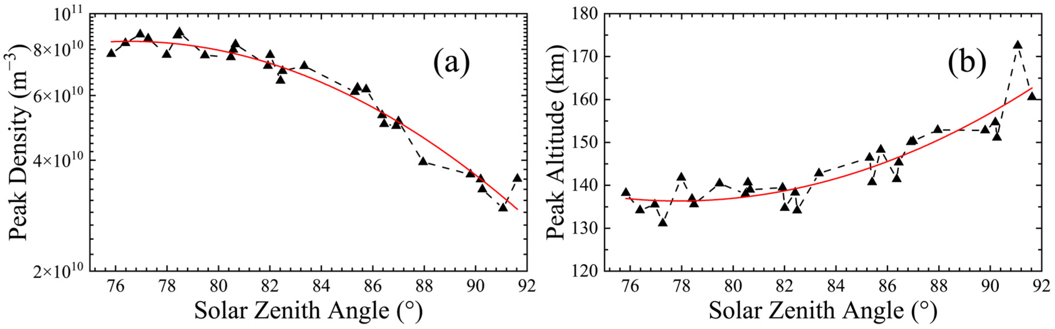
The variation of the solar zenith angle will closely affect the solar irradiance in the Martian ionosphere. For the M2 layer, the main effect of solar irradiance is photoionization by the EUV radiation. We statistically analyzed the electron peak density and peak height using MAVEN’s Radio Occultation Science Experiment (ROSE) data on March 2022 at different solar zenith angles, and the results are shown in Figure 2. It shows that the peak density decreases linearly as the zenith angle in Figure 2a. And in Figure 2b, the peak height increases linearly with the solar zenith angle. A possible explanation is that an increase in the solar zenith angle will lead to a decrease in solar irradiance and a weakening of photoionization, which affects the electron production rate and thus reduces the peak density. At the same time, an increase in the solar zenith angle also leads to a decrease in the refractive depth, so that soft X-rays and solar EUV radiation are unable to penetrate deeper into the ionosphere, resulting in the elevation of the peak height.
3.2. The Correlation between Martian Ionosphere and Solar Flares
When a solar flare occurs, the Sun will burst a large amount of energy with various radiation and energetic charged particles [23]. Based on the soft X-ray intensity in the wavelength range of 1 to 8 Å, flares can be divided into A, B, C, M and X categories [24]. X-class flares are intense ones, M-class are moderate flares, and C-class and below are minor ones [25]. Using the data obtained from the continuous observation of solar activity by the Solar and Heliospheric Observatory (SOHO) satellite, we found C-class flares on 26 August 2016, 29 November 2020, and 26 August 2021. The profiles of these three days are fitted to obtain the model parameters, as shown in Table 2. These three cases are compared with the day without flares. The comparison days are selected according to the date, the proximity of the local time, the similarity of the solar zenith angle, and the complete data. The corresponding dates are 9 August 2016, 1 December 2020, and 29 August 2021, respectively. The results show that the peak density of M1 increases by 33.4%, 13.2% and 7.4%, respectively. The peak height of the M1 layer decreases by 0.1%, 10.2% and 4.4%. The ratio of the M1 layer peak height to M2 layer peak height decreased by 1.5%, 7%, and 3.5%, while the ratio of the M1 layer peak density to M2 layer peak density increased by 7.6%, 3.6%, and 3.2%, respectively.
The comparison between the profiles with and without flares is shown in Figure 3a,c,e, where the red circles are the ionospheric profiles when the flare occurs, fitted with red dashed lines, and the blue circles are the profiles in the absence of the flare, fitted with blue dashed lines. It can be found that during the flares, the electron density above 200 km increases significantly, indicating the occurrence of the flare may promote photoionization on the upper ionosphere. But the peak density and height of the M2 layer are basically unchanged. The variation in the M1 layer is shown in Figure 3b,d,f where the electron density in the M1 layer below 110 km increases with decreasing altitude. Meanwhile, the peak density of the M1 layer increases and the peak altitude decreases.
It can be seen that both simulation and observation show that flares mainly affect the electron density in the M2 layer above 200 km and in the M1 layer. A possible explanation is that the source of ionization in the M2 layer is the solar EUV [5], while a large amount of energy will be released when the flare occurs, especially in the visible light, X-ray and EUV [26]. Absorption by the Martian ionosphere will result in an enhancement of the ionospheric electron density. Therefore, the three flares are followed by an increase in electron density above 200 km in Figure 3. On the other hand, the enhancement of solar activity will make the short-wavelength radiation more enhanced [27,28]. The source of ionization in the M1 layer is soft X-rays, which can penetrate into the lower Martian atmosphere [19] and ionize to produce more ion-electron pairs in the lower ionosphere [29]. Therefore, the electron density in the M1 layer in Figure 3 increases.
3.3. The Effect of Martian Dust Storm on the Ionospheric Profile
Mars is a desert planet with dust storms of different scales on its surface [3]. Sand particles in dust storms can affect the density, temperature, wind field and surface pressure in the atmosphere by absorbing the heat from solar shortwave radiation, thus affecting the Martian ionosphere [30,31,32]. The sand amount in the Martian atmosphere varies seasonally [3]. The northern hemisphere is located near the perihelion in autumn and winter with insolation enhancement, which will have a greater impact on atmospheric fluctuations [3]. As a result, the atmospheric sand content is higher in fall and winter, which is known as the dust storm season [3].
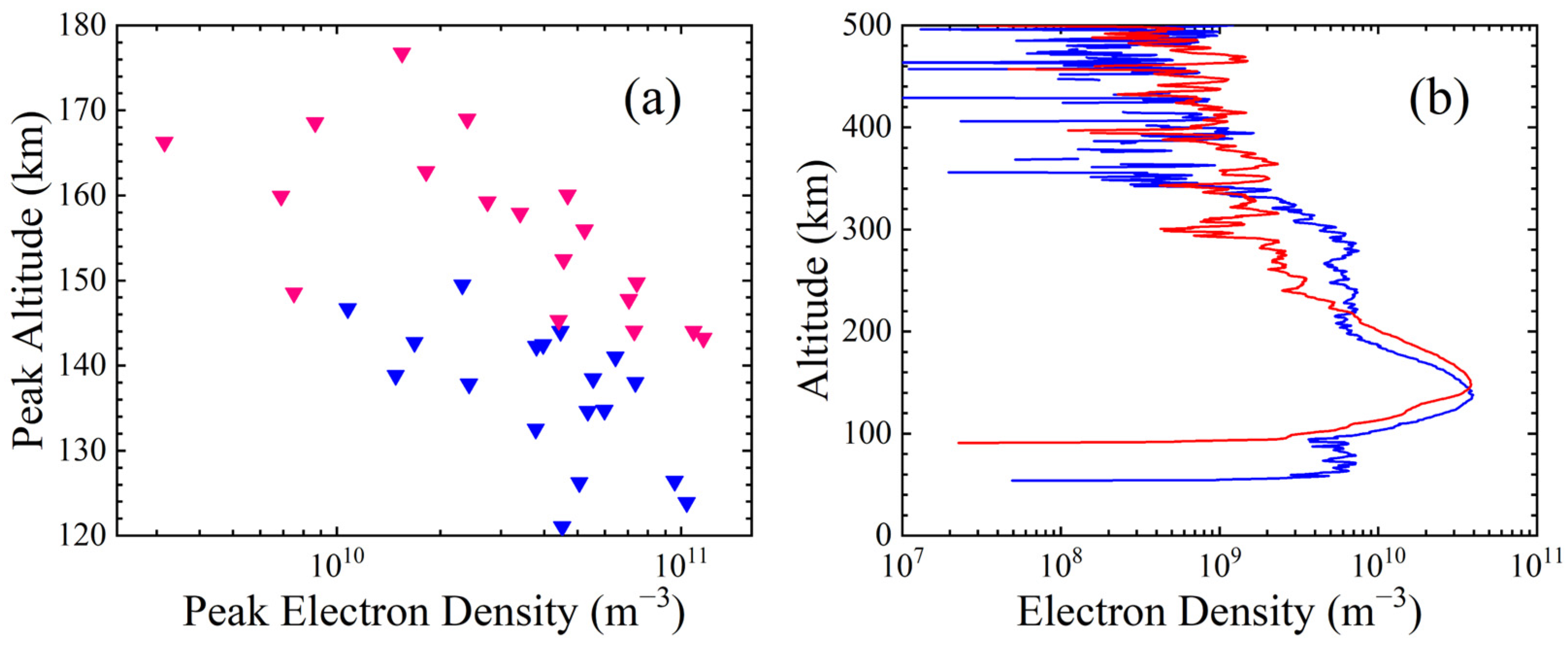
To investigate the effect of dust storms on the ionosphere, we have counted the peak heights and corresponding peak densities of the ionospheric electrons by MAVEN ROSE for 36 months from 2016 to 2022. The red triangles in Figure 4a exhibit 18 months in the fall and winter seasons, and the other 18 months colored in blue are revealed for spring and summer. It shows that the peak height of electrons in spring and summer is between 120–145 km, with an average height of 136.7 km and a peak density of 4.73 × . In autumn and winter, the peak height is located between 147 and 170 km, the average height is 156.2 km, and the average peak density is 4.31 ×. All the observed data are fitted in Figure 4b, indicating the difference in electron density profile between dust storm season and non-dust storm season. During the dust storm, the overall height of the ionosphere increased by 19.5 km, and the peak density decreased by 4.2 ×. Therefore, dust storms will elevate the peak height of ionospheric electrons and reduce the peak density. A possible explanation is the presence of dust storms may reduce the intensity of the solar EUV, which in turn reduces the peak density of the ionosphere. In addition, the elevation of the ionosphere will transport neutral molecules (e.g., H2O) and ions upwards [9]. The enhanced upward transport of H2O will accelerate the escape of H atoms [9], thus affecting the evolution of the Martian atmosphere, which is consistent with the research of Stone et al. (2020) [9].
4. Conclusions
In this paper, the Martian ionosphere is fitted through the NGIMS in situ observation and ROSE occultation observation collected in MAVEN’s KP data set. A one-dimensional profile model is established for the Martian ionospheric , , , , , and electron. The peak height and peak density at different solar zenith angles in March 2022 are calculated. The ionospheric electron density profiles when flares occurred on 26 August 2016, 29 November 2020 and 26 August 2021 are analyzed, and the corresponding models are compared. The peak height and peak density of the electron profile during the Martian dust storm season and the non-dust storm season from 2016 to 2022 are counted and tabulated. Based on the MAVEN data and the model established by the Chapman equation, the following distribution characteristics of the Martian ionosphere are obtained:
- (1)
- The main peak of the Martian ionospheric M2 layer is 140 km, and the M1 layer peak is 110 km. The peak density of the dayside ionosphere decreases with the increase of the solar zenith angle, and the peak height increases with the increase of the solar zenith angle.
- (2)
- When the three flares occur, the electron density in the M2 layer above 200 km increases. The peak density of the M1 layer increased by 33.4%, 13.2% and 7.4%, and the peak height of the M1 layer decreased by 0.1%, 10.2% and 4.4%, respectively.
- (3)
- The Martian ionosphere is affected by global dust storms. The peak height of the ionosphere in the dust storm season is 19.5 km higher than that in the non-dust storm season, and the peak density decreases by 8.9%.
Author Contributions
Conceptualization, S.Q.; methodology, S.Q. and R.L.; investigation, R.L.; writing—original draft preparation, S.Q.; writing—review and editing, W.S.; visualization, R.L.; supervision, S.Q.; project administration, S.Q.; funding acquisition, S.Q. All authors have read and agreed to the published version of the manuscript.
Funding
This research was funded by the Fundamental Research Funds for the Central Universities, CHD (NO. 300102263205), the consulting project by the Institute of Earth Environment (NO. 220126230684), and the West Light Cross-Disciplinary Innovation team of the Chinese Academy of Sciences (NO. E1294301).
Data Availability Statement
The data access to MAVEN is https://pds-ppi.igpp.ucla.edu/mission/MAVEN/MAVEN/LPW (accessed on 22 April 2024).
Acknowledgments
We thank the Fundamental Research Funds for the Central Universities, CHD, and the West Light Cross-Disciplinary Innovation team of the Chinese Academy of Sciences. We acknowledge the data usage of NASA’s MAVEN mission. The authors would like to thank Mingli Zour from China University of Geosciences for her suggestion on the data process.
Conflicts of Interest
The authors declare no conflicts of interest.
References
- Fallows, K.; Withers, P.; Gonzalez, G. Response of the Mars Ionosphere to Solar Flares: Analysis of Mgs Radio Occultation Data. J. Geophys. Res. Space Phys. 2015, 120, 9805–9825. [Google Scholar] [CrossRef]
- Cao, Y.T.; Niu, D.D.; Cui, J.; Wu, X.S. Reviews of Venusian and Martian Ionospheres. Rev. Geophys. Planet. Phys. 2021, 52, 528–542. [Google Scholar]
- Wu, Z.P.; Li, J.; Li, T.; Cui, J. The Dust Storm and Its Interaction with Atmospheric Waves on Mars. Rev. Geophys. Planet. Phys. 2021, 52, 402–415. [Google Scholar]
- Rishbeth, H.; Mendillo, M. Ionospheric Layers of Mars and Earth. Planet. Space Sci. 2004, 52, 849–852. [Google Scholar] [CrossRef]
- Hanson, W.; Sanatani, S.; Zuccaro, D. The Martian Ionosphere as Observed by the Viking Retarding Potential Analyzers. J. Geophys. Res. 1977, 82, 4351–4363. [Google Scholar] [CrossRef]
- Chen, R.; Cravens, T.; Nagy, A. The Martian Ionosphere in Light of the Viking Observations. J. Geophys. Res. Space Phys. 1978, 83, 3871–3876. [Google Scholar] [CrossRef]
- Liu, L.; Wan, W.; Chen, Y.; Le, H. Solar Activity Effects of the Ionosphere: A Brief Review. Chin. Sci. Bull. 2011, 56, 1202–1211. [Google Scholar] [CrossRef]
- Mendillo, M.; Withers, P.; Hinson, D.; Rishbeth, H.; Reinisch, B. Effects of Solar Flares on the Ionosphere of Mars. Science 2006, 311, 1135–1138. [Google Scholar] [CrossRef]
- Stone, S.W.; Yelle, R.V.; Benna, M.; Lo, D.Y.; Elrod, M.K.; Mahaffy, P.R. Hydrogen Escape from Mars Is Driven by Seasonal and Dust Storm Transport of Water. Science 2020, 370, 824–831. [Google Scholar] [CrossRef]
- Withers, P.; Felici, M.; Mendillo, M.; Moore, L.; Narvaez, C.; Vogt, M.F.; Oudrhiri, K.; Kahan, D.; Jakosky, B.M. The Maven Radio Occultation Science Experiment (Rose). Space Sci. Rev. 2020, 216, 61. [Google Scholar] [CrossRef]
- Dong, C.; Bougher, S.W.; Ma, Y.; Toth, G.; Lee, Y.; Nagy, A.F.; Tenishev, V.; Pawlowski, D.J.; Combi, M.R.; Najib, D. Solar Wind Interaction with the Martian Upper Atmosphere: Crustal Field Orientation, Solar Cycle, and Seasonal Variations. J. Geophys. Res. Space Phys. 2015, 120, 7857–7872. [Google Scholar] [CrossRef]
- Erdal, Y.; Knížová, P.K.; Georgieva, K.; Ward, W. A Review of Vertical Coupling in the Atmosphere–Ionosphere System: Effects of Waves, Sudden Stratospheric Warmings, Space Weather, and of Solar Activity. J. Atmos. Sol. Terr. Phys. 2016, 141, 1–12. [Google Scholar]
- Krebs, G.D. Maven (Mars Scout 2). Available online: https://space.skyrocket.de/doc_sdat/maven.htm (accessed on 24 January 2024).
- Steckiewicz, M.; Mazelle, C.; Garnier, P.; André, N.; Penou, E.; Beth, A.; Sauvaud, J.A.; Toublanc, D.; Mitchell, D.L.; McFadden, J.P.; et al. Altitude Dependence of Nightside Martian Suprathermal Electron Depletions as Revealed by Maven Observations. Geophys. Res. Lett. 2015, 42, 8877–8884. [Google Scholar] [CrossRef]
- Jakosky, B.M.; Lin, R.P.; Grebowsky, J.M.; Luhmann, J.G.; Mitchell, D.F.; Beutelschies, G.; Priser, T.; Acuna, M.; Andersson, L.; Baird, D.; et al. The Mars Atmosphere and Volatile Evolution (Maven) Mission. Space Sci. Rev. 2015, 195, 3–48. [Google Scholar] [CrossRef]
- Fox, J.L.; Galand, M.I.; Johnson, R.E. Energy Deposition in Planetary Atmospheres by Charged Particles and Solar Photons. Space Sci. Rev. 2008, 139, 3–62. [Google Scholar] [CrossRef]
- Chapman, S. The Absorption and Dissociative or Ionizing Effect of Monochromatic Radiation in an Atmosphere on a Rotating Earth. Proc. Phys. Soc. 1931, 43, 26. [Google Scholar] [CrossRef]
- Chapman, S. The Absorption and Dissociative or Ionizing Effect of Monochromatic Radiation in an Atmosphere on a Rotating Earth Part II. Grazing Incidence. Proc. Phys. Soc. 1931, 43, 483. [Google Scholar] [CrossRef]
- Zhang, T.; Liu, L.; Chen, Y.; Le, H.; Zhang, R.; Zhang, H. Response of Martian Ionospheric Electron Density to Changes in Solar Radiation. Chin. J. Geophys. 2022, 65, 1571–1580. [Google Scholar]
- Fallows, K.; Withers, P.; Matta, M. An Observational Study of the Influence of Solar Zenith Angle on Properties of the M1 Layer of the Mars Ionosphere. J. Geophys. Res. Space Phys. 2015, 120, 1299–1310. [Google Scholar] [CrossRef]
- Hantsch, M.H.; Bauer, S.J. Solar Control of the Mars Ionosphere. Planet. Space Sci. 1990, 38, 539–542. [Google Scholar] [CrossRef]
- Sánchez-Cano, B.; Radicella, S.M.; Herraiz, M.; Witasse, O.; Rodríguez-Caderot, G. Nemars: An Empirical Model of the Martian Dayside Ionosphere Based on Mars Express Marsis Data. Icarus 2013, 225, 236–247. [Google Scholar] [CrossRef]
- Harvey, K.L. The Explosive Phase of Solar Flares. Sol. Phys. 1971, 16, 423–430. [Google Scholar] [CrossRef]
- Veronig, A.; Temmer, M.; Hanslmeier, A.; Otruba, W.; Messerotti, M. Temporal Aspects and Frequency Distributions of Solar Soft X-Ray Flares. Astron. Astrophys. 2002, 382, 1070–1080. [Google Scholar] [CrossRef]
- Winter, L.M.; Balasubramaniam, K. Using the Maximum X-Ray Flux Ratio and X-Ray Background to Predict Solar Flare Class. Space Weather 2015, 13, 286–297. [Google Scholar] [CrossRef]
- Tsurutani, B.T.; Judge, D.L.; Guarnieri, F.L.; Gangopadhyay, P.; Jones, A.R.; Nuttall, J.; Zambon, G.A.; Didkovsky, L.; Mannucci, A.J.; Iijima, B.; et al. The October 28, 2003 Extreme Euv Solar Flare and Resultant Extreme Ionospheric Effects: Comparison to Other Halloween Events and the Bastille Day Event. Geophys. Res. Lett. 2005, 32, L03S09. [Google Scholar] [CrossRef]
- Woods, T.N.; Eparvier, F.G. Solar Ultraviolet Variability During the Timed Mission. Adv. Space Res. 2006, 37, 219–224. [Google Scholar] [CrossRef]
- Lean, J.L.; Woods, T.N.; Eparvier, F.G.; Meier, R.R.; Strickland, D.J.; Correira, J.T.; Evans, J.S. Solar Extreme Ultraviolet Irradiance: Present, Past, and Future. J. Geophys. Res. Space Phys. 2011, 116, A01102. [Google Scholar] [CrossRef]
- Schunk, R.; Nagy, A. Ionospheres: Physics, Plasma Physics, and Chemistry; Cambridge University Press: Cambridge, UK, 2009. [Google Scholar]
- Gierasch, P.J.; Goody, R.M. The Effect of Dust on the Temperature of the Martian Atmosphere. J. Atmos. Sci. 1972, 29, 400–402. [Google Scholar] [CrossRef]
- Zhou, Y.H.; Salstein, D.A.; Xu, X.Q.; Liao, X.H. Global Dust Storm Signal in the Meteorological Excitation of Mars’ Rotation. J. Geophys. Res. Planets 2013, 118, 952–962. [Google Scholar] [CrossRef]
- Forget, F.; Montabone, L. Atmospheric Dust on Mars: A Review. In Proceedings of the 47th International Conference on Environmental Systems, Charleston, SC, USA, 16–20 July 2017; p. 175. [Google Scholar]
Figure 1.
Fitted profiles for various ions (a–g) and the electron (h). The electron data on March 2022 are derived from MAVEN’s Radio Occultation Science Experiment, ROSE, and the ion data on 1 January 2022 are obtained from KP.
Figure 1.
Fitted profiles for various ions (a–g) and the electron (h). The electron data on March 2022 are derived from MAVEN’s Radio Occultation Science Experiment, ROSE, and the ion data on 1 January 2022 are obtained from KP.

Figure 2.
The distribution of the ionospheric peak density (a) and the peak height (b) with the zenith angle, where the black triangle is the measured peak density, and the red curve is the linear fitted profile. The data on March 2022 are derived from ROSE.
Figure 2.
The distribution of the ionospheric peak density (a) and the peak height (b) with the zenith angle, where the black triangle is the measured peak density, and the red curve is the linear fitted profile. The data on March 2022 are derived from ROSE.

Figure 3.
Comparison of electronic observations and fitted curves at the time of the flare and in the absence of the flare. (a,c,e): the red circle represents the observation data when the flare occurs, and the red dotted line is its fitting line. The blue circle represents the observation data when the flare does not occur, and the blue dotted line is its fitting line. (b,d,f) are the comparison of the M1 layer changes. The red line indicates that the flare occurred, and the blue line indicates that the flare did not occur. The data on 26 August 2016 for Figures (a,b) are derived from MAVEN’s ROSE experiment. The data for Figures (c,d) are from ROSE on 29 November 2020; the data for Figures (e,f) are on 26 August 2021.

Figure 4.
(a) Distribution of peak density with peak height during dust storm periods (i.e., fall and winter, red triangles) and non-dust storm periods (i.e., spring and summer, blue ones). (b) The 18-month average electron profile of the dust storm period (red curve) and the non-dust storm period (blue curve). The data are based on MAVEN’s ROSE experiment from 2016 to 2022.


Table 1.
Fitting results of the particles.
| Kind of the Particle | a | |||
|---|---|---|---|---|
| O | 260.001 | 274.924 | 106.937 | 3.0463 |
| 3721.223 | 187.554 | 1.578 | 0.019 | |
| 3933.944 | 198.555 | 6.906 | 0.076 | |
| 1218.344 | 187.160 | 3.253 | 0.013 | |
| 315.442 | 205.165 | 16.069 | 0.241 | |
| 177.109 | 213.210 | 27.311 | 0.470 | |
| 1589.037 | 239.902 | 39.292 | 0.457 |
Table 2.
The solar flare effects on model parameters.
| Date | (m−3) | (m−3) | (km) | (km) | ||
|---|---|---|---|---|---|---|
| 26 August 2016 | 1.296 × 10¹¹ | 5.23 × 10¹⁰ | 147.7 | 117.6 | 0.378 | 0.796 |
| 9 August 2016 | 1.382 × 10¹¹ | 3.92 × 10¹⁰ | 145.1 | 117.7 | 0.302 | 0.811 |
| 29 November 2020 | 9.988 × 10¹⁰ | 4.56 × 10¹⁰ | 141.2 | 109.7 | 0.457 | 0.777 |
| 1 December 2020 | 9.569 × 10¹⁰ | 4.028 × 10¹⁰ | 144.1 | 122.1 | 0.421 | 0.847 |
| 26 August 2021 | 5.82 × 10¹⁰ | 2.727 × 10¹⁰ | 149.7 | 114.7 | 0.469 | 0.766 |
| 29 August 2021 | 5.79 × 10¹⁰ | 2.54 × 10¹⁰ | 146.8 | 117.6 | 0.437 | 0.801 |
Disclaimer/Publisher’s Note: The statements, opinions and data contained in all publications are solely those of the individual author(s) and contributor(s) and not of MDPI and/or the editor(s). MDPI and/or the editor(s) disclaim responsibility for any injury to people or property resulting from any ideas, methods, instructions or products referred to in the content. |
© 2024 by the authors. Licensee MDPI, Basel, Switzerland. This article is an open access article distributed under the terms and conditions of the Creative Commons Attribution (CC BY) license (https://creativecommons.org/licenses/by/4.0/).
Share and Cite
MDPI and ACS Style
Qiu, S.; Li, R.; Soon, W. An Investigation on the Distribution of Martian Ionospheric Particles, Based on the Mars Atmosphere and Volatile Evolution (MAVEN). Universe 2024, 10, 196. https://0-doi-org.brum.beds.ac.uk/10.3390/universe10050196
AMA Style
Qiu S, Li R, Soon W. An Investigation on the Distribution of Martian Ionospheric Particles, Based on the Mars Atmosphere and Volatile Evolution (MAVEN). Universe. 2024; 10(5):196. https://0-doi-org.brum.beds.ac.uk/10.3390/universe10050196
Chicago/Turabian StyleQiu, Shican, Ruichao Li, and Willie Soon. 2024. "An Investigation on the Distribution of Martian Ionospheric Particles, Based on the Mars Atmosphere and Volatile Evolution (MAVEN)" Universe 10, no. 5: 196. https://0-doi-org.brum.beds.ac.uk/10.3390/universe10050196
Note that from the first issue of 2016, this journal uses article numbers instead of page numbers. See further details here.