Article

Changes in and Recovery of the Turbulence Properties in the Magnetosheath for Different Solar Wind Streams

by
Liudmila Rakhmanova
*,
Alexander Khokhlachev
,
Maria Riazantseva
,
Yuri Yermolaev
and
Georgy Zastenker
Space Research Institute, Russian Academy of Sciences, 117997 Moscow, Russia
*
Author to whom correspondence should be addressed.
Submission received: 14 February 2024 / Revised: 11 April 2024 / Accepted: 23 April 2024 / Published: 26 April 2024
(This article belongs to the Section Space Science)

Abstract

:
Solar wind is known to have different properties depending on its origin at the Sun. In addition to the differences in plasma and magnetic field parameters, these streams differ due to the properties of turbulent fluctuations involved in the flow. The present study addresses the changes in the turbulence properties in the magnetosheath—the transition region in front of the magnetosphere. This study is based on statistics from the simultaneous measurements of magnetic field fluctuations in the solar wind and in the magnetosheath. Both the dayside and flank magnetosheath regions are focused on to detect the evolution of the turbulent fluctuations during their flow around the magnetosphere. Turbulent cascade is shown to save its properties for fast solar wind streams. Conditions favorable for the preservation of the turbulence properties at the bow shock may correspond to the increased geoefficiency of large-scale solar wind structures.

1. Introduction

Solar wind (SW) originating at different solar sources has different effects on the magnetosphere. Various large-scale interplanetary phenomena may be distinguished by different kinetic and magnetic energy, deviations in the interplanetary magnetic field (IMF) vector from the ecliptic plane, and the SW speed. While the increased geoefficiency of the disturbed SW streams (interplanetary coronal mass ejections (ICMEs) including compressed regions (Sheath) ahead, corotating interaction regions (CIRs)) are generally known [1,2,3,4,5,6], the most significant factors and direct processes that underlie the difference in the magnetosphere response are still debated.
Exploration of the SW effects on the magnetosphere is usually prepared with the help of statistics from the SW measurements [5,6,7,8]. However, there is a magnetosheath (MSH) in front of the magnetopause that modifies the SW and IMF parameters substantially. Plasma becomes heated, decelerated, and compressed at the bow shock (BS)—the outer boundary of the MSH. Plasma and magnetic field downstream of the BS exhibit a high level of fluctuations in a wide range of scales, including ion and sub-ion scales. A zoo of instabilities, ion- and sub-ion-scale structures are the main sources of the MSH fluctuations, and consequently these fluctuations cannot be reproduced by MHD descriptions of the flow around the magnetosphere [9,10]. Also, high-speed jets may be found in the MSH, which can directly hit the magnetopause [11,12]. Small-scale plasma structures may be modified in the MSH [13] and the parameters in front of the magnetopause (including important magnetospheric drivers) may differ substantially from those observed in the L1 [14]. The sign of the Bz IMF component may be changed in the MSH [15,16], including periods of large-scale SW disturbances [17]. Periods of low Mach number SW flows (attributed typically to the ICMEs) result in additional kinetic-scale effects in the boundary layers of the magnetopause [4]. Thus, neglecting the MSH processes may result in the reduced predictability of the SW effect on the magnetosphere.
In the SW and in the MSH, variations in the parameters may be analyzed in a framework of turbulence. Turbulent fluctuations form the cascade that spans over a wide range of scales. This cascade is typically observed as a spectrum of the fluctuations that can be described by power laws with power exponents (slopes) varying in different ranges of scales (see [18,19,20] for theory and detailed reviews of the study of turbulent fluctuations in the near-Earth plasma). The properties of turbulent fluctuations can be analyzed as a proxy for the leading processes at different scales. Typically, in the undisturbed SW, the frequency spectrum of turbulent fluctuations follows the f−1 power law at the scales above ~106 km, then breaks and follows the f−5/3 law up to the ion scales (inertial range or MHD scales). At the ion scales (around proton gyroradius or proton inertial length), the spectrum breaks and transition to ion kinetic scales occurs. At smaller scales, the energy dissipation and heating of particles is supposed to take place. The spectrum at the kinetic scales typically follows the f−α power law with α varying from −4 to −2.
A large network of spacecraft measurements in the SW and MSH show changes in the turbulence properties at the BS and in the dayside MSH. Generally, at the MHD scales, the f−5/3 scaling of the magnetic field and ion flux/density fluctuations ruins at the BS and tends to restore closer to the magnetopause and at the flanks [21,22,23,24]. Statistical studies in the MSH reveal that at the kinetic scales, spectra generally do not deviate from those that occurred in the SW [21,23]. However, the direct comparison of spectra upstream and downstream of the BS demonstrates the steepening of spectra at the BS, particularly during the disturbed SW periods [24]. Moreover, sometimes, f−5/3 scaling in the inertial range may be found downstream of the BS [25]. Turbulence properties differ behind the quasi-perpendicular and quasi-parallel BS as well [26,27,28,29,30]. Thus, the picture of the modification of turbulence properties during plasma propagation from the SW to the magnetopause is still unclear.
The most dramatic changes in the turbulence properties behind the BS are observed for the disturbed SW flows associated with ICMEs and CIRs [24]. Moreover, there are differences in the way of turbulence development when plasma moves away from the BS. The different effect on the magnetosphere by various SW streams together with the suggestion of different ways of turbulence development in the MSH for these streams underlines the contribution of the MSH turbulence to the SW–magnetosphere coupling. Thus, the way of turbulence development in the MSH should be clarified for different types of SW. The present study focuses on this topic and presents the first statistical results. This study is based on the comparison of the simultaneous observation of the turbulence properties on two spacecraft—in the SW in an orbit around Lagrangian L1 point (Wind) and in different regions inside the MSH (THEMIS), including the dayside and flank MSH. Cases of quasi-perpendicular BS are considered to avoid the additional effects of the BS properties and mixing of the results. The methods of data selection and processing are described in Section 2, the statistical results are presented in Section 3, discussed in Section 4, and summarized in Section 5.

2. Materials and Methods

2.1. Magnetosheath Crossings Selection

THEMIS [31] measurements in the MSH are considered during the years 2008 and 2014. The periods correspond to solar minimum and maximum that guarantees the variability of the background SW conditions. THEMIS mission includes 5 spacecraft with orbits organized differently during the considered periods. Data of all 5 spacecraft were analyzed manually to detect the MSH crossings. The selection criteria for the crossing were used as follows: (1) the interval duration was larger than 1.5 h and (2) fast magnetic field measurements were available. If spacecraft were located close to each other (1 RE or less), data from one of the spacecraft were chosen based on data quality. Altogether, we managed to collect 274 crossings with a duration ranging from 1.5 to 11 h and total duration of 800 h. We used ESA plasma measurements [32] with 3–4 s sampling and FGM data [33] with 0.25 s sampling. Data were downloaded from https://cdaweb.gsfc.nasa.gov/ (accessed on 1 December 2023) database.
To analyze the dynamics of the turbulence properties, the MSH crossings were cut into intervals of 68 min duration with 34 min sliding window. The duration of intervals must provide a large enough number of data points for the calculation of a fluctuation spectrum and stability of background conditions. Time intervals of 68 min duration were chosen to meet these conditions. The intervals’ overlap guarantees that all the structures during the MSH crossing would be included in the statistical analysis. Altogether, 1087 intervals were collected.
Each of the analyzed intervals was attributed to the SW type according to the catalog [34] (available online http://iki.rssi.ru/pub/omni/catalog/ (accessed on 1 December 2023)). The catalog is based on the OMNI database, which refers to the SW data shifted to the BS nose; hence, no time shift is required in this case. Figure 1 presents the location of THEMIS spacecraft during each interval, colored according to the SW type. The statistics include the following: slow undisturbed SW (“Slow”)—41% of cases, corotating interaction regions ahead of high-speed streams from coronal holes (“CIR”)—15% of cases, ICME—16% of cases, fast SW (“Fast”)—14% of cases, and regions associated with the heliospheric current sheet (“HCS”)—7%. For 7% of cases, the SW type cannot be attributed to the interval, as the start time of a large-scale phenomenon lies in the middle of the interval. Compressed regions ahead of the ICMEs (“Sheath”) are not covered by the statistics. Also, the ICME statistics include both ICMEs with and without Sheath regions ahead.
As shown in Figure 1, the statistics can be divided into two parts—the dayside MSH (XGSE > −10 RE) and the flank MSH (XGSE = <−10 RE). Note, this classification is arbitrary and not commonly used as typically turbulence is not considered in the tailward regions. In the analyzed statistics, 35% of cases refer to the flank MSH and the other 65% of cases refer to the dayside MSH. Except for the HCS, all the considered SW types are represented both in the dayside and flank MSH.
To check the configuration of the BS for each interval, the θBN angle was calculated. The calculation procedure is described in detail in the paper by Shevyrev and Zastenker [35]. The MSH spacecraft position was traced upstream to the BS along the flow lines determined by the gasdynamic model [36]. Then, time-shifted Wind data were used to calculate an angle between the IMF and a local normal to the BS in this point. Intervals with θBN < 45° were eliminated from the statistics. Note, such a method of separation between quasi-parallel and quasi-perpendicular BS has inaccuracies that come from (1) the use of modeled positions of the BS together with MHD/HD models of flow lines behind the BS and (2) errors in the calculation of a time lag from the SW spacecraft to the BS. However, alternative methods based on in situ properties [37,38] require large statistics to provide the correct thresholds for separation for various SW conditions and various positions inside the MSH. For the purposes of the present study, the determination of a time lag of plasma propagation from Wind to the BS with ~10 min accuracy (see [39] for detailed comparison of the common methods) is enough as the turbulence properties are considered on ~1 h intervals. Also, the effects of the quasi-parallel BS can sometimes be found for 45° < θBN < 60° [37]. The present study does not account for these effects and uses the common formal criteria of θBN > 45° to determine the quasi-perpendicular BS cases.

2.2. Calculating a Time Lag between the Solar Wind and Magnetosheath Dataset

For each MSH crossing by the THEMIS spacecraft, the corresponding time period of the SW measurements was analyzed. Measurements for the SW were performed by the Wind spacecraft. SWE instrument [40] plasma measurements were used with 92 s time resolution and MFI [41] magnetic field measurements were used with 0.092 s time resolution.
To determine the plasma propagation time between the spacecraft, the Wind time series were shifted by T0 = dXGSE/<V>, where dXGSE is the difference in the XGSE coordinates of the Wind and THEMIS spacecraft and <V> was the mean SW speed during the MSH crossing. T0 gave the first approximation of the shift, which did not account for the plasma deceleration in the MSH and for differences in the structure speeds. Then, correlation analysis was adopted to specify the propagation time. The THEMIS density time profile was interpolated to have a similar sampling with the Wind density time profile. Correlation coefficient R was calculated between the SW and the MSH time series of density measurements for shifts T varied from T0 − 40 min to T0 + 40 min. Time shift T1, which corresponded to the maximum of the correlation function R(T), was chosen as the required propagation time. All the propagation times were visually inspected. Correlation analysis provided a good matching of the plasma structures on the two spacecraft for 50% of cases. The other cases referred to either the absence of the plasma structures for matching or recurring structures, which made the time lag determination controversial. For such cases, the time lag was corrected manually to provide the best correspondence between time profiles on the two spacecraft. Typical errors in the time lag estimation (due to difference in speed of different structures) are ~10 min. As further spectral analysis operates with ~1 h time intervals, the errors of the time lags do not influence the results. The problems of the method are discussed in more detail in [24].
Figure 2 presents an example of the considered MSH crossing by the THEMIS-C spacecraft on 15 October 2008. THEMIS-C was located at {7; −14; −5} RE in the dayside MSH, Wind was located at {209; 93; −3} RE in the SW in an orbit around L1 point. Panel (Figure 2a) presents density measurements by THEMIS-C (black line) and by Wind (red line). Panels (Figure 2b) and (Figure 3c) show the magnetic field components and magnitude in the SW and MSH, respectively. The SW time series were shifted by 3660 s, which gave the maximum correlation between the SW and MSH density profiles R = 0.5. THEMIS-C was scanning the MSH and entered the magnetosphere at 17:00. High-resolution magnetometer data were absent before 14:30 (as shown in Figure 2c), and the interval 14:30–17:00 was chosen for the analysis (marked by the grey shadow in Figure 2). The interval exhibits good correspondence between the SW and MSH structures both for the plasma and magnetic field components despite the large separation along the YGSE axis—~107 RE. Note, the intervals that exhibited no visual correspondence were eliminated from the study.
After assuring observation of the same plasma by the two spacecraft, the interval of the crossing was cut into shorter 68 min intervals for spectral analysis. The duration of the time interval was chosen to include the number of data points that can be presented in a form N = 2M to fulfill the requirements of further Fourier analysis. The time resolutions of the magnetometers on board the Wind and THEMIS spacecraft were different, which resulted in a different duration of intervals for upstream and downstream regions. For Wind, the intervals had a 50 min duration and were chosen in such a way that the centers of the SW and MSH intervals matched. Black and red dashed vertical lines in Figure 2a–c show an example of the analyzed intervals for THEMIS-C and Wind, respectively.

2.3. Spectral Analysis

The present study adopts Fourier transform to obtain the properties of a spectrum of turbulent fluctuations. The calculated spectra were smoothed in the frequency space with the Hamming window. An example of the resulting spectra is presented in Figure 2d. The red line corresponds to the spectrum in the SW and the black line refers to the spectrum in the MSH. Vertical arrows denote plasma characteristic scales for each spacecraft, defined as FC = eB/mc (e, m are proton charge and mass, B is mean magnetic field, c is the speed of light), FL = V/2πL, L = c/ωp, ωp = (4πne2/m)1/2 (V is mean plasma bulk speed, L is proton inertial length, ωp is proton plasma frequency, n is mean proton density), FR = V/2πR, R = Vt/2πFc (R is proton thermal gyroradius, Vt is the most probable proton thermal speed). These scales are typically associated with the break frequency and are attributed to the processes that underlie energy dissipation. However, the position of the break is still debated [42,43,44,45] and is out of the scope of the present paper.
Each spectrum was approximated with the help of automatic routine in log(frequency)-log(power) space. Firstly, the linear approximation was performed at the frequency ranges 0.01–0.1 Hz and min(Fch)-Fmax/2. Here, Fch is one of the characteristic frequencies Fc, FL, and FR. Fmax is the maximum frequency of the spectrum, determined by the Nyquist frequency. Secondly, the edges of the frequency ranges were changed (both enlarged and narrowed (where possible) by 10 points), and approximation was performed for the modified ranges. Final approximation was chosen to correspond to the minimum of the approximation errors. Each final approximation was checked visually and recalculated in case of bad correspondence to the observed spectrum.
Note that the wide bump typically presents in a dayside MSH spectrum at the scales around the break (see the black spectrum in Figure 2d). For ~20% of spectra in the dayside MSH, this bump makes the approximation at the MHD scales impossible. Also, the Wind MFI instrument provides measurements with a high level of noises at frequencies exceeding 0.7 Hz, which results in the flattening of the kinetic-scale part of a spectrum [45]. Visual control of the approximation procedure allows us to avoid errors due to noise without making strong restrictions on the signal to noise ratio. This approach works well when the statistics are not too large for visual checking. In the present study, for 8% of the spectra obtained from Wind, the approximation cannot be performed at the kinetic scales.
As shown in Figure 2d, in the SW, the spectrum follows the f−1.8±0.1 power law at the MHD scales and f−2.50±0.05 power law at the kinetic scales. The values of the scaling exponents (slopes) correspond to those observed typically in the undisturbed SW [46,47,48] and described by the models [49,50]. In the dayside MSH, the spectrum power increases, and spectral slopes change. At the MHD scales, the spectrum is characterized by the −1.2 ± 0.1 spectral exponent, which deviates from the simultaneous SW observations and from the Kolmogorov −5/3 scaling predicted by the theories of the developed turbulence [51]. At the transition scales, the bump occurs at frequencies close to FR and Fc (see arrows in Figure 2d). At the kinetic scales, the spectrum is characterized by the slope −2.7 ± 0.1, i.e., the spectrum is somewhat steeper than the corresponding spectrum in the SW.
An example of the plasma tracking in the SW and at the MSH flank and the corresponding spectra is presented in Figure 3 (the format is similar to Figure 2). Wind was located at {237; 85; 8} RE, THEMIS-C was located at {−52; 32; −5} RE. Figure 3a–c demonstrate good correspondence between the spacecraft pair measurements both in the plasma and magnetic field time profiles despite the large separation. Figure 3d shows the comparison of the registered spectra. Both spectra exhibit a similar power of fluctuations and similar scaling both at the MHD and at the kinetic scales. Kolmogorov scaling occurs at the MHD scales in the SW as well as in the MSH.
Figure 3. Example of the case on 11 January 2014. The same format as in Figure 2: (a) ion density in the SW (red line) and in the MSH (black line); (b) IMF magnitude and components measured by Wind; (c) magnetic field components and magnitude measured by THEMIS-C in the MSH, the SW data are shifted in time by 3660 s; (d) magnetic field fluctuation spectra registered in the SW (red line) and in the MSH (black line).
Universe 10 00194 g003

2.4. On the Validity of the Taylor Hypothesis

Usually, the Taylor hypothesis is adopted to consider the temporal variations instead of the space variations [52]. The method assumes that while plasma moves by the spacecraft with speeds significantly higher than the wave phase speed or the spacecraft speed, one can consider the temporal variations to be the result of turbulent structures convected by the spacecraft. In the SW, Alfvén waves are dominant with speeds several times lower than the plasma speed. At the BS, the plasma decelerates significantly and the Alfvén speed becomes comparable to the plasma speed. According to the analysis by [53], the application of the Taylor hypothesis does not change the properties of a spectrum as long as V/Va > 0.3 (Va is the Alfvén speed). In the present study, this criterion was checked and intervals with V/Va < 0.3 (7%) were eliminated from the study.
Another problem in the application of the Taylor hypothesis is the presence of dispersive wave modes in plasma like whistlers. However, these waves are supposed to be rare [54] and are not taken into account in the present study.

3. Results

3.1. Statistics

Altogether, 1087 interval pairs were collected during the years 2008 and 2014. This amount was reduced to 996 after adopting the criteria V/Va > 0.3 and further reduced to 784 after eliminating quasi-parallel BS cases. Note, the difference in the number of quasi-perpendicular and quasi-parallel cases comes from the way of MSH crossing detection: the crossing of quasi-parallel BS is typically superimposed by large-amplitude fluctuations, which prevent the correct detection of the BS. Thus, these periods are likely to be ignored when the MSH crossing was chosen. As the study concentrates on the quasi-perpendicular cases, such a manual elimination of quasi-parallel cases does not affect the results. Among these intervals, 536 corresponded to the dayside MSH and 248 corresponded to the flank MSH. A further reduction in the intervals amount was caused by the approximation procedure (presence of bumps or noise, see Section 2.3).
All obtained spectra were sorted according to the observed region (SW, dayside, and flank MSH) and then according to the SW type. Figure 4 presents the mean values of the spectra slopes at the MHD (upper panel) and kinetic (lower panel) scales for five types of the SW in the three considered locations. Error bars represent the standard error of the mean values. Note that according to Figure 1, there are no HCS intervals at the MSH flanks. Figure 4 shows that in the SW, the spectra typically have a slope from −1.8 to −1.6, which is close to the −5/3 scaling. At the kinetic scales, there is a clear difference betweenthe properties of turbulence for large-scale SW events. The SW of types Slow, HCS, and ICME are characterized by the mean slope <P2> = −2.5, while for the Fast and CIR types, the spectra are substantially steeper and follow f−2.85 scaling.
In the dayside MSH, the spectra are flatter at the MHD scales for all SW types. The mean slope varies slightly for different SW types. ICME and HCS events are the most modified with a mean value of <P1> = −1.15. CIR events are accompanied by the least modified slope—−1.3. The difference between the CIR and ICME/HCS events is rather small; however, it exceeds the standard errors of the means. At the kinetic scales, the difference in spectral properties is more pronounced. HCS and Slow events are accompanied by −2.8 scaling. For the Fast SW and CIRs, the spectra are characterized by the mean slope <P2> = −3.05. The steepest spectra are observed for ICMEs with the mean slope <P2> = −3.15.
At the MSH flanks, the spectra at the MHD scales are closer to those observed in the SW. However, the −5/3 scaling can be found only for CIR events. Slow and ICME periods are characterized by the mean slope <P1> = −1.4, while for the Fast SW, the slope is slightly closer to the one observed in the SW—<P1> = −1.45. At the kinetic scales, four detected types of the SW have similar scaling f−2.5. HCS events are not covered by our statistics at the flanks.

3.2. Modification of Spectral Slopes

Figure 4 aims to demonstrate the typical properties of different SW periods and the reliability of the statistics. To consider the modification of the spectral slopes at the BS and throughout the MSH, we defined the change inthe slope at the BS as ΔPa = (PaMSH − PaSW)/PaSW, where a = 1,2 for the MHD and kinetic scales, respectively. This value was considered for the dayside MSH as well as for the flank regions for different SW types. ΔP > 0 (ΔP < 0) refers to the steepening (flattening) of the spectrum in the MSH. Figure 5 presents the distributions for the MHD scales for the dayside MSH (Figure 5a, b) and for the flanks (Figure 5c,d). The statistics were divided into two groups for comparison—Slow, ICME, and CIR (panels Figure 5a,c) and Slow, HCS, and Fast (panels Figure 5b,d). Figure 6 presents in a similar way the statistics of the kinetic-scale slope changes. The mean and median values and standard deviations for each range of scales for both locations are summarized in Table 1. All the distributions demonstrate a wide spread of the changes in the scaling exponents, which resulted in large values of standard deviations. However, some features may be revealed. The errors of the mean values are low (<1%, not included in the Table 1).
It should be noted that considering the distributions of the spectral indices in each region (Figure 4), some cases do not correspond directly to the distributions of the changes in the slopes (Table 1). This effect is the most noticeable for ICME and CIR events. This is likely to be a result of insufficient statistics. The number of intervals in each distribution vary from 16 to 123, with the poorest statistics being collected for the MHD scales of ICME events. To check the influence of the distribution shape on the results, the median value was calculated for each distribution. The bolded values in Table 1 refer to the distributions for which a difference occurs between the mean and median values. The median values for these cases are presented in Figure 5 and Figure 6. We suggest that the distributions of the change in the spectral slopes have a more physical meaning for the results.
For all types of the SW, a significant flattening of the spectra at the MHD scales occurs at the BS, with the slope value changing by ΔP1 = 0.2–0.4. This change corresponds to the deviation from the original SW scaling by 20–40%.
Distributions in Figure 5c,d are shifted to the mean values of ΔP1 = 0 compared to those in Figure 5a,b. Hence, at the flanks, the spectra tend to restore the shape observed in the SW. However, during the Slow SW, the spectra stay significantly changed (ΔP1 = 0.17). Periods of Fast SW and CIR exhibit the most restored shape at the flank atthe MHD scales—<ΔP1> varies from −0.07 to −0.1. Statistics for the ICME events are small and do not demonstrate any particular distribution. However, the mean value of the slope change is similar to the one for the Slow SW, while the median value denotes somewhat flattened spectra.
The kinetic-scale part of the spectra demonstrates more variability. Figure 6 shows that at the BS, substantial steepening of the spectra occurs for the SW of types Slow and ICME. The mean change in the slope ΔP2 varies from 0.26 to 0.3. Periods of HCS are accompanied by less pronounced steepening ΔP2 = 0.16. During the CIRs and Fast SW streams, the spectral slopes are nearly unchanged at the BS.
At the flanks, the statistics for ICME events are quite limited. Slow SW and Fast SW demonstrate mean spectral slopes similar to those observed in the SW. However, the median value of the slope ΔP2median = −0.06 implies a slight flattening compared to the SW spectra. Fast SW exhibits the spectrum that matches the one in the SW. ICME events exhibit slightly steeper spectra than in the SW with <ΔP2> = 0.08. On the other hand, CIRs demonstrate a slight flattening of the spectra at the flanks with <ΔP2> = −0.08. However, these distributions are asymmetric. For ICME, the median value of the slope change gives ΔP2median = 0.03, which corresponds to the restoration of the SW scaling. In the case of CIRs, the median value ΔP2median = −0.13 refers to even more flattened spectra.

4. Discussion

The present study considers changes in the properties of the turbulent cascade, registered directly in the SW and in the MSH with the help of simultaneous measurements, both for the dayside and flank MSH. Spectra slopes P1 at the MHD scales and P2 at the kinetic scales are compared with those observed in the SW for five types of the large-scale SW flows—Slow, Fast, HCS, ICME, and CIR.
In the SW of different types, all the spectra have similar scaling at the MHD scales—f−α with −1.8 < α < −5/3. Generally, the ICMEs and Fast streams are characterized by slightly flatter spectra than HCS and Slow SW, which is in good correspondence with the previously published results [55]. On the contrary, at the kinetic scales, different types of the SW exhibit differences in spectra scaling. Types Slow, ICME, and HCS are characterized by the slope <P2> = −2.5, while Fast SW and CIRs demonstrate substantially steeper spectra with <P2> = −2.85. In the SW, the spectra usually exhibit steepening with the increase in the plasma speed [56],which is consistent with the steeper spectra in the SW for Fast flows. Also, steeper spectra at the kinetic scales were shown for the CIR regions compared to the Slow SW [57]. Thus, the statistics in the SW are consistent with previous observations.
For all types of the SW, substantial flattening of the spectra occurs at the dayside MSH at the MHD scales. This corresponds to the violation of the developed turbulence condition behind the BS suggested by Huang et al. [21] and further demonstrated by the means of the higher-order statistics in the quasi-perpendicular MSH [30]. Interestingly, the mean values of the slope changes are nearly the same for different SW types; thus, this change is universal and does not depend on the SW properties.
At the kinetic scales, the changes in the spectral shapes differ for various SW types. At the dayside MSH, the Slow SW and ICMEs have the most altered spectra, with the slope at the kinetic scales changing by <ΔP2>~0.3. On the other hand, the Fast and CIR flows demonstrate the fewest changes at the kinetic scales—<ΔP2> < 0.05. For the HCS, intermediate changes occur with <ΔP2> = 0.16. The steepest spectra in the dayside MSH are observed for periods of CIRs and ICMEs, though in the former case, the spectral slope does not change at the BS and in the latter case, the spectra steepen substantially.
The changes inthe spectra at the MHD scales were previously reported [21,23] and suggested to be a result of newborn random-like fluctuations in the dayside MSH. On the other hand, the authors did not report the steepening at the kinetic scales behind the BS. However, similar steepening was shown recently based on a case study [29]. The present study directly demonstrates for the first time the steepening based on statistics. The steepening of the spectra at the frequencies above the break in the SW was attributed to the enhanced rate of dissipation [46], which was observed for the increased power of the MHD-scale fluctuations [56]. Also, the steepening of the spectra was shown behind the interplanetary shocks [58]. If this is the case for the dayside MSH, the more steepened spectra correspond to the increased dissipation rate in the dayside MSH for ICME and Slow SW. Also, waves and coherent structures behind the quasi-perpendicular BS may contribute to the formation of steeper spectra. ICME periods are supposed to result in the low-beta regime in the MSH [4], which is favorable for the presence of the Alfvén vortices with ~f−4 scaling at the frequencies above the break [59]. Some of the studies connected the magnetospheric disturbances with the SW turbulence at the MHD scales [60]. However, the destruction of the turbulence properties at the BS would result in the absence of such a connection. The present results demonstrate that the properties of the turbulence at the MHD scales change in the MSH, though during the Fast SW and CIRs, the kinetic-scale properties survive. Thus, either there is no connection between the SW turbulence and the magnetospheric activity, or it may be caused by the kinetic-scale processes. In the latter case, the Fast SW and CIRs play the most significant role in this connection. Note that the Fast SW and CIRs are both connected to the high-speed streams from the coronal holes, that is, this specific plasma is likely to have a particular effect on the magnetosphere. However, the present study is limited to the MSH behind the quasi-perpendicular BS; changes at the quasi-parallel BS should be checked before the final conclusions on the topic.
A further difference inthe SW streams occurs in the way of the restoration of the turbulence properties while the plasma moves away from the BS. The Slow and ICME events demonstrate a slight restoration of the initial scaling at the MHD scales at the flanks. For these two SW types, the spectral slopes P1 differ from those in the SW by ΔP1 = 0.17. Note, if the median value is considered instead of the mean, the ICME cases demonstrate less restored scaling (ΔP1median = −0.24). At the kinetic scales, however, during the Slow SW, the spectra match the SW scaling at the flank MSH (or are slightly steeper if the median value is considered). For the ICMEs, the spectra stay somewhat (with difference ~0.08) steeper at the flanks or match the SW scaling if the median value (0.03) is considered. The Fast and CIR events demonstrate slightly flatter spectra at the MHD scales with <ΔP2> = −0.10 and <ΔP2> = −0.07, respectively. At the kinetic scales, spectra associated with the Fast SW restore the shape completely. The CIRs are accompanied by a slight flattening of the spectrum at the flanks, which corresponds well to the previous case study [24]. On the other hand, Fast streams exhibit the kinetic-scale spectrum at the flanks, which matches the one in the SW, that is, periods of Fast SW and CIRs exhibit different scenarios of kinetic-scale processes development throughout the MSH.
Note that for four distributions at the flank MSH (for ICME at the MHD scales and for Slow, CIR, and ICME at the kinetic scales), which are characterized by differences in the median and mean values, consideration of these two quantities demonstrates similar results.
Thus, the Slow SW and ICMEs (without the compression region in front of them) are characterized by the most modified turbulence properties in the MSH. On the other hand, the properties of turbulence associated with the Fast SW streams and CIRs change only at the MHD scales at the dayside MSH. The SW speed is known to play one of the key roles in the magnetospheric response [6]. The unchanged kinetic-scale properties of turbulence during Fast streams may be related to the corresponding geoefficiency.
The difference in CIR- and ICME-induced magnetic disturbances was reported by several authors [1,5]. The demonstrated variation in the changes in the turbulence properties for these types of the SW is likely to be related to this difference, though the direct physics of the processes remain the subject of further analysis. Moreover, ICMEs without the compressed region Sheath ahead of it were shown to be less efficient in the generation of the magnetospheric activity than ICMEs with Sheath or than CIRs [5]. This result combined with the one presented in the current paper implies that the most geoeffective SW disturbances are accompanied by no changes in the kinetic-scale properties of turbulence at the BS. However, our statistics do not cover Sheath events and do not distinguish ICMEs with and without Sheath and this suggestion should be further explored.
The difference in the turbulence changes at the BS, shown by the present study, is suggested to be one of the factors that contributes to the various geoeffectiveness of the SW phenomena. Moreover, these SW phenomena differ due to the initial properties of the turbulence [55,57,61]. Altogether, recent experimental studies demonstrate the important role of the turbulence and kinetic-scale processes in the SW–magnetosphere coupling, which should be further investigated.

5. Conclusions

The obtained statistics of the simultaneous registration of the turbulence properties in the SW and inside the MSH show the following:
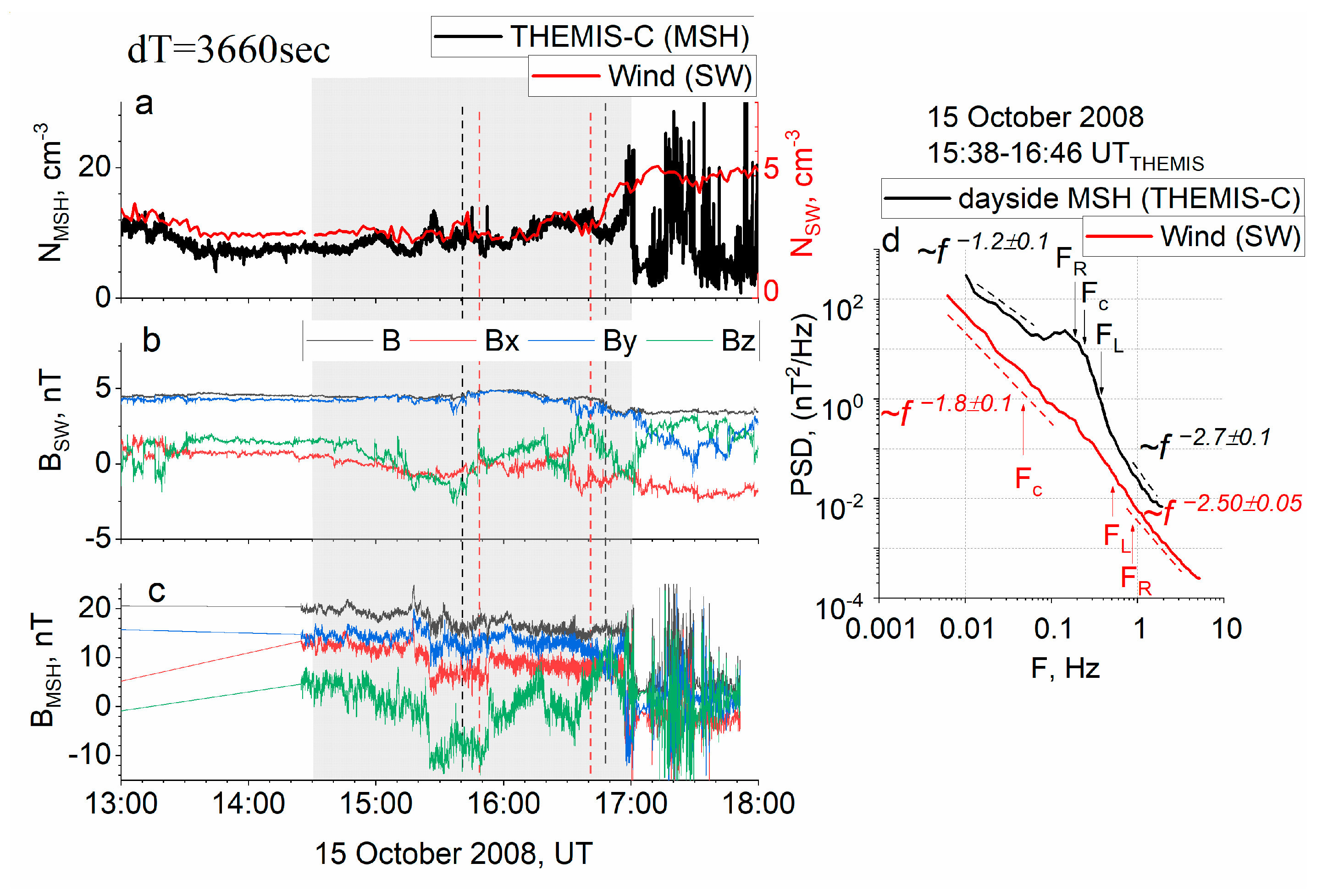
  • Interaction of any type of the SW with the quasi-perpendicular BS results in the modification of the turbulence properties at the MHD scales in the dayside MSH; the spectra in this region are substantially flatter than those observed in the SW and predicted for the developed turbulence;
  • At the kinetic scales, the spectra of magnetic field fluctuations may either become steeper at the quasi-perpendicular BS or stay unchanged; scaling at the frequencies above the ion spectral break is preserved in fast SW streams and in the CIR regions; the ICMEs are characterized by the most significant steepening in the dayside MSH;
  • Distinct SW regimes are accompanied by different ways of spectra modification during plasma tailward propagation; the MHD-scale properties of spectra restore for the Fast and CIR streams and stay slightly changed for Slow SW and ICMEs.
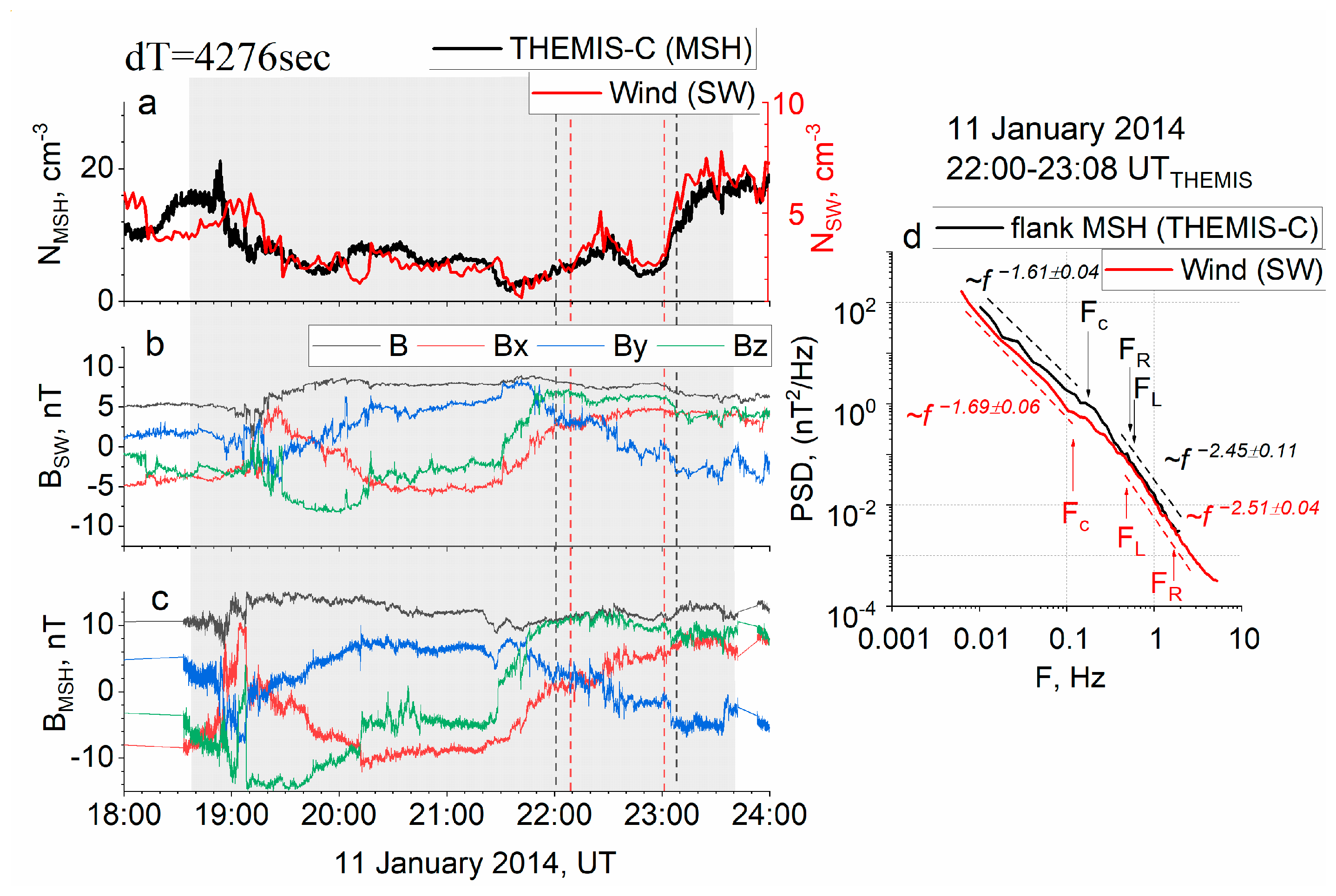
  • The kinetic-scale properties of the spectra for Slow and Fast SW at the MSH flanks are similar to those observed in the SW; ICME streams are characterized by a slightly steeper spectrum at the flanks, while compressed CIR flows exhibit a slight flattening at the kinetic scales.
The results demonstrate that the modification of f−5/3 scaling at the BS is the typical feature of the dayside MSH despite the differences in the flow properties in the SW. However, the modification of the scaling at the kinetic scales and the way of the scaling restoration at the flanks depend on the SW source at the Sun. This difference is suggested to be related to the differences in the geoefficiency of distinct SW flows. Fast SW and CIR regions attributed typically to the coronal holes exhibit the fewest changes in turbulence properties inside the MSH.

Author Contributions

Conceptualization, L.R. and M.R; methodology, L.R. and A.K.; software, L.R. and A.K.; validation, L.R., M.R. and G.Z.; writing—original draft preparation, L.R.; writing—review and editing, M.R.; visualization, L.R.; supervision, Y.Y. All authors have read and agreed to the published version of the manuscript.

Funding

This research was funded by RUSSIAN SCIENCE FOUNDATION, grant number 22-72-00105.

Data Availability Statement

Wind and THEMIS data can be found at https://cdaweb.gsfc.nasa.gov/ (accessed on 1 December 2023); catalog of large-scale solar wind types is available at http://iki.rssi.ru/pub/omni/catalog/ (accessed on 1 December 2023).

Conflicts of Interest

The authors declare no conflicts of interest.

References

  1. Borovsky, J.E.; Denton, M.H. The differences between CME-driven storms and CIR-driven storms. J. Geophys. Res. 2006, 111, A07S08. [Google Scholar] [CrossRef]
  2. Denton, M.H.; Borovsky, J.E.; Skoug, R.M.; Thomsen, M.F.; Lavraud, B.; Henderson, M.G.; McPherron, R.L.; Zhang, J.C.; Liemohn, M.W. Geomagnetic storms driven by ICME- and CIR-dominated solar wind. J. Geophys. Res. 2006, 111, A07S07. [Google Scholar] [CrossRef]
  3. Pulkkinen, T.I.; Goodrich, C.C.; Lyon, J.G. Solar wind electric field driving of magnetospheric activity: Is it velocity or magnetic field? Geophys. Res. Lett. 2007, 34, L21101. [Google Scholar] [CrossRef]
  4. Lavraud, B.; Borovsky, J.E. Altered solar wind-magnetosphere interaction at low Mach numbers: Coronal mass ejections. J. Geophys. Res. 2008, 113, A00B08. [Google Scholar] [CrossRef]
  5. Yermolaev, Y.I.; Nikolaeva, N.S.; Lodkina, I.G.; Yermolaev, M.Y. Specific interplanetary conditions for CIR-induced, Sheath-induced, and ICME-induced geomagnetic storms obtained by double superposed epoch analysis. Ann. Geophys. 2010, 28, 2177–2186. [Google Scholar] [CrossRef]
  6. Carbone, F.; Telloni, D.; Yordanova, E.; Sorriso-Valvo, L. Modulation of SolarWind Impact on the Earth’s Magnetosphere during the Solar Cycle. Universe 2022, 8, 330. [Google Scholar] [CrossRef]
  7. Podladchikova, T.V.; Petrukovich, A.A. Extended geomagnetic storm forecast ahead of available solar wind measurements. Space Weather. 2012, 10, S07001. [Google Scholar] [CrossRef]
  8. Boynton, R.J.; Balikhin, M.A.; Billings, S.A.; Sharma, A.S.; Amariutei, O.A. Data derived NARMAX Dst model. Ann. Geophys. 2012, 29, 965–971. [Google Scholar] [CrossRef]
  9. Zastenker, G.; Nozdrachev, M.; Němeček, Z.; Šafránková, J.; Paularena, K.; Richardson, J.; Lepping, R.; Mukai, T. Multispacecraft measurements of plasma and magnetic field variations in the magnetosheath: Comparison with Spreiter models and motion of the structures. Planet. Space Sci. 2002, 50, 601–612. [Google Scholar] [CrossRef]
  10. Hayosh, M.; Šafránková, J.; Němeček, Z. MHD-modelling of the magnetosheath ion plasma flow and magnetic field and their comparison with experiments. Adv. Space Res. 2006, 37, 507–514. [Google Scholar] [CrossRef]
  11. Hietala, H.; Partamies, N.; Laitinen, T.V.; Clausen, L.B.N.; Facskó, G.; Vaivads, A.; Koskinen, H.E.J.; Dandouras, I.; Rème, H.; Lucek, E.A. Supermagnetosonic subsolar magnetosheath jets and their effects: From the solar wind to the ionospheric convection. Ann. Geophys. 2012, 30, 33–48. [Google Scholar]
  12. Dmitriev, A.V.; Lalchand, B.; Ghosh, S. Mechanisms and Evolution of Geoeffective Large-Scale Plasma Jets in the Magnetosheath. Universe 2021, 7, 152. [Google Scholar] [CrossRef]
  13. Rakhmanova, L.; Riazantseva, M.; Zastenker, G. Correlation level between solar wind and magnetosheath plasma and magnetic field parameters. Adv. Space Res. 2016, 58, 157–165. [Google Scholar] [CrossRef]
  14. Pulkkinen, T.I.; Dimmock, A.P.; Lakka, A.; Osmane, A.; Kilpua, E.; Myllys, M.; Tanskanen, E.I.; Viljanen, A. Magnetosheath control of solar wind–magnetosphere coupling efficiency. J. Geophys. Res. Space Phys. 2016, 121, 8728–8739. [Google Scholar] [CrossRef]
  15. Šafránková, J.; Hayosh, M.; Gutynska, O.; Němeček, Z.; Přech, L. Reliability of prediction of the magnetosheath Bz component from interplanetary magnetic field observations. J. Geophys. Res. Space Phys. 2009, 114, A12213. [Google Scholar] [CrossRef]
  16. Pulinets, M.S.; Antonova, E.E.; Riazantseva, M.O.; Znatkova, S.S.; Kirpichev, I.P. Comparison of the magnetic field before the subsolar magnetopause with the magnetic field in the solar wind before the bow shock. Adv. Space Res. 2014, 54, 604–616. [Google Scholar] [CrossRef]
  17. Turc, L.; Fontaine, D.; Escoubet, C.P.; Kilpua, E.K.J.; Dimmock, A.P. Statistical study of the alteration of the magnetic structure of magnetic clouds in the Earth’s magnetosheath. J. Geophys. Res. Space Phys. 2017, 122, 2956–2972. [Google Scholar] [CrossRef]
  18. Alexandrova, O.; Chen, C.H.K.; Sorriso-Valvo, L.; Horbury, T.S.; Bale, S.D. Solar wind turbulence and the role of ion instabilities. Space Sci. Rev. 2013, 178, 101–139. [Google Scholar] [CrossRef]
  19. Bruno, R.; Carbone, V. The Solar Wind as a Turbulence Laboratory. Living Rev. Sol. Phys. 2013, 10, 2. [Google Scholar] [CrossRef]
  20. Zimbardo, G.; Greco, A.; Sorriso-Valvo, L.; Perri, S.; Vörös, Z.; Aburjania, G.; Chargazia, K.; Alexandrova, O. Magnetic turbulence in the geospace environment. Space Sci. Rev. 2010, 156, 89–134. [Google Scholar] [CrossRef]
  21. Huang, S.Y.; Hadid, L.Z.; Sahraoui, F.; Yuan, Z.G.; Deng, X.H. On the existence of the Kolmogorov inertial range in the terrestrial magnetosheath turbulence. Astrophys. J. Lett. 2017, 836, L10. [Google Scholar] [CrossRef]
  22. Rakhmanova, L.S.; Riazantseva, M.O.; Zastenker, G.N.; Verigin, M.I. Effect of the magnetopause and bow shock on characteristics of plasma turbulence in the Earth’s magnetosheath. Geomagn. Aeron. 2018, 58, 718–727. [Google Scholar] [CrossRef]
  23. Li, H.; Jiang, W.; Wang, C.; Verscharen, D.; Zeng, C.; Russell, C.T.; Giles, B.; Burch, J.L. Evolution of the Earth’s magnetosheath turbulence: A statistical study based on MMS observations. Astrophys. J. 2020, 898, L43. [Google Scholar] [CrossRef]
  24. Rakhmanova, L.; Riazantseva, M.; Zastenker, G.; Yermolaev, Y. Large-scale solar wind phenomena affecting the turbulent cascade evolution behind the quasi-perpendicular bow shock. Universe 2022, 8, 611. [Google Scholar] [CrossRef]
  25. Rakhmanova, L.; Riazantseva, M.; Zastenker, G.; Yermolaev, Y.; Lodkina, I. Dynamics of plasma turbulence at Earth’s bow shock and through the magnetosheath. Astrophys. J. 2020, 901, 30. [Google Scholar] [CrossRef]
  26. Rakhmanova, L.; Riazantseva, M.; Zastenker, G.; Verigin, M. Kinetic scale ion flux fluctuations behind the quasi-parallel and quasi-perpendicular bow shock. J. Geophys. Res. Space Phys. 2018, 123, 5300–5314. [Google Scholar] [CrossRef]
  27. Breuillard, H.; Matteini, L.; Argall, M.R.; Sahraoui, F.; Andriopoulou, M.; Le Contel, O.; Retinò, A.; Mirioni, L.; Huang, S.Y.; Gershman, D.J.; et al. New insights into the nature of turbulence in the Earth’s magnetosheath using magnetospheric multiscale mission data. Astrophys. J. 2018, 859, 127. [Google Scholar] [CrossRef]
  28. Yordanova, E.; Vörös, Z.; Raptis, S.; Karlsson, T. Current sheet statistics in the magnetosheath. Front. Astron. Space Sci. 2020, 7, 2. [Google Scholar] [CrossRef]
  29. Plank, J.; Gingell, I.L. Intermittency at Earth’s bow shock: Measures of turbulence in quasi-parallel and quasi-perpendicular shocks. Phys. Plasmas 2023, 30, 082906. [Google Scholar] [CrossRef]
  30. Gurchumelia, A.; Sorriso-Valvo, L.; Burgess, D.; Yordanova, E.; Elbakidze, K.; Kharshiladze, O.; Kvaratskhelia, D. Comparing quasi-parallel and quasi-perpendicular configuration in the terrestrial magnetosheath: Multifractal analysis. Front. Phys. 2022, 10, 903632. [Google Scholar] [CrossRef]
  31. Angelopoulos, V. The THEMIS mission. Space Sci. Rev. 2008, 141, 5–34. [Google Scholar] [CrossRef]
  32. McFadden, J.P.; Carlson, C.W.; Larson, D.; Ludlam, M.; Abiad, R.; Elliott, B.; Turin, P.; Marckwordt, M.; Angelopoulos, V. The THEMIS ESA plasma instrument and in-flight calibration. Space Sci. Rev. 2008, 141, 277–302. [Google Scholar] [CrossRef]
  33. Auster, H.U.; Glassmeier, K.H.; Magnes, W.; Aydogar, O.; Baumjohann, W.; Constantinescu, D.; Fischer, D.; Fornacon, K.H.; Georgescu, E.; Harvey, P.; et al. The THEMIS Fluxgate Magnetometer. Space Sci. Rev. 2008, 141, 235–264. [Google Scholar] [CrossRef]
  34. Yermolaev, Y.I.; Nikolaeva, N.S.; Lodkina, I.G.; Yermolaev, M.Y. Catalog of large-scale solar wind phenomena during 1976–2000. Cosm. Res. 2009, 47, 81–94. [Google Scholar] [CrossRef]
  35. Shevyrev, N.N.; Zastenker, G.N. Some features of the plasma flow in the magnetosheath behind quasi-parallel and quasi-perpendicular bow shocks. Planet. Space Sci. 2005, 53, 95–102. [Google Scholar] [CrossRef]
  36. Spreiter, J.R.; Summers, A.L.; Alksne, A.Y. Hydromagnetic flow around the magnetosphere. Planet. Space Sci. 1966, 14, 223–250, IN1–IN2, 251–253. [Google Scholar] [CrossRef]
  37. Karlsson, T.; Raptis, S.; Trollvik, H.; Nilsson, H. Classifying the Magnetosheath Behind the Quasi-Parallel and Quasi-Perpendicular Bow Shock by Local Measurements. J. Geophys. Res. Space Phys. 2021, 126, e2021JA029269. [Google Scholar] [CrossRef]
  38. Koller, F.; Raptis, S.; Temmer, M.; Karlsson, T. The Effect of Fast Solar Wind on Ion Distribution Downstream of Earth’s Bow Shock. Astrophys. J. Lett. 2024, 964, L5. [Google Scholar] [CrossRef]
  39. Case, N.A.; Wild, J.A. A statistical comparison of solar wind propagation delays derived from multispacecraft techniques. J. Geophys. Res. Space Phys. 2012, 117, A2. [Google Scholar] [CrossRef]
  40. Ogilvie, K.W.; Chornay, D.J.; Fritzenreiter, R.J.; Hunsaker, F.; Keller, J.; Lobell, J.; Miller, G.; Scudder, J.D.; Sittler, E.C.; Torbert, R.B.; et al. SWE, a comprehensive plasma instrument for the Wind spacecraft. Space Sci. Rev. 1995, 71, 55–77. [Google Scholar] [CrossRef]
  41. Lepping, R.P.; Acũna, M.H.; Burlaga, L.F.; Farrell, W.M.; Slavin, J.A.; Schatten, K.H.; Mariani, F.; Ness, N.F.; Neubauer, F.M.; Whang, Y.C.; et al. The WIND magnetic field investigation. Space Sci. Rev. 1995, 71, 207–229. [Google Scholar] [CrossRef]
  42. Šafránková, J.; Němeček, Z.; Němec, F.; Přech, L.; Piňta, A.; Chen, C.H.K.; Zastenker, G.N. Solar wind density spectra around the ion spectral break. Astrophys. J. 2015, 803, 107. [Google Scholar] [CrossRef]
  43. Markovskii, S.A.; Vasquez, B.; Smith, C. Statistical Analysis of the High-Frequency Spectral Break of the Solar Wind Turbulence at 1 AU. Astrophys. J. 2008, 675, 1576. [Google Scholar] [CrossRef]
  44. Chen, C.H.K.; Leung, L.; Boldyrev, S.; Maruca, B.A.; Bale, S.D. Ion-scale spectral break of solar wind turbulence at high and low beta. Geophys. Res. Lett. 2014, 41, 8081–8088. [Google Scholar] [CrossRef] [PubMed]
  45. Woodham, L.D.; Wicks, R.T.; Verscharen, D.; Owen, C.J. The Role of Proton Cyclotron Resonance as a Dissipation Mechanism in Solar Wind Turbulence: A Statistical Study at Ion-kinetic Scales. Astrophys. J. 2018, 856, 49. [Google Scholar] [CrossRef]
  46. Smith, C.; Hamilton, K.; Vasquez, B.; Leamon, R. Dependence of the dissipation range spectrum of interplanetary magnetic fluctuations on the rate of energy cascade. Astrophys. J. 2006, 645, L85–L88. [Google Scholar] [CrossRef]
  47. Sahraoui, F.; Huang, S.Y.; Belmont, G.; Goldstein, M.L.; Rétino, A.; Robert, P.; De Patoul, J. Scaling of the electron dissipation range of solar wind turbulence. Astrophys. J. 2013, 777, 15. [Google Scholar] [CrossRef]
  48. Šafránková, J.; Němeček, Z.; Němec, F.; Verscharen, D.; Chen, C.H.K.; Ďurovcová, T.; Riazantseva, M. Scale-dependent Polarization of Solar Wind Velocity Fluctuations at the Inertial and Kinetic Scales. Astrophys. J. 2019, 870, 40. [Google Scholar] [CrossRef]
  49. Alexandrova, O. Solar wind vs magnetosheath turbulence and Alfvén vortices. Nonlinear Process. Geophys. 2008, 15, 95–108. [Google Scholar] [CrossRef]
  50. Boldyrev, S.; Perez, J.C. Spectrum of kinetic alfven turbulence. Astrophys. J. Lett. 2012, 758, 5. [Google Scholar] [CrossRef]
  51. Goldreich, P.; Sridhar, S. Toward a theory of interstellar turbulence. II. Strong alfvenic turbulence. Astrophys. J. 1995, 438, 763. [Google Scholar] [CrossRef]
  52. Taylor, G.I. The spectrum of turbulence. Proc. R. Soc. A Math. Phys. Eng. Sci. 1938, 164, 476–490. [Google Scholar] [CrossRef]
  53. Klein, K.G.; Howes, G.G.; Tenbarge, J.M. The violation of the taylor hypothesis in measurements of solar wind turbulence. Astrophys. J. Lett. 2014, 790, 20. [Google Scholar] [CrossRef]
  54. Mangeney, A.; Lacombe, C.; Maksimovic, M.; Samsonov, A.A.; Cornilleau-Wehrlin, N.; Harvey, C.C.; Bosqued, J.-M.; Trávníček, P. Cluster observations in the magnetosheath. Part 1: Anisotropies of the wave vector distribution of the turbulence at electron scales. Ann. Geophys. 2006, 24, 3507–3521. [Google Scholar] [CrossRef]
  55. Borovsky, J.E.; Denton, M.H.; Smith, C.W. Some properties of the solar wind turbulence at 1 AU statistically examined in the different types of solar wind plasma. J. Geophys. Res. Space Phys. 2019, 124, 2406–2424. [Google Scholar] [CrossRef]
  56. Bruno, R.; Trenchi, L.; Telloni, D. Spectral slope variation at proton scales from fast to slow solar wind. Astrophys. J. Lett. 2014, 793, L15. [Google Scholar] [CrossRef]
  57. Riazantseva, M.O.; Rakhmanova, L.S.; Yermolaev, Y.I.; Lodkina, I.G.; Zastenker, G.N.; Chesalin, L.S. Characteristics of Turbulent Solar Wind Flow in Plasma Compression Regions. Cosm. Res. 2020, 58, 468–477. [Google Scholar] [CrossRef]
  58. Pitňa, A.; Šafránková, J.; Němeček, Z.; Goncharov, O.; Němec, F.; Přech, L.; Chen, C.H.K.; Zastenker, G.N. Density fluctuations upstream and downstream of interplanetary shocks. Astrophys. J. 2016, 819, 41. [Google Scholar] [CrossRef]
  59. Alexandrova, O.; Mangeney, A.; Maksimovic, M.; Cornilleau-Wehrlin, N.; Bosqued, J.-M.; André, M. Alfvén vortex filaments observed in magnetosheath downstream of a quasiperpendicular bow shock. J. Geophys. Res. 2006, 111, A12208. [Google Scholar] [CrossRef]
  60. D’Amicis, R.; Telloni, D.; Bruno, R. The Effect of Solar-Wind Turbulence on magnetospheric Activity. Front. Phys. 2020, 8, 604857. [Google Scholar] [CrossRef]
  61. D’Amicis, R.; Perrone, D.; Velli, M.; Sorriso-Valvo, L.; Telloni, D.; Bruno, R.; De Marco, R. Investigating Alfvénic Turbulence in Fast and Slow Solar Wind Streams. Universe 2022, 8, 352. [Google Scholar] [CrossRef]
Figure 1. THEMIS positions during MSH crossings and corresponding SW types.
Universe 10 00194 g001
Figure 2. Example of the case on 15 October 2008: (a) ion density in the SW (red line) and in the MSH (black line); (b) IMF magnitude and components measured by Wind; (c) magnetic field components and magnitude measured by THEMIS-C in the MSH, the SW data are shifted in time by 3660 s; (d) magnetic field fluctuation spectra registered in the SW (red line) and in the MSH (black line).
Universe 10 00194 g002
Figure 4. Mean values of the slope P1 at the MHD scales (top panel) and slope P2 at the kinetic scales (bottom panel) in the SW, dayside MSH, and at the flank MSH for five considered SW types; symbols are shifted slightly along abscise axis for each location for easier comparison.
Universe 10 00194 g004
Figure 5. Distributions of the spectra slope changes at the MHD scales ΔP1 in the dayside MSH and at the flanks for different types of the SW: (a) ΔP1 distribution in the dayside MSH for Slow, ICME and CIR; (b) ΔP1 distribution in the dayside MSH for Slow, Fast and HCS; (c) ΔP1 distribution at the flanks for Slow, ICME and CIR; (b) ΔP1 distribution at the flanks for Slow, Fast and HCS.
Universe 10 00194 g005
Figure 6. Distributions of the spectra slope changes at the kinetic scales ΔP2 in the dayside MSH and at the flanks for different types of the SW: (a) ΔPc distribution in the dayside MSH for Slow, ICME and CIR; (b) ΔP2 distribution in the dayside MSH for Slow, Fast and HCS; (c) ΔP2 distribution at the flanks for Slow, ICME and CIR; (b) ΔP2 distribution at the flanks for Slow, Fast and HCS.
Universe 10 00194 g006
Table 1. Mean and median values and standard deviations for distributions of ΔP1 and ΔP2 in the dayside MSH and at flanks.
Scale RangeLocationParameterSlowFastHCSICMECIR
MHDDayside MSHmean−0.30−0.30−0.37−0.35−0.27
median−0.29−0.32−0.37−0.38−0.27
std0.210.200.200.250.16
Flank MSHmean−0.17−0.10−0.17−0.07
median−0.18−0.07−0.24−0.07
std0.230.20 0.220.20
KineticDayside MSHmean0.26−0.050.160.30.04
median0.25−0.070.140.320.01
std0.210.190.150.30.26
Flank MSHmean−0.01−0.030.08−0.08
median−0.06−0.040.03−0.13
std0.190.21 0.200.17
Disclaimer/Publisher’s Note: The statements, opinions and data contained in all publications are solely those of the individual author(s) and contributor(s) and not of MDPI and/or the editor(s). MDPI and/or the editor(s) disclaim responsibility for any injury to people or property resulting from any ideas, methods, instructions or products referred to in the content.

