
Non-Commutative Classical and Quantum Fractionary Cosmology: FRW Case

1
Department of Physics, Division of Science and Engineering, University of Guanajuato, Campus León, León 37150, Mexico
2
Department of Electrical Engineering, Engineering Division Campus Irapuato-Salamanca, University of Guanajuato, Salamanca 36885, Mexico
3
National Polytechnic Institute, Unidad Profesional Interdisciplinaria de Ingeniería Campus Hidalgo IPN (UPIIH), Carretera Pachuca—Actopan Kilometer 1+500, SanAgustín Tlaxiaca, Hidalgo 42162, Mexico
*
Author to whom correspondence should be addressed.
†
These authors contributed equally to this work.
Universe 2024, 10(5), 192; https://0-doi-org.brum.beds.ac.uk/10.3390/universe10050192
Submission received: 20 March 2024
/
Revised: 14 April 2024
/
Accepted: 23 April 2024
/
Published: 25 April 2024
(This article belongs to the Special Issue Recent Advances in Quantum Cosmology)
Abstract
:In this work, we will explore the effects of non-commutativity in fractional classical and quantum schemes using the flat Friedmann–Robertson–Walker (FRW) cosmological model coupled to a scalar field in the K-essence formalism. In previous work, we have obtained the commutative solutions in both regimes in the fractional framework. Here, we introduce non-commutative variables, considering that all minisuperspace variables do not commute, so the symplectic structure was modified. In the quantum regime, the probability density presents a new structure in the scalar field corresponding to the value of the non-commutative parameter, in the sense that this probability density undergoes a shift back to the direction of the scale factor, causing classical evolution to arise earlier than in the commutative world.
1. Introduction
The study and applications of fractional calculus (FC) to cosmology is a new line of research that was born approximately twenty years ago. We have recently worked along this line in the theory of K-essence and in the analysis of the K-essence theory, we find several relevant indicators for its study. When this theory is analyzed as a perfect fluid and in particular the barotropic parameter is constant, it is generally demonstrated that this theory is equivalent to General Relativity coupled to ordinary matter with a barotropic equation of state [1], which has been verified in particular with the standard FRW model [2] and an anisotropic model, the Bianchi type I. The second indicator and the one relevant for our case is that this is the only theory that when quantized under the ADM formalism, a fractional Wheeler–DeWitt equation (WDW) in the scalar field component is naturally obtained in different stages of the universe [2]. There are possibly complementary theories such as quasi-quintessence that could have the same behaviors given that they have a certain similarity with our approach; we will try to analyze them in the immediate future [3,4]. However, we have not found any work in the literature, where the idea of non-commutativity (NC) is applied to this formalism, which is why we are interested in studying the effects of NC variables from the fractional calculus approach and seeing their effects on the exact solutions or mathematical structure of the same. It is well known that there are various ways to introduce non-commutativity in the phase space and that they produce different dynamical systems from the same Lagrangian [5], as can be shown, for example, in reference [6] and references cited therein. Therefore, distinct choices for the NC algebra among the brackets render distinct dynamic systems. We will use non-commutativity in the coordinate space, which is where we have some working practice in the past, leaving the application of moments space for the future [7], where other quantities such as angular momentum appear between coordinates and momenta [8,9].
Usually, K-essence models coupled with gravity are restricted to the Lagrangian density of the form [1,10,11,12,13]
where R is the scalar of curvature, the canonical kinetic energy is given by , is an arbitrary function of the scalar field , and g is the determinant of the metric. K-essence was originally proposed as a model for inflation, and then as a model for dark energy, along with explorations of unifying dark energy and dark matter. During the development of research in non-commutative formalism within fractional cosmology in K-essence theory, the presence of non-commutativity that usually accompanied the term of the scale factor is disrupted here, since essentially Non-commutativity is more present in the scalar field, modifying the mathematical structure that usually occurs in works in this direction in non-fractional formalisms.
Then, the field equations are given by
where we have assumed the units with and, as usual, the semicolon means a covariant derivative, and the subscript X denotes differentiation with respect to X.
The same set of Equation (2a,b) is obtained if we consider the scalar field as part of the matter content, to say with the corresponding energy-momentum tensor
Also, considering the energy-momentum tensor of a barotropic perfect fluid,
with being the four-velocity satisfying the relation , the energy density, and P the pressure of the fluid. For simplicity, we consider a comoving perfect fluid. The pressure and energy density corresponding to the energy momentum tensor of the field X are
thus, the barotropic parameter for the equivalent fluid is
Notice that the case of a constant barotropic index (with the exception when ) can be obtained by the function
Choosing the barotropic parameter as
where the parameter
is relevant in our approach. Thus, we can write the barotropic parameter in terms of , when . With this, we can write the states in the evolution of our universe as:
We construct the Lagrangian and Hamiltonian densities for the plane FLRW cosmological model, considering a barotropic perfect fluid for the scalar field in the variable X, and present the general case for commutative formalism in Section 2 and non-commutative formalism in Section 3. We present the quantum version in both cases, in Section 4 and Section 5, respectively. Finally, Section 6 is devoted to discussions.
2. Commutative Fractional Classical Exact Solution
We start with the following classical Lagrangian density that comes from the flat Friedmann–Robertson–Walker fractionary cosmological model coupled to a scalar field in the K-essence formalism [2]
Using the standard definition of the momenta , where , we obtain
and introducing them into the Lagrangian density, we obtain the canonical Lagrangian as
Performing the variation with respect to the lapse function N, , the Hamiltonian constraint is obtained, where the classical density is written as
For simplicity, we work in the gauge , and in the following we use the reduced Hamiltonian density,
In previous work [2], we found that the barotropic parameter in K-essence theory has the form , and the fractional parameter is , so, when , then , and when , then . This is relevant because in the quantum regime, the Laplace transform of a fractional differential equation depends on the parameter (integer part of the fractional parameter).
With this, the Hamiltonian density is rewritten as
then, the Hamilton equations are
Substituting these results in the Hamiltonian constraint, we have that
where is an integration constant and . With this and using Equation (17), the solution for the scale factor becomes,
and the solution for the scalar field is
3. Non-Commutative Fractional Classical Exact Solution
We start with the following classical Hamiltonian that comes from the flat Friedmann–Robertson–Walker fractionary cosmological model coupled to a scalar field in the K-essence formalism (16), written in terms of the fractional parameter , and in particular gauge where to find the commutative equation of motion; we use the classical phase space variables , where the Poisson algebra for these minisuperspace variables are
In the commutative model, the solutions to the Hamiltonian equations are the same as in General Relativity, modified only by the fractional parameter. Now, the natural extension is to consider the non-commutativity version of our model, with the idea of non-commutativity between the two variables , so we apply a deformation of the Poisson algebra. For this, we start with the usual Hamiltonian (16), but the symplectic structure is modified as follows
where ★ is the Moyal product [14], and the resulting Hamiltonian density is
but the symplectic structure is the one that we know, the commutative one (24). It is well known that there are two formalisms to study concerning the non-commutative equations of motion; the first formalism that we exposed has the original variables, but with the modified symplectic structure,
and for the second formalism, we use the shifted variables (Bopp shift approach) but with the original (commutative) symplectic structure
In both approaches, we have the same result.
The commutation relations (24) can be implemented in terms of the commuting coordinates of the standard quantum mechanics (Bopp shift) and this results in a modification of the potential like term of the Hamiltonian density and one possibility is, for example,
These transformations are not the most general possible to define non-commutative fields. With this in mind, our Hamiltonian density has the form
the Hamilton equations are
with these equations, the solution for is the same as in the commutative case, so the solution for the scale factor becomes
where is the solution presented in Equation (22). The solution for the scalar field is related to as ; then
for both commutative solutions, the scale factor y scalar field are obtained when the non-commutative parameter goes to zero.
4. Commutative Fractional Quantum Exact Solution
The Wheeler–DeWitt (WDW) equation for this model is obtained by making the usual substitution into (16) and promoting the classical Hamiltonian density in the differential operator applied to the wave function , . Then, we have
For simplicity, the factor may be the factor ordered with in many ways. Hartle and Hawking [15] suggested what might be called semi-general factor ordering, which, in this case, would order the terms as , where Q is any real constant that measures the ambiguity in the factor ordering in the variables and its corresponding momenta.
Thus, Equation (37) is rewritten as
By employing the separation variables method for the wave function , we have the following two differential equations for
where considers the sign in the differential equation. The fractional differential Equation (40) can be given in the fractional frameworks, following [16] and identifying where now is the order of the fractional derivative taking values in ; then, we can write
the solution of Equation (41) with a positive sign may be obtained by applying direct and inverse Laplace transforms [16], providing
In the ordinary case, ; then, the solution is
Following the book of Polyanin [17] (page 179.10), we discovered the solution for the first equation for , considering different values in the factor ordering parameter and both signs in the constant ,
with order , where we had written the second expression in terms of the fractional order , and the solutions which become dependent on the sign of its argument; when (for ), the Bessel function becomes the ordinary Bessel function . When (for ), this becomes the modified Bessel function . For the particular values (), it will be necessary to solve the original differential equation for this variable.
Then, we have the probability density by considering only , ,
We will now report the solution for the case, which we have not reported before, considering the minus sign in the constant ; the general solution for the function becomes
and for the other sign , it becomes
and the corresponding solutions to (41) for both signs are
so, the probability density becomes
On the other hand, it is well known that in the standard quantum cosmology, the wave function is un-normalized. There is no systematic method to do this, as the Hamiltonian density is not Hermitian. In particular cases, wave packets can be constructed, and from these wave packets, we can construct a normalized wave function. In this work, we could not construct these wave packets. We hope to be able to do this in future studies.
5. Non-Commutative Fractional Quantum Exact Solution
As already mentioned, we are looking for the non-commutative deformation of the flat FRW quantum cosmological model. In order to find the non-commutative generalization, we need to solve the non-commutative Einstein equation; this is a formidable task due to the highly non-linear character of the theory; fortunately, we can circumvent these difficulties by following Ref. [18].
Now, we can proceed to the non-commutative model; we will consider that the minisuperspace variables do not commute, so that the symplectic structure is modified as follows
In particular, we choose the following representation
where the parameters are a measure of the non-commutativity between the minisuperspace variables. The commutation relations (50) or (51) are not the most general ones for defining a non-commutative field.
We consider the non-commutative Hamiltonian density in a simple way, as
It is well known that this non-commutativity can be formulated in terms of non-commutative minisuperspace functions with the Moyal star product ★ of functions. The commutation relations (50) can be implemented in terms of the commuting coordinates of the standard quantum mechanics (Bopp shift) and this results in a modification of the potential-like term of the WDW equation [18,19], and one possibility is, for example,
These transformations are not the most general possible for defining non-commutative fields. However, these shifts modify the potential term in the following way
As in the commutative case, we choose the wave function to be separable, , obtaining
which can be rewritten as
If we want this equation to be separable, we must choose to make the term within the square parentheses [ ] a constant, in particular ; with this choice, we retrieve the commutative quantum equation for the function , (39), with the same quantum solution (44).
At this point, we want to note that in commutative quantum cosmology, the prefactor that accompanies its moments is not contemplated when we use a particular gauge, and usually the non-commutative parameter enters the solution of the function, not that of the scalar field . In this case, the appearance of the prefactor in fractional cosmology makes the solution in remain the same, but not the part of the scalar field, where the non-commutative parameter appears and the mathematical structure is completely different.
That said, the expression (56) becomes
Since the non-commutative parameter is very small, we can stay until the first term in this one, obtaining
In this fractional differential equation, when we recover the commutative equation for the quantum function (40). Now, we solve Equation (58) written as follows
where . For the particular value , we can observe that Equation (52) becomes the ordinary commutative quantum equation; then, the quantum solutions, commutative and non-commutative, are the same in this approach to K-essence theory.
However, in the dust scenario . Equation (59) takes the form
whose solution is given by
Thus, the probability density becomes (considering only the real part of the complex exponential in )
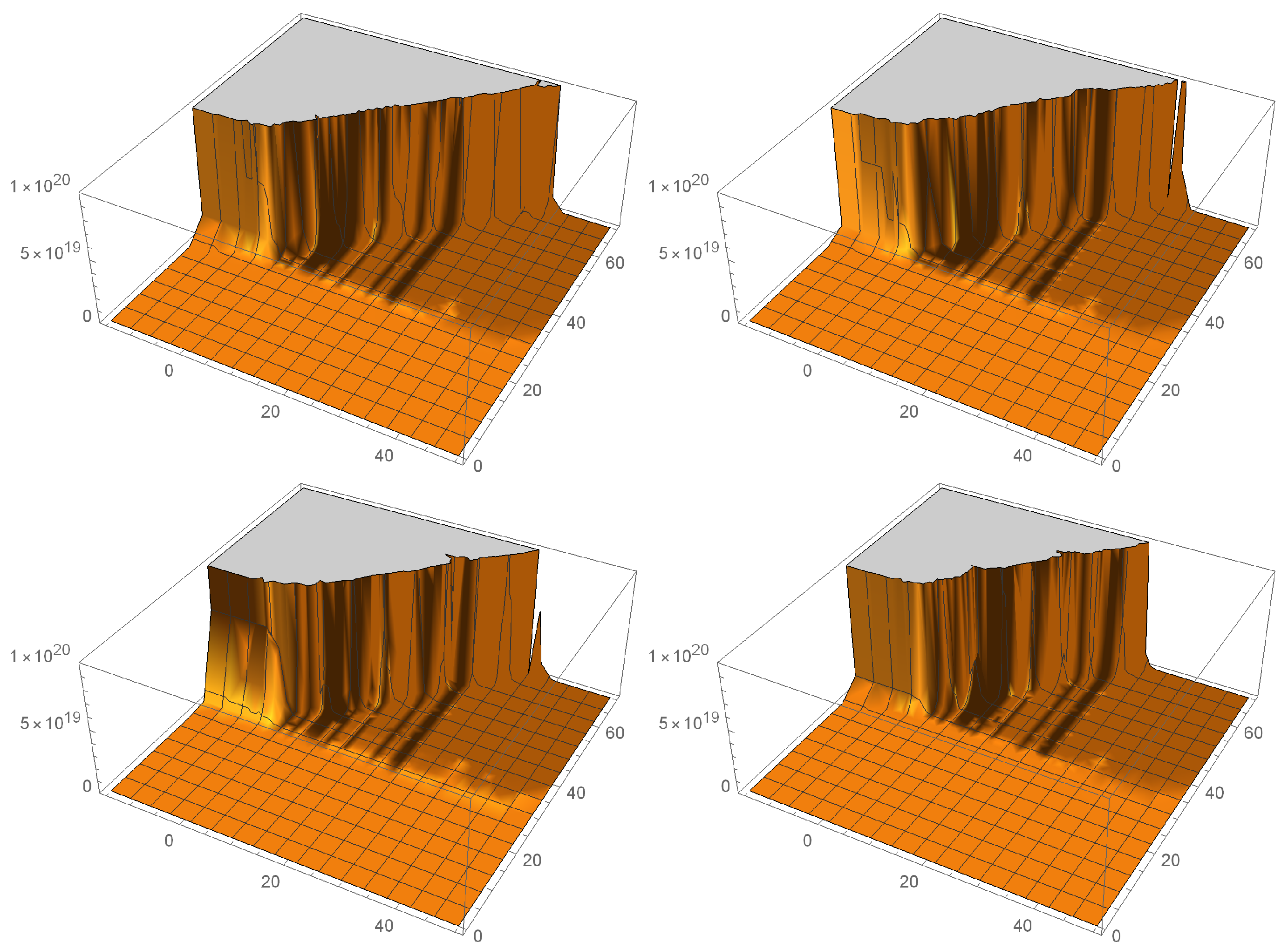
To make Figure 1, we use the ordinary Bessel function. We can see the effect of the combination of the parameters and , where the probability density undergoes a shift in the behavior of the scalar field, at the beginning and at the end, that is, modifying the structure. As we can see, at , a crack appears; at , it separates and a peak appears; at , the peak decreases and disappears at , when 5. However, the fact that some peaks no longer appear does not mean that they have been canceled, but rather that, due to the change in probability density, the scales of these peaks are no longer on the graph. This pattern is repeated when the factor ordering parameters are ; that is why we do not introduce these graphs.
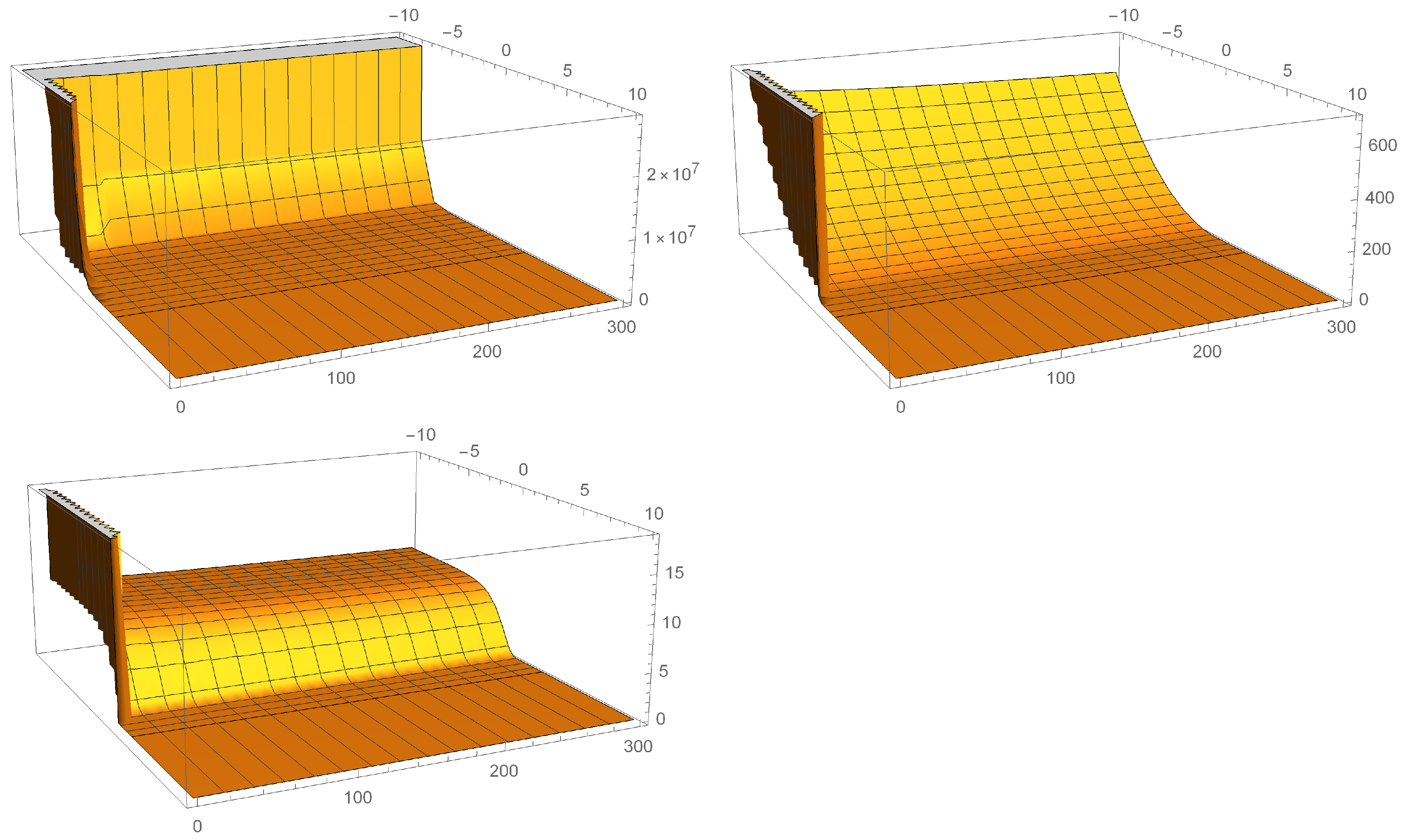
For the other scenarios, employing the modified Bessel function, the behavior is very different, as shown in Figure 2, Figure 3 and Figure 4, when the combination of the parameters and has decaying behavior in the direction of the evolution of the scale factor like () and oscillatory behavior in the direction of the scalar field, or making the scalar field relevant in quantum evolution and remaining in classical evolution, as has been found in other alternative models to Einstein’s theory [20].
Since we do not know the initial conditions of the universe in the dust epoch, we have graphed both probability densities, where it is observed that the scalar field persists in the evolution of both densities, remaining as a remnant towards the classical evolution of the universe, being a cosmic background currently.
The global effect of the non-commutativity between the field coordinates of the system in the fractional quantum cosmology scheme causes the probability density to shift or shrink in the opposite direction to the scale factor, causing the classical universe to emerge sooner, which would mean that the current universe should have more time than is usually mentioned, as mentioned in reference [21], employing the fractional framework.
On the other hand, if the order of the differential Equation (59) is rational, then solutions have two cases.
5.1. , ,
Taking into account the Laplace transform in [16], considering that , , and , then let the fractional differential equation
where
Applying the Laplace transform to all the terms in (63), we have
Solving with respect to , we obtain
For the particular value , the two last terms can be considered as one, making , and for , the first and last term can be simplified to
From the formula in [16] (page 40, equation (3.11) with a correction), we have
adapting our parameters to the master Equation (67), we have the following three cases
- For the first term in (66), we use , ,
- For the second term in (66), we use , ,
- For the third term in (66), we use , ,
Then, the inverse Laplace transform of (66) is
For the case when and , , we see that the complex solution can be read as
where and .
5.2. , ,
For this case, the equation to solve is
Similarly, as in the previous case, we have
which can be rewritten as
with this, we write the probability density for this case as
In the following, we present the quantum behavior to post-inflation-like case , then , taking the value in the non-commutative parameter for different values in the factor ordering parameter . In Figure 5, it can be observed that in a very small interval in the evolution of the scalar field, the probability density presents a mountain, which fades in the direction of the scalar field to a constant plateau. The behavior of the constant plateau for this stage of the universe was found in the commutative part in paper [2] using the Mittag–Leffler functions; now, they are obtained under this solution in power series of the scalar field and the modified Bessel functions of the case.
6. Discussion
During the development of research in non-commutative formalism within fractional cosmology in K-essence theory, the presence of non-commutativity that usually accompanied the term of the scale factor here is disrupted, since essentially non-commutativity is more present in the scalar field, modifying the mathematical structure that usually occurs in works in this direction in non-fractional formalisms.
In our non-commutative quantum development, the method of separation of variables does not appear in a traditional way as the sum of the operators in their variables; now, it is produced as factors; thanks to this, it can be separated; in addition, now complex fractional differential equations arise, even in cases with derivatives of integer order, which means that these solutions in the scalar field have a real part and an imaginary part.
In previous non-commutative quantum work [7], the term is usually modified with the scale factor, but in fractional cosmology in K-essence, this term remains unchanged, only the scalar field term undergoes important modifications, in the sense that the probability density undergoes a shift back to the direction of the scale factor, causing classical evolution to arise earlier than in the commutative world. This effect is due to the non-commutativity between the field coordinates in this formalism, which is related to some crucial effects due to the fact of having a fractional equation, such that the age of the universe is greater, of the order of 13.8196 Gyr., or more [21]. Recently, another age of our universe was found using fractional geometric parameter and thermodynamics variables, that being 13.91 Gyr. [22]. Although these authors use a different formalism than ours, we consider that something can be done using different methods, such as the one proposed in a previous work by one of the authors of this work [23]. These results on fractal K-essence theory add to the fact that this formalism without considering ordinary matter is falsified with this approach according to the classical solutions that are identical using the FRW model [2], but it is found that this is a more general result mentioned in reference [1].
Since the prefactor that is usually linked to the ordering of the factors under a certain gauge does not appear in the standard quantum Hamiltonian, the important contribution of non-commutativity appears in the wave function linked to the scale factors, which is why this term continues to persist. This causes the momentum associated with the scalar field to produce an additional total derivative term to the non-commutative fractional equation due to the Bopp shift in the scale factor term, producing in this case a significant contribution of the non-commutative parameter in the wave function; see Equation (59).
This methodology can be replicated to the Bianchi type I anisotropic model, where up to six non-commutative parameters appear, and possibly to the Bianchi Class A, results that will be reported at another time.
Author Contributions
Conceptualization, J.S., J.J.R. and L.T.-S.; methodology, J.S., J.J.R. and L.T.-S.; software, J.S. and L.T.-S.; validation, J.S., J.J.R. and L.T.-S.; formal analysis, J.S., J.J.R. and L.T.-S.; investigation, J.S., J.J.R. and L.T.-S.; writing—original draft preparation, J.S., J.J.R. and L.T.-S.; writing—review and editing, J.S., J.J.R. and L.T.-S.; visualization, J.S.; supervision, J.S. and J.J.R. All authors have read and agreed to the published version of the manuscript.
Funding
J.S. was partially supported by PROMEP grants UGTO-CA-3. Both authors were partially supported by SNI-CONACyT. J.J. Rosales is supported by the UGTO-CA-20 nonlinear photonics and Department of Electrical Engineering. L.T.S. is supported by Secretaria de Investigación y Posgrado del Instituto Politécnico Nacional, grant SIP20211444.
Data Availability Statement
No new data were created or anlyzed in this study. Date sharing is not applicable to this article.
Acknowledgments
This work is part of the collaboration within the Instituto Avanzado de Cosmología. Many calculations were done by Symbolic Program REDUCE 3.8.
Conflicts of Interest
The authors declare no conflicts of interest.
References
- Arroja, F.; Sasaki, M. Note on the equivalence of a barotropic perfect fluid with a k-essence scalar field. Phys. Rev. D 2010, 81, 107301. [Google Scholar] [CrossRef]
- Socorro, J.; Rosales, J.J. Quantum fractionary cosmology: K-essence theory. Universe 2023, 9, 185. [Google Scholar] [CrossRef]
- D’Agostino, R.; Luongo, O.; Muccino, M. Healing the cosmological constant problem during inflation through a unified quasi-quintessence matter field. Class. Quantum Gravity 2022, 39, 195014. [Google Scholar] [CrossRef]
- Luongo, O.; Mengoni, T. Quasi-quintessence inflation with non-minimal coupling to curvature in the Jordan and Einstein frames. arXiv 2023, arXiv:2309.03065. [Google Scholar]
- Abreu, E.M.C.; Neves, C.; Oliveira, W. Noncommutativity from the symplectic point of view. Int. J. Mod. Phys. A 2006, 21, 5359–5369. [Google Scholar] [CrossRef]
- Andrade, M.A.D.; Neves, C.J. Noncommutative Mapping from the symplectic formalism. Math. Phys. 2018, 59, 012105. [Google Scholar] [CrossRef]
- Guzman, W.; Sabido, M.; Socorro, J. On Noncommutative Minisuperspace and the Friedmann equations. Phys. Lett. B 2011, 697, 271–274. [Google Scholar] [CrossRef]
- López, J.L.; Sabido, M.; Yee-Romero, C. Phase space deformation in phantom cosmology. Phys. Dark Universe 2018, 19, 104–108. [Google Scholar] [CrossRef]
- Picón, J.L.L.; Sabido, M.; Yee-Romero, C. Phase space deformation in SUSY cosmology. Phys. Lett. B 2024, 849, 138420. [Google Scholar] [CrossRef]
- de Putter, R.; Linder, E.V. Kinetic k-essence and Quintessence. Astropart. Phys. 2007, 28, 263. [Google Scholar] [CrossRef]
- Chiba, T.; Dutta, S.; Scherrer, R.J. Slow-roll k-essence. Phys. Rev. D 2009, 80, 043517. [Google Scholar] [CrossRef]
- Bose, N.; Majumdar, A.S. A k-essence model of inflation, dark matter and dark energy. Phys. Rev. D 2009, 79, 103517. [Google Scholar] [CrossRef]
- García, L.A.; Tejeiro, J.M.; Castañeda, L. K-essence scalar field as dynamical dark energy. arXiv 2012, arXiv:1210.5259. [Google Scholar]
- Szabo, R.J. Quantum field theory on noncommutative spaces. Phys. Rep. 2003, 378, 207–299. [Google Scholar] [CrossRef]
- Hartle, J.B.; Hawking, S.W. Wave function of the Universe. Phys. Rev. D 1983, 28, 2960–2975. [Google Scholar] [CrossRef]
- Milici, C.; Drăgănescu, G.; Machado, J.T. Introduction to Fractional Differential Equations; Springer Nature: Cham, Switzerland, 2019. [Google Scholar]
- Polyanin, A.C.; Zaitsev, V.F. Handbook of Exact Solutions for Ordinary Differential Equations, 2nd ed.; Chapman & Hall/CRC: Boca Raton, FL, USA, 2003. [Google Scholar]
- Garcia-Compean, H.; Obregón, O.; Ramírez, C. Noncommutative quantum cosmology. Phys. Rev. Lett. 2002, 88, 161301. [Google Scholar] [CrossRef] [PubMed]
- Pimentel, L.O.; Mora, C. Noncommutative quantum cosmology. Gen. Relativ. Gravit. 2005, 37, 817–821. [Google Scholar] [CrossRef]
- Socorro, J.; Pérez-Payán, S.; Hernández-Jiménez, R.; Espinoza-García, A.; Díaz-Barrón, L.R. Classical and quantum exact solutions for a FRW in chiral like cosmology. Class. Quantum Gravity 2021, 38, 135027. [Google Scholar] [CrossRef]
- Costa, E.W.d.; Jalalzadeh, R.; Júnior, P.F.d.; Rasouli, S.M.M.; Jalalzadeh, S. Estimated Age of the Universe in Fractional Cosmology. Fractal Fract. 2023, 7, 854. [Google Scholar] [CrossRef]
- Jalalzadeh, R.; Jalalzadeh, S.; Jahromi, A.S.; Moradpour, H. Friedmann equations of the fractal apparent horizon. Phys. Dark Universe 2024, 44, 101498. [Google Scholar] [CrossRef]
- Omar, E.; Núñez, O.E.N.; Socorro, J.; Hernández-Jiménez, R. Hamilton’s approach in cosmological inflation with an exponential potential and its observational constraints. Astrophys. Space Sci. 2019, 364, 69. [Google Scholar]
Figure 1.
In the following plots, we show the behavior of the probability density of Equation (62), considering the sign in , taking the values , and , respectively.
Figure 1.
In the following plots, we show the behavior of the probability density of Equation (62), considering the sign in , taking the values , and , respectively.

Figure 2.
In the following plots, we show the behavior of the probability density of Equation (62), considering the sign in , taking the values , and , respectively.
Figure 2.
In the following plots, we show the behavior of the probability density of Equation (62), considering the sign in , taking the values , and , respectively.

Figure 3.
In the following plots, we show the behavior of the probability density of Equation (62), considering the sign in , taking the values , and , respectively.
Figure 3.
In the following plots, we show the behavior of the probability density of Equation (62), considering the sign in , taking the values , and , respectively.

Figure 4.
In the following plots, we show the behavior of the probability density of Equation (62), considering the sign in , taking the values , and , respectively.
Figure 4.
In the following plots, we show the behavior of the probability density of Equation (62), considering the sign in , taking the values , and , respectively.

Figure 5.
In the post-inflation-like scenario , which corresponds to or in Equation (76), for ; from top to bottom, respectively, we consider the value for the parameter and . In these graphs, we use the only and the modified Bessel function.
Figure 5.
In the post-inflation-like scenario , which corresponds to or in Equation (76), for ; from top to bottom, respectively, we consider the value for the parameter and . In these graphs, we use the only and the modified Bessel function.

Disclaimer/Publisher’s Note: The statements, opinions and data contained in all publications are solely those of the individual author(s) and contributor(s) and not of MDPI and/or the editor(s). MDPI and/or the editor(s) disclaim responsibility for any injury to people or property resulting from any ideas, methods, instructions or products referred to in the content. |
© 2024 by the authors. Licensee MDPI, Basel, Switzerland. This article is an open access article distributed under the terms and conditions of the Creative Commons Attribution (CC BY) license (https://creativecommons.org/licenses/by/4.0/).
Share and Cite
MDPI and ACS Style
Socorro, J.; Rosales, J.J.; Toledo-Sesma, L. Non-Commutative Classical and Quantum Fractionary Cosmology: FRW Case. Universe 2024, 10, 192. https://0-doi-org.brum.beds.ac.uk/10.3390/universe10050192
AMA Style
Socorro J, Rosales JJ, Toledo-Sesma L. Non-Commutative Classical and Quantum Fractionary Cosmology: FRW Case. Universe. 2024; 10(5):192. https://0-doi-org.brum.beds.ac.uk/10.3390/universe10050192
Chicago/Turabian StyleSocorro, J., J. Juan Rosales, and Leonel Toledo-Sesma. 2024. "Non-Commutative Classical and Quantum Fractionary Cosmology: FRW Case" Universe 10, no. 5: 192. https://0-doi-org.brum.beds.ac.uk/10.3390/universe10050192
Note that from the first issue of 2016, this journal uses article numbers instead of page numbers. See further details here.