

Measurement and Assessment of Reactive, Unbalanced and Harmonic Line Losses


Power Electronics Laboratory, School of Electrical Engineering, Sichuan University, Chengdu 610065, China
*
Author to whom correspondence should be addressed.
Electronics 2024, 13(9), 1680; https://0-doi-org.brum.beds.ac.uk/10.3390/electronics13091680
Submission received: 1 March 2024
/
Revised: 11 April 2024
/
Accepted: 23 April 2024
/
Published: 26 April 2024
Abstract
:This study investigates the feasibility of utilizing the line loss power factor to assess the reactive, unbalanced, and harmonic line losses in low-voltage distribution networks and explores the method of calculating decoupled line loss values based on this factor. To achieve this objective, we establish preliminary definitions of single-phase and three-phase reactive, unbalanced, and harmonic line loss power factors, drawing upon the principles of electrical theory outlined in IEEE Standard 1459. These power factors serve as crucial indicators for evaluating the severity of line losses caused by reactive power, unbalance, and harmonic problems. Subsequently, the values of line loss attributed to reactive, unbalanced, and harmonic components are decoupled and quantified using the line loss power factor as a fundamental parameter. The effectiveness and accuracy of the proposed method were verified in Matlab simulation and physical experiments.
1. Introduction
The proliferation of non-linear power loads in power systems has been observed alongside the expanding scale of power consumption, necessitating the resolution of corresponding power quality issues [1,2,3]. Notably, China’s low-voltage distribution network incurs a significant proportion amounting to 60% of the total power supply and distribution network loss, as evidenced by relevant statistical data [4]. This directly impacts the economic benefits of power grid enterprises [5,6]. There are many causes of power quality problems, such as voltage fluctuations, flicker, transient overvoltage, reactive power, harmonics, three-phase imbalance, etc., of which reactive power, harmonics, and three-phase imbalance have a very obvious impact on the grid line loss. They are the key factors leading to a significant increase in line loss [7]. When there is a slight power quality loss in the line, the cost of governing the line may not be justified. To maximize the input–output ratio, reactive, unbalanced, and harmonic line loss assessment indicators can be used as criteria for deciding whether governance is necessary or not. Consequently, achieving precise computation and assessment of line loss components assumes paramount significance in promoting improvements in electric energy conservation and loss reduction endeavors.
The line loss study of distribution networks can be categorized into two main areas: (1) Theoretical line loss calculation research. This line loss research primarily employs accurate modeling to simulate line operations and calculate line loss. The quantitative investigation of theoretical line loss involves the precise determination of line resistance values. For example, in reference [8], the calculation of a power distribution network under harmonic influence was studied, where transmission line AC coefficients and transformer harmonic loss were introduced to construct line models. Reference [9] examined a line harmonic loss model considering the skin effect. This model provides more accurate calculations of harmonic loss compared to traditional models. Reference [10] proposed a theoretical line loss computation approach via matrix completion and a ReliefF-convolutional neural network (CNN) for LVDN. Reference [11] proposed a continuous line loss calculation method for the distribution network with higher calculation accuracy. Reference [12] proposed an optimized distributed generation allocation method aimed at minimizing total losses in distribution systems, while reference [13] introduced a novel approach to calculate line loss under three-phase imbalance conditions. However, these studies only address single power quality issues and cannot be applied to composite power quality problems. Considering the effects of composite power quality, reference [14] proposed a composite power quality loss model for a 10 kV distribution grid, considering harmonics, unbalanced three-phase currents, and voltage deviations. The FLUKE 435 Power Quality and Energy Analyzer can separate line currents, input line resistance, and subsequently calculate individual component line loss. Nevertheless, accurately determining harmonic resistance values is challenging due to the skin effect and proximity under harmonic conditions, which can cause significant deviations in line loss calculations using the decoupled line loss calculation method of the FLUKE 435 Power Quality and Energy Analyzer, lacking practical application guidance. Meanwhile, in the actual working conditions of the low-voltage distribution network, measuring the line length accurately is usually challenging. As a result, the calculated line impedance based on the line length may have a certain degree of error.
(2) Statistical line loss calculation research. Statistical line loss research obtains relevant data by subtracting electricity sales data from electricity input data. Statistical line loss calculations avoid the need to determine equivalent line resistances. However, the decoupling of bus losses cannot be accomplished utilizing the conventional technique of utilizing the meter data from the primary end of the transformer outlet line meter minus the meter data from the client side of the meter at the conclusion of all branches, via the conventional power theory. Additionally, most research on statistical line loss calculations is qualitative, with limited quantitative studies on the impact of composite power energy quality. Reference [15] examined the differences between theoretical line loss and statistical line loss and analyzed the causes of these discrepancies. Reference [16] investigated the sources of error that affect the accuracy of statistical line loss data. In addition to this, references [17,18,19] conducted corresponding studies considering the main factors affecting line losses and methods to reduce them. In summary, it is vital to consider quantitative line loss calculations for composite power quality in low-voltage distribution networks.
Accurate measurement, calculation, and assessment of line loss are essential for making informed decisions regarding line management and loss reduction measures. This study is based on the aforementioned research foundation and proposes a methodology for deriving power quality line loss values without the need to solve for equivalent resistances. The paper begins by defining four types of power quality line loss power factors, based on the power theory outlined in IEEE Std. 1459 [20,21,22,23]. The IEEE Std. 1459 is underpinned by Emanuel power theory [20] and encompasses both sinusoidal and non-sinusoidal situations, as well as balanced and unbalanced states. Notably, this power theory introduces the concept of “equivalent”, wherein a fully compensating system is employed to replace the actual line and load. This equivalent system exhibits a perfectly sinusoidal positive sequence current, with the neutral line current being zero. The power loss in this hypothetical system matches the actual power loss that generates the same thermal stress. This concept provides a theoretical foundation for conducting line loss research based on IEEE Std. 1459. The IEEE Working Group is in the process of improving the IEEE 1459 standard considering the physical meaning of the measurement theory and reactive power definitions [24,25], but this does not affect the application of the IEEE 1459 standard in line loss calculations and line loss analyses, due to the fact that the line loss itself is caused by the current flowing through the line.
The power decomposition for both single-phase and three-phase systems is depicted in Table 1. The four power quality line loss power factors based on the power decomposition are defined in Table 1.
These power factors serve as evaluative metrics for assessing line loss in single-phase and three-phase systems under composite power quality problems. Furthermore, utilizing these power factors, this study deduces the line loss caused by reactive power problems, harmonic problems, and imbalance problems. It also calculates the ratio of the fundamental active line loss to the decoupled line loss values. To validate the proposed methodology, we conduct simulations using the Matlab/Simulink tool and perform physical experiments. An error analysis of the experimental results confirms the feasibility and accuracy of the theoretical derivation presented in this study, underscoring its potential as a practical guide for real-world applications.
2. Line Loss Power Factor Presentation
Line loss ∆PLoss refers to the power loss that occurs during the transmission of electric energy from the power source to the load through the transmission lines. When the power factor PF is equal to 1, the line loss is minimized. The minimum line loss ∆PLoss-min is obtained when PF = 1. ∆PLoss-min can be calculated using (2) by fully compensating for the non-active current, ensuring that the load current consists solely of an active current and the line transmits only active power. In (1) and (2), R is the line resistance, and U is the voltage at the first end of the line.
Based on the aforementioned analysis, the power factor PF can be calculated as depicted in (3) and (4).
Equation (4) provides the definition of power factor PF in terms of line loss, and, likewise, PF can be employed to evaluate line loss resulting from non-active power. The subsequent section elucidates the line loss power factor in the context of both single-phase and three-phase systems.
- A.
- Single-Phase Case
The model of transmission lines in power systems can be categorized into two types based on the length of the line: lumped-parameter equivalent model and distributed-parameter equivalent model. Low-voltage distribution lines, which are considered short lines, typically utilize lumped-parameter π-type equivalent circuit models, as illustrated in Figure 1.
Figure 1 depicts R as the equivalent resistance of the low-voltage distribution line, and X is the equivalent reactance.
The line loss in short lines can be approximately equal to the resistive power; hence, reactance and shunt admittance are disregarded in the analysis of line loss [9]. Figure 2 shows a schematic diagram for loss analysis in the single-phase low-voltage state [26]. In the figure, R represents the line resistance of the circuit in the low-voltage distribution network, while I denotes the current flowing through the line, and the voltage across the load is represented by U.
When a non-linear load is connected to the system, the current flowing through the single-phase non-sinusoidal system induces a line loss in the line resistance. To analyze this, voltage, current, and phase angle data are collected at Point 2. The original single-phase system is then transformed equivalently, and the load is measured by decomposing the apparent power S. The line loss can be expressed using (5).
In (5), the apparent power S is considered using IEEE Std. 1459, and the decomposition process is shown in Table 1. From (5), it is evident that all components of the apparent power S contribute to line loss. However, given the minimal voltage distortion in the line, the impact of voltage distortion power Du and harmonic apparent power SH in line loss can be disregarded. The total line loss ∆PLoss can be decomposed based on power quality problems into the following components, fundamental active line loss ∆PP-min, reactive additional line loss ∆PQ, and harmonic additional line loss ∆PH. It should be noted that only the fundamental active line loss ∆PP-min is attributed to the line itself, while the remaining components represent additional loss resulting from power quality factors.
To evaluate the quality of line loss and quantify the reactive additional line loss caused by reactive power and the harmonic additional line loss resulting from current distortion power, three power factors are defined for a single-phase system. These power factors, namely the active line loss power factor PFP, the reactive line loss power factor PFQ, and the harmonic line loss power factor PFH, are analogous to the single-phase fundamental power factor PF1. The definitions of power factor for the power quality of a single-phase system are presented below. In the following equations, SLoss denotes the total line loss apparent power, S1 denotes the fundamental apparent power, and SPH denotes the harmonic line loss apparent power.
The active line loss power factor PFP is employed to evaluate the quality of line loss by quantifying the contribution of fundamental active power P1 to the total line loss. Its value ranges between 0 and 1, reflecting the proportion of line loss attributed to the fundamental active power. A PFP value of 1 signifies the absence of additional line loss in the system due to power quality factors.
The reactive line loss power factor PFQ is utilized to assess the contribution of reactive power to the reactive additive line loss, ranging between 0 and 1. As the reactive additive line loss increases, the PFQ value decreases. A PFQ value of 1 indicates the absence of additional reactive line loss in the system.
The harmonic line loss power factor PFH is employed to assess the impact of a distorted current on the harmonic additive line loss. Its value ranges between 0 and 1 and decreases as the harmonic additive line loss increases. A PFH value of 1 indicates the absence of harmonic additional line loss in the system.
The power cubes of the active line loss power factor PFP, reactive line loss power factor PFQ, and harmonic line loss power factor PFH are presented in Figure 3. It represents the relationship between the decomposed individual powers on the vector.
- B.
- Three-Phase Case
The line loss analysis of the three-phase system of the low-voltage distribution network is carried out for the three-phase four-wire system, for example, according to Figure 4 for the three-phase four-wire system. Four lines of the same model are used in the analysis, ignoring the differences in the parameters of these four lines [9].
In Figure 4, R is the line resistance. When a non-linear load is connected to the system, the three-phase currents IA, IB, IC, and neutral current In produce line loss in the line resistance R. The three-phase voltage, current, and phase angle information at measurement Point 2 is collected, and the original three-phase system is equivalently transformed to decompose the load measurement equivalent apparent power Se [24,25]. The equivalent system has the same line power losses as the actual distribution system, and Figure 4 shows a schematic diagram of the three-phase, four-wire low-voltage distribution system after introducing the equivalence.
The total line loss ∆PeLoss can be represented by (7).
In (7), the load measurement equivalent apparent power Se is performed using IEEE Std. 1459, and the decomposition process is shown in Table 1. As observed from (7), each component of the equivalent apparent power Se contributes to line loss. These line losses can be further decomposed into the following components based on power quality issues, fundamental positive sequence active line loss ∆PeP-min, fundamental positive sequence reactive additional line loss ∆PeQ, unbalanced additional line loss ∆PeU, and harmonic additional line loss ∆PeH.
By drawing an analogy to the three-phase fundamental positive sequence power factor PF1+, the following power factors are defined for the three-phase system, the fundamental positive sequence active line loss power factor PFeP, the reactive line loss power factor PFeQ, the unbalanced line loss power factor PFeU, and the harmonic line loss power factor PFeH. The maximum value of these line loss power factors is 1. These factors for power line loss enable the assessment of line loss due to power quality issues in three-phase systems. In the following formulas, SeLoss denotes the total line loss apparent power, S1+ denotes the fundamental positive sequence apparent power, SePU denotes the unbalanced line loss apparent power, and SePH denotes the harmonic line loss apparent power.
The line loss power factors for a three-phase system serve as valuable metrics to evaluate the line loss. The values of the fundamental positive sequence active line loss power factor PFeP, the reactive line loss power factor PFeQ, the unbalanced line loss power factor PFeU, and the harmonic line loss power factor PFeH range between 0 and 1, diminishing as power-quality-related additional line losses increase. When there are no power quality-related additional line losses in the system, the values of all four line loss power factors are equal to 1.
3. Line Loss Ratio and Decoupling Presentation
The line loss power factor is a critical tool for evaluating the influence of power quality issues on line loss. Furthermore, it allows for the calculation of the ratio between power quality line loss and fundamental active line loss, aiding in the assessment of whether reactive power problems, harmonic problems, and imbalance problems need to be addressed. Additionally, it enables the decoupling of the values of different components of power quality line loss without the requirement to measure line loss resistance values.
- A.
- Single-Phase Case
In a single-phase system, the formulas for calculating the ratio between power quality line loss and fundamental active line loss are presented below.
This is because the fundamental active line loss represents the loss caused by the line itself. The power quality line loss ratio values can be utilized to assess whether the corresponding power quality problems need to be addressed.
Furthermore, the contribution of each line loss component can be separately determined using the single-phase line loss power factor and the difference in line losses ∆PLoss measured at Point 1 and Point 2 in the single-phase system diagram depicted in Figure 1. This decoupling process does not necessitate solving for line resistance values. The values for each decoupled line loss component can be calculated as follows.
By leveraging the active line loss power factor PFP, reactive line loss power factor PFQ, and harmonic line loss power factor PFH of a single-phase system, it is possible to decouple and analyze the total line loss. This approach allows for a comprehensive evaluation of the line loss associated with single-phase energy quality.
Line losses can also be calculated using the equivalent resistance method, i.e., as shown in (11), which is a commonly used method for calculating line losses.
The equivalent resistance method uses current and line resistance to make line loss measurements. Unfortunately, resistance measurement is a very difficult problem when there is a harmonic influence, and research has been slow to progress, which leads to large measurement errors in the resistance data when calculating line losses using the equivalent current method, which can affect the accuracy of the results [25]. In contrast, the use of the power quality line loss power factor to calculate line loss power is able to circumvent the measurement of resistance due to the influence of harmonics and, at the same time, convert small values of current and resistance measurements into large values of power measurements on the customer side, improving the accuracy of line loss calculations.
- B.
- Three-Phase Case
The calculation of the power quality line loss ratio and line loss decoupling for a three-phase system is analogous to that for a single-phase system, as demonstrated in the following equations. The line loss ∆PeLoss represents the discrepancy between active power measurements at Point 1 and Point 2 in Figure 4.
The decoupling of total line loss and the evaluation of three-phase power quality line loss are achieved through the utilization of base-wave positive sequence power factors, namely PFeP for active line loss, PFeQ for reactive line loss, PFeU for unbalanced line loss, and PFeH for harmonic line loss within the context of the three-phase system. This comprehensive approach allows for the disentanglement and accurate quantification of distinct components contributing to line loss, enabling a thorough analysis of power system performance and quality.
4. Indicator Characterization Simulation and Experimental Results
- A.
- Single-Phase Case Simulation Results
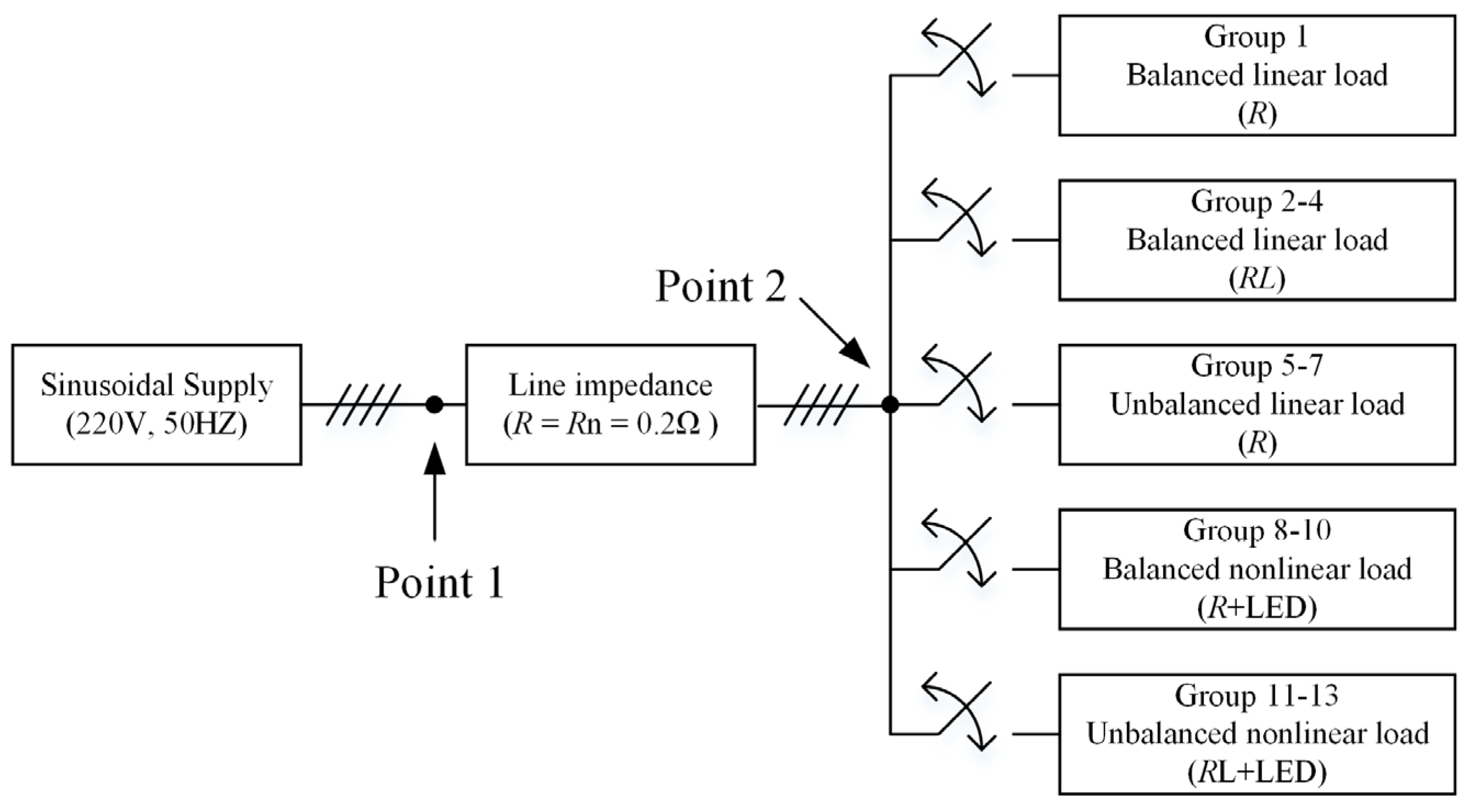
The proposed method underwent validation using a simplistic test system, as illustrated in Figure 5, to address the single-phase non-sinusoidal scenario. Among them, Group 1 is a perfect single-phase sinusoidal simulation group with a power factor of 1.0. Groups 2–4 are single-phase sinusoidal simulation groups with reactive power, current harmonic content THDI of 0%, and power factor gradually decreasing from 0.9 to 0.7 in steps of 0.1. Groups 5–7 are single-phase harmonic simulation groups with a power factor of 1.0, and current harmonic content THDI gradually increases from 10% to 30% in steps of 10%. Groups 8–10 are single-phase harmonic simulation groups with compound power quality problems. Simulink was employed to manipulate the reactive and harmonic power at varying levels, facilitating the simulation of different degrees of reactive and harmonic problem load groups, thereby emulating diverse system operation states.
The single-phase simulation system was configured with a rated frequency of 50 Hz for the single-phase AC supply, a voltage RMS of 220 V, and a phase angle of 0°. The line impedance Z was set to R = 0.2 Ω. The single-phase simulation model is shown in Figure 6.
The simulation model was created in the Simulink environment. The load used to simulate users consisted of linear load and LED. The load in Groups 1 to 4 only contains linear load, and the load in Groups 5 to 10 contains both linear load and LED, as shown in Figure 6. In the LED simulation model, capacitor C1 is set to 440 × 10−6 F, capacitor C2 is set to 200 × 10−5 F, and inductor L1 is set to 200 × 10−5 H. The settings of the Pulse Generator module, Mosfet module, and diode module are shown in Table 2. The varying degrees of power quality problems in the single-phase simulation model are realized by changing the value of R1 in the LED module and the RLC load. The load settings in Groups 1 to 10 are shown in Table 3.
Initially, three line loss power factors, i.e., active line loss power factor PFP, reactive line loss power factor PFQ, and harmonic line loss power factor PFH, are measured at Point 2 to evaluate the line loss of the single-phase simulated system and calculating the line loss percentage. The calculated results are also compared with the difference in power measured at the beginning and end of the line, i.e., the difference in power measured at Point 1 and Point 2.
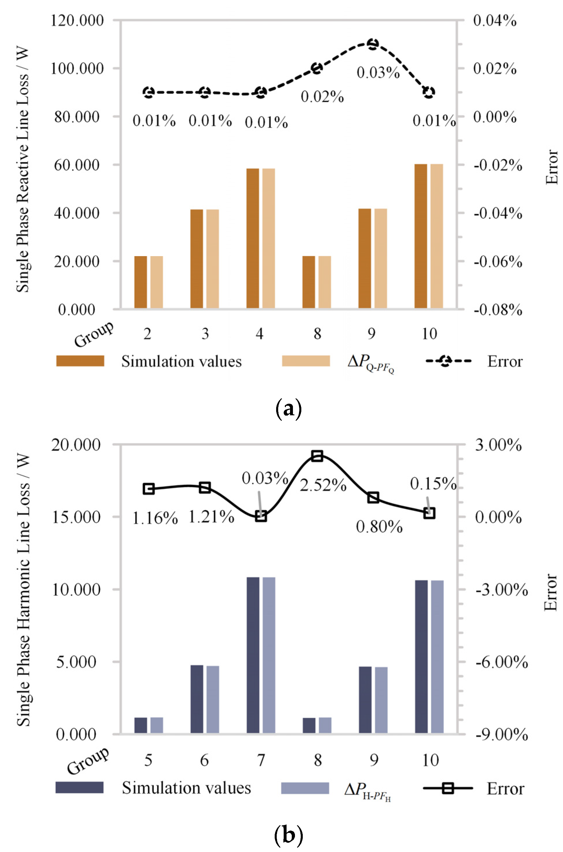
The simulation results of the single-phase system are shown in Table 4a,b and Figure 7 and Figure 8. Error/% in Table 4b indicates the error between the simulated and calculated values.
As can be seen from Table 4a,b and Figure 7, the decoupled power quality line loss errors and line loss percentage errors obtained using the three types of line loss power factors are very small. The errors of the 10 sets of simulation results are below 3%, and the calculated results obtained are very close to the simulated measurement results, which indicates that the method of calculating the line loss using the line loss power factor on the customer side is feasible.
As can be seen from Figure 8, when the system has no reactive and harmonic problems, i.e., in a “perfect” single-phase system, the active line power factor PFQ, the reactive line loss assessment index PFQ, and the harmonic line loss assessment index PFH are one; when the power factor Φ decreases and the current harmonic content ζ increases, the active line power factor PFP, the reactive line loss assessment index PFQ, and the harmonic line loss assessment index PFH are reduced. In addition, the three line loss assessment indicators can clearly characterize the severity of the system’s line loss caused by power quality problems, whether it is a single power quality problem or a compound power quality problem, which shows that it is feasible to use the three line loss power factors to assess the system’s power quality line loss.
- B.
- Three-Phase Case Simulation Results
The proposed method is validated using a simplistic three-phase test system, illustrated in Figure 9, to address a three-phase non-sinusoidal unbalanced scenario. There are 13 three-phase simulation groups, among which Group 1 is a perfect three-phase balanced sinusoidal simulation group with a power factor of 1.0. Groups 2–4 are three-phase balanced sinusoidal simulation groups with reactive power, and the power factor decreases gradually from 0.9 to 0.7 in steps of 0.1. Groups 5–7 are three-phase unbalanced sinusoidal simulation groups with a power factor of 1.0, and the degree of negative-sequence imbalance increases from 0.1 to 0.3 in steps of 0.1. Groups 8–10 are three-phase balanced harmonic simulation groups with a power factor of 1.0 and current harmonic content THDeI in steps of 10% increases from 10% to 30%. Groups 11–13 are three-phase unbalanced harmonic simulation groups, containing reactive power and compound power quality problems.
The three-phase simulation system was configured with a rated frequency of 50 Hz for the three-phase AC supply and an RMS voltage value of 220 V. The line impedance was set to R = Rn = 0.2 Ω. The three-phase simulation model is shown in Figure 10. The load settings in Groups 1 to 10 are shown in Table 5.
The simulation model was created in the Simulink environment, and the load used to simulate users consisted of a linear load and LED. The load in Groups 1 to 7 only contains linear load, and the load in Groups 8 to 13 contains both linear load and LED, as shown in Figure 10. The varying degrees of power quality problems in the three-phase simulation model are realized by changing the value of R1 in the LED module and the RLC load. In the LED simulation model for phase A, capacitor C1_A is set to 440 × 10−6 F, capacitor C2_A is set to 200 × 10−5 F, and inductor L1_A is set to 200 × 10−5 H. The settings of the Pulse Generator module, Mosfet module, and diode module for phase A are shown in Table 2. The LED module simulation settings for phase B and phase C are the same as for phase A.
Initially, four line loss power factors, i.e., fundamental positive sequence active line loss power factor PFeP, reactive line loss power factor PFeQ, unbalanced line loss power factor PFeU, and harmonic line loss power factor PFeH, are measured at Point 2 for evaluating the line loss of the three-phase simulated system and calculating the line loss percentage. The calculated results are also compared with the difference in power measured at the beginning and end of the line, i.e., the difference in power measured at Point 1 and Point 2.
The calculated results are also compared with the difference in power measured at the beginning and end of the line, i.e., the difference in power measured at Point 1 and Point 2. The results are shown in Table 6a,b and Figure 11 and Figure 12. The current spectra of the neutral line harmonic simulation data for Groups 8 to 13 are shown in Table 7.
As can be seen in Table 6a,b and Figure 11, compared to the simulated measured line loss values for the three-phase system, the error in the calculated line loss values for each component using the four line loss power factors is small, with the error in all 13 sets of simulated results not exceeding 2%, which indicates that it is theoretically feasible to calculate the additional line loss values for the decoupled power quality using the four line loss power factors.
As can be seen from Figure 12, when the system has no reactive, harmonic, and unbalance problems, i.e., in a “perfect” three-phase system, all four power quality line loss power factors are 1. When the power factor Φ decreases, the current harmonic content ζ increases and the unbalance ε increases, the fundamental positive sequence active line loss power factor PFeP, reactive line loss power factor PFeQ, unbalanced line loss power factor PFeU, and harmonic line loss power factor PFeH will decrease. Whether the system has a single power quality problem or a compound power quality problem, the line loss power factor is an effective way to assess the severity of the system’s power quality line loss problem.
- C.
- Three-Phase Case Experimental Results
In the simulation section, simulated single-phase and three-phase systems were employed to illustrate the theoretical viability of the line loss calculation using line power factors. Subsequently, an experiment involving a three-phase non-sinusoidal unbalanced system was established. The system was configured at 220 V for a low-voltage distribution network and was composed of linear RL loads along with LED light banks. The wiring diagram of the physical experiment is depicted in Figure 13. Comprehensive loads’ data can be found in Table 8.
In the physical experiment without power on, HIOKI IM 3536 LCR METER was used to measure the line resistance labelled as 10 Ω, and the result was 9.75 Ω. At the same time, in the line resistance at both ends of the parallel connection voltmeter, a series connection ammeter was used in the power supply to measure the harmonic effects of the line resistance of the voltage and current values, so as to calculate the consideration of the skin effect of the line resistance value of 9.99 Ω. These two resistance values are entered into FLUKE 435 to calculate the line loss value. Meanwhile, measurement points were established at both ends of the physical experimental line. At the initial end, a Fluke 438 Power Quality Analyzer was utilized, while at the terminal end, a Fluke 435 Power Quality and Energy Analyzer was employed. These meters simultaneously sampled voltage, current, and power values at the respective ends to ensure data synchronicity. The discrepancy between the two ends was considered the measured line loss value.
A comparison between the approach proposed in this study and the measurements obtained from FLUKE 435 is illustrated in Table 9a–d.
Table 9a shows the results of the active line loss experiment. In Table 9a, PFeP is 0.8738. True value-P represents the line loss of the positive sequence active current generated by the fundamental frequency, which is calculated by multiplying the difference between the positive sequence active power at the start and end of the line by the square of the sine of the phase angle of the positive sequence current.
When comparing the errors of the proposed method to the FLUKE 435 measurement method in this study, it is evident that the FLUKE 435 recorded the greatest error in the active line loss, which had a value of 7.587%, without taking skin effect into consideration. After accounting for the skin effect, the measurement error of the FLUKE 435 was reduced to a value of 4.845%. However, there is still a certain error with True value-P because it is impossible to measure the line loss on the conductor. The method proposed in this study produced the line loss value with the lowest error, at 0.490%.
Table 9b shows the results of the reactive line loss experiment. In Table 9b, the power factor Φ of the three-phase experimental circuit stands at 0.9984, and PFeQ is 0.9984. The line loss caused by the base-sequence reactive current is represented by True value-Q, which is calculated by multiplying the difference between the fundamental-sequence active power at the beginning and end of the line by the square of the cosine of the phase angle of the fundamental-sequence current. The line loss calculated by the method proposed in this paper has the smallest error, with a value of 0.490%, compared to the measurement results obtained from FLUKE 435.
Table 9c shows the results of the unbalanced line loss experiment. In Table 9c, the three-phase imbalance ε is 16.23%, and PFeQ is 0.9434. True value-U denotes the line loss of unbalanced current. It is calculated by subtracting the fundamental positive sequence active power from the fundamental active power at the beginning and end of the line. Our proposed method calculates the line loss value with a minimal error of 2.501% when compared to the measurements obtained from FLUKE 435.
Table 9d shows the results of the harmonic line loss experiment. In Table 9d, the negative sequence current manifests a harmonic content ζ of 40.32%, and PFeU is 0.9194. True value-H denotes the line loss due to harmonic currents, which is obtained by subtracting the harmonic active power from the first and last ends of the line. Compared with the FLUKE 435 measurements, the line loss value calculated by the proposed method in this paper has the smallest error, with a value of 1.065%.
From Table 9a–d, it can be observed that PFeQ, PFeU, and PFeH are 0.9984, 0.9434, and 0.9194, respectively. Notably, the values of these power quality line loss factors fall within a range of 0 to 1, all being below 1. This signifies that PFeQ, PFeU, and PFeH can effectively evaluate the system’s power quality line loss problem when line loss due to power quality problems is present. Concurrently, in comparison with line loss values calculated using Fluke 435, the line loss values computed through the power quality line loss power factor presented in this paper exhibit closer alignment with measured quantities and manifest smaller errors. This emphasizes the feasibility of employing the proposed power quality line loss power factor method for calculating and decoupling power quality line losses on the customer side.
In line loss measurement and analysis, using traditional power theory, i.e., the method of subtracting the first and last meters, can calculate the total loss of the line, but it is not possible to further decouple the total line loss; using Fluke 435 for measurement, it is necessary to manually enter the value of the line impedance, so as to decouple the total loss of the line, but the decoupled results have a certain degree of error compared with the actual line loss. Errors in the FLUKE 435 are mainly caused by errors in the value of the line resistance. Due to the presence of harmonics in the system, the skin effect and the collinear effect can cause changes in the resistance value, thus affecting the line resistance and the accurate measurement of the line loss value. The use of the line power factor enables the calculation of the power quality of each component without the need to solve for line resistance, thus effectively avoiding the errors caused by line resistance.
5. Conclusions
This work focuses on analyzing losses caused by reactive, unbalance, and harmonic issues in electrical lines and decoupling total line losses to quantify individual contributions. Based on IEEE Std. 1459 power theory, four line loss power factors are proposed to evaluate the severity of reactive, unbalance, and harmonic problems. These factors enable the calculation of decoupled line loss values for each line component without needing to solve for line resistance, given the total line loss is known.
Compared to traditional power theory, which relies on circuit impedance for line loss calculations, this method simplifies the process significantly. Measuring line impedance accurately is challenging and prone to errors. The proposed method avoids the need for impedance measurement altogether, shifting the focus to the direct measurement of line loss and utilizing end-of-line analysis for assessing power values on the user side. This approach provides essential metrics for line loss management and evaluation. It offers significant guidance for power grid companies aiming to reduce energy consumption and enhance economic efficiency.
This provides an overview of unbalanced compensation techniques using power electronic converters for active distribution systems with renewable generation.
Author Contributions
Conceptualization, Q.Z. and Y.D.; methodology, Q.Z. and Y.D.; software, Y.D.; validation, Y.D.; formal analysis, Y.D.; investigation, Y.D., C.C. and H.L.; resources, Q.Z. and Y.D.; data curation, Y.D.; writing—original draft preparation, Y.D.; writing—review and editing, Y.D.; visualization, Y.D.; supervision, Q.Z., X.L. and M.L.; project administration, Q.Z. All authors have read and agreed to the published version of the manuscript.
Funding
This research received no external funding.
Data Availability Statement
Data are contained within the article.
Conflicts of Interest
The authors declare no conflict of interest.
List of Symbols
| U | Voltage RMS (V) |
| U1 | Fundamental voltage RMS (V) |
| UH | Harmonic voltage RMS (V) |
| Ue | Equivalent voltage RMS (V) |
| Ue1 | Fundamental equivalent voltage RMS (V) |
| U1+ | Fundamental positive sequence voltage RMS (V) |
| UeH | Equivalent harmonic voltage RMS (V) |
| I | Current RMS (A) |
| I1 | Fundamental current RMS (A) |
| I1+ | Fundamental positive sequence current RMS (A) |
| I1- | Fundamental negative sequence current RMS (A) |
| IH | Harmonic current RMS (A) |
| Ie | Equivalent current RMS (A) |
| Ie1 | Fundamental equivalent current RMS (A) |
| IeH | Equivalent harmonic current RMS (A) |
| φ1 | Fundamental phase angle (°) |
| φ1+ | Fundamental positive sequence phase angle (°) |
| S | Apparent power (VA) |
| S1 | Fundamental apparent power (VA) |
| SN | Non-fundamental apparent power, (VA) |
| SH | Single-phase harmonic apparent power (VA) |
| Se | Equivalent apparent power (VA) |
| Se1 | Fundamental equivalent apparent power (VA) |
| S1+ | Fundamental positive sequence apparent power (VA) |
| SU1 | Unbalanced apparent power (VA) |
| SeN | Non-fundamental equivalent apparent power (VA) |
| SeH | Three-phase harmonic apparent power (VA) |
| SLoss | Single-phase total line loss apparent power (VA) |
| SPH | Single-phase harmonic line loss apparent power (VA) |
| SeLoss | Three-phase total line loss apparent power (VA) |
| SePU | Three-phase unbalanced line loss apparent power (VA) |
| SePH | Three--phase harmonic line loss apparent power (VA) |
| P | Active power (W) |
| P1 | Fundamental active power (W) |
| PH | Harmonic active power (W) |
| P1+ | Fundamental positive sequence active power (W) |
| ∆PLoss | Total line loss (W) |
| ∆PLoss-min | The minimum line loss (W) |
| ∆PP-min | Single-phase fundamental active line loss (W) |
| ∆PQ | Single-phase reactive additional line loss (W) |
| ∆PH | Single-phase harmonic additional line loss (W) |
| ∆PeLoss | Three-phase total line loss (W) |
| ∆PeP-min | Three-phase fundamental positive sequence active line loss (W) |
| ∆PeQ | Three-phase fundamental positive sequence reactive additional line loss (W) |
| ∆PeU | Three-phase unbalanced additional line loss (W) |
| ∆PeH | Three-phase harmonic additional line loss (W) |
| N | Non-active power (VAR) |
| Q1 | Fundamental reactive power (VAR) |
| DI | Current distortion power (VAR) |
| DU | Voltage distortion power (VAR) |
| Q1+ | Fundamental positive sequence reactive power (VAR) |
| DeI | Three-phase current distortion power (VAR) |
| DeU | Three-phase voltage distortion power (VAR) |
| R | Line equivalent resistance (Ω) |
| X | Line equivalent reactance (Ω) |
| Y | Line equivalent admittance (S) |
| PFP | Single-phase active line loss power factor |
| PFQ | Single-phase reactive line loss power factor |
| PFH | Single-phase harmonic line loss power factor |
| PFeP | Three-phase fundamental positive sequence active line loss power factor |
| PFeQ | Three-phase reactive line loss power factor |
| PFeU | Three-phase unbalanced line loss power factor |
| PFeH | Three-phase harmonic line loss power factor |
| Φ | Power Factor |
| ζ | THDI |
| ε | The degree of negative-sequence imbalance |
| U | Voltage RMS (V) |
References
- Fu, J.; Han, Y.; Li, W.; Feng, Y.; Zalhaf, A.S.; Zhou, S.; Yang, P.; Wang, C. A Novel Optimization Strategy for Line Loss Reduction in Distribution Networks with Large Penetration of Distributed Generation. Int. J. Electr. Power Energy Syst. 2023, 150, 109–112. [Google Scholar] [CrossRef]
- Rafi, F.H.M.; Hossain, M.J.; Rahman, S.M.; Taghizadeh, S. An Overview of Unbalance Compensation Techniques Using Power Electronic Converters for Active Distribution Systems with Renewable Generation. Renew. Sustain. Energy Rev. 2020, 125, 109812. [Google Scholar] [CrossRef]
- Antić, T.; Thurner, L.; Capuder, T.; Pavić, I. Modeling and Open Source Implementation of Balanced and Unbalanced Harmonic Analysis in Radial Distribution Networks. Electr. Power Syst. Res. 2022, 209, 107935. [Google Scholar] [CrossRef]
- Zhang, J. Study on the Mechanism of Power Quality Disturbance Affecting Distribution Network Loss. Master’s Thesis, Department of Electrical Engineering, North China Electric Power University, Beijing, China, 2019. [Google Scholar]
- Suliman, M.S.; Hizam, H.; Othman, M.L. Determining Penetration Limit of Central PVDG Topology Considering the Stochastic Behaviour of PV Generation and Loads to Reduce Power Losses and Improve Voltage Profiles. IET Renew. Power Gener. 2020, 14, 2629–2638. [Google Scholar] [CrossRef]
- Wu, H.; Dong, P.; Liu, M. Distribution Network Reconfiguration for Loss Reduction and Voltage Stability with Random Fuzzy Uncertainties of Renewable Energy Generation and Load. IEEE Trans. Ind. Inform. 2020, 16, 5655–5666. [Google Scholar] [CrossRef]
- Feng, C.; Xu, C.; Li, H. Analysis of Three Phase Current Unbalance and Harmonic Influence on Power Loss. Electr. Appl. 2016, 35, 47–52. [Google Scholar]
- Wei, C.; Li, Q.; Jiang, J. Quantification calculation and modeling simulation of distribution network losses considering harmonic factor. J. Zhengzhou Univ. (Eng. Sci.) 2018, 39, 53–58+66. [Google Scholar]
- Wang, Y.; Liu, S.; Li, Q. Parameter identification and experimental verification of harmonic resistance loss model in low-voltage distribution lines. Power Syst. Technol. 2021, 45, 1480–1486. [Google Scholar]
- Liu, R.; Pan, F.; Yang, Y.; Hong, W.; Li, Q.; Lin, K.; Liu, S. Theoretical Line Loss Calculation Method for Low-Voltage Distribution Network via Matrix Completion and ReliefF-CNN. Energy Rep. 2023, 9, 1908–1916. [Google Scholar] [CrossRef]
- Li, Y.; Ma, X.; Liang, C.; Li, Y.; Cai, Z.; Jiang, T. Continuous Line Loss Calculation Method for Distribution Network Considering Collected Data of Different Densities. Energies 2022, 15, 5171. [Google Scholar] [CrossRef]
- Mahmoud, K.; Yorino, N.; Ahmed, A. Optimal Distributed Generation Allocation in Distribution Systems for Loss Minimization. IEEE Trans. Power Syst. 2016, 31, 960–969. [Google Scholar] [CrossRef]
- Hao, S.; Cai, X.; Zhang, Y. Quantitative analysis of three-phase unbalance and line loss. Power Syst. Technol. 2020, 45, 1547–1552. [Google Scholar]
- Li, Q.; Liu, S.; Wen, J. Calculation model of 10 kV distribution network loss considering power quality impact and its experimental verification. Electr. Power Autom. Equip. 2022, 42, 212–220. [Google Scholar]
- Xie, W.; Zhang, C.; Cao, J. Difference between statistical line loss and theoretical line loss in line loss delicacy project. East China Electr. Power 2009, 37, 13–16. [Google Scholar]
- Tang, D.; Li, J.; Meng, Z. Research on accuracy of statistical line losses. Power Syst. Prot. Control. 2009, 46, 33–39. [Google Scholar]
- Moghaddam, M.J.H.; Kalam, A.; Shi, J.; Nowdeh, S.A.; Gandoman, F.H.; Ahmadi, A. A New Model for Reconfiguration and Distributed Generation Allocation in Distribution Network Considering Power Quality Indices and Network Losses. IEEE Syst. J. 2020, 14, 3530–3538. [Google Scholar] [CrossRef]
- Duong, T.L.; Nguyen, P.T.; Vo, N.D.; Le, M.P. A newly effective method to maximize power loss reduction in distribution networks with highly penetrated distributed generations. Ain Shams Eng. J. 2021, 12, 1787–1808. [Google Scholar] [CrossRef]
- Pengwah, A.B.; Razzaghi, R.; Andrew, L.L.H. Model-Less Non-Technical Loss Detection Using Smart Meter Data. IEEE Trans. Power Deliv. 2023, 38, 3469–3479. [Google Scholar] [CrossRef]
- 2010:1459-2010; IEEE Standard Definitions for the Measurement of Electric Power Quantities Under Sinusoidal, Non Sinusoidal, Balanced or Unbalanced Conditions. IEEE: Piscataway, NJ, USA, May 2010.
- Mohamadian, S.; Shoulaie, A. Comprehensive Definitions for Evaluating Harmonic Distortion and Unbalanced Conditions in Three- and Four-Wire Three-Phase Systems Based on IEEE Standard 1459. IEEE Trans. Power Deliv. 2011, 26, 1774–1782. [Google Scholar] [CrossRef]
- Budhavarapu, J.; Balwani, M.R.; Thirumala, K.; Mohan, V.; Bu, S.; Sahoo, M. Tariff Rationalization for Reactive Power and Harmonics Regulation in Low Voltage Distribution Networks. Electr. Eng. 2022, 104, 3807–3824. [Google Scholar] [CrossRef]
- Artale, G.; Caravello, G.; Cataliotti, A.; Cosentino, V.; Di Cara, D.; Guaiana, S.; Panzavecchia, N.; Tinè, G. Measurement of Simplified Single- and Three-Phase Parameters for Harmonic Emission Assessment Based on IEEE 1459–2010. IEEE Trans. Instrum. Meas. 2021, 70, 9000910. [Google Scholar] [CrossRef]
- Caravello, G.; Cataliotti, A.; Di Cara, D.; Artale, G.; Cosentino, V.; Tinè, G.; Ditta, V.; Spelko, A.; Blazic, B. Comparison of two different approaches for harmonic distortion sources assessment. In Proceedings of the 2021 IEEE 11th International Workshop on Applied Measurements for Power Systems (AMPS), Cagliari, Italy, 29 September–1 October 2021; pp. 1–6. [Google Scholar]
- Cataliotti, A.; Cosentino, V.; Di Cara, D.; Tinè, G. IEEE Standard 1459 power quantities ratio approaches for simplified harmonic emissions assessment. In Proceedings of the 18th International Conference on Harmonics and Quality of Power (ICHQP), Ljubljana, Slovenia, 13–16 May 2018; pp. 1–6. [Google Scholar]
- Wu, H.; Yuan, Y.; Ma, K. A Novel Probabilistic Method for Energy Loss Estimation Using Minimal Line Current Information. IEEE Trans. Power Syst. 2020, 35, 4928–4931. [Google Scholar] [CrossRef]
Figure 1.
π-type equivalent circuit of low-voltage distribution line.

Figure 2.
Schematic diagram for loss analysis in single-phase low-voltage distribution network.

Figure 3.
Schematic diagram of a single-phase power cube.

Figure 4.
The actual and equivalent three-phase four-wire low-voltage distribution network line loss analysis diagrams.
Figure 4.
The actual and equivalent three-phase four-wire low-voltage distribution network line loss analysis diagrams.

Figure 5.
Single-phase test system.

Figure 6.
Single-phase simulation model.

Figure 7.
(a) Single-phase simulated reactive line loss comparison chart; (b) Single-phase simulated harmonic line loss comparison chart.
Figure 7.
(a) Single-phase simulated reactive line loss comparison chart; (b) Single-phase simulated harmonic line loss comparison chart.

Figure 8.
Single-phase simulated line loss power factor results.

Figure 9.
Three-phase test system.

Figure 10.
Three-phase simulation model.

Figure 11.
(a) Three-phase simulated reactive line loss comparison chart; (b) Three-phase simulated unbalanced line loss comparison chart; (c) Three-phase simulated harmonic line loss comparison chart.
Figure 11.
(a) Three-phase simulated reactive line loss comparison chart; (b) Three-phase simulated unbalanced line loss comparison chart; (c) Three-phase simulated harmonic line loss comparison chart.

Figure 12.
Three-phase simulated power quality line loss comparison chart.

Figure 13.
Three-phase system physical experiment.


Table 1.
IEEE Std. 1459 effective resolution [23].
Table 1.
IEEE Std. 1459 effective resolution [23].
| Power Decomposition | Power Quantities | Combined | Fundamental | Nonfundamental | |
|---|---|---|---|---|---|
| Single-Phase |  | Apparent (VA) | |||
| Active (W) | |||||
| Nonactive (VAR) | |||||
| Three-Phase |  | Apparent (VA) | |||
| Active (W) | |||||
| Nonactive (VAR) |
Uh and Ih are the rms value of the harmonic components of single-phase voltage and current, φ1 is their displacement. Ue, Ue1, Ueh, are the value of three-phase effective voltages; Ie, Ie1, Ieh, are the value of three-phase effective currents.
Table 2.
Simulation settings of LED.
| Module | Pulse Generator | Mosfet | Diode | |||
|---|---|---|---|---|---|---|
| Parameters | Pulse type | Time based | FET resistance Ron (Ohms) | 0.1 | Resistance Ron (Ohms) | 0.001 |
| Time (t) | Use simulation time | Internal diode inductance Lon (H) | 0 | Inductance Lon (H) | 0 | |
| Amplitude | 1 | Internal diode resistance Rd (Ohms) | 0.01 | Forward voltage Vf (V) | 0.8 | |
| Period (s) | 2 × 10⁻⁵ | Internal diode forward voltage Vf (V) | 0 | Initial current Ic (A) | 0 | |
| Pulse Width (% of period) | 40 | Snubber resistance Rs (Ohms) | 1 × 10⁵ | Snubber resistance Rs (Ohms) | 500 | |
| Phase delay (s) | 0 | Snubber capacitance Cs (F) | inf | Snubber capacitance Cs (F) | 250 × 10−9 | |
Table 3.
Simulation settings of load in Groups 1 to 10.
| Group | Load Powers (Fundamental) | Load Settings | LED Settings (R1) | ||
|---|---|---|---|---|---|
| W | var | Φ | ζ | Ω | |
| 1 | 5300 | 0 | 1.0 | 0% | × |
| 2 | 4770 | 2310 | 0.9 | 0% | × |
| 3 | 4240 | 3180 | 0.8 | × | |
| 4 | 3710 | 3785 | 0.7 | × | |
| 5 | 5300 | 0 | 1.0 | 10% | 360 |
| 6 | 5300 | 0 | 20% | 49 | |
| 7 | 5300 | 0 | 30% | 18.5 | |
| 8 | 4767 | 2317 | 0.9 | 10% | 360 |
| 9 | 4227 | 3197 | 0.8 | 20% | 52 |
| 10 | 3648 | 3845 | 0.7 | 30% | 17.5 |
Φ represents the power factor on the user side; ζ = THDI = IH/I1.
Table 4.
(a) Simulation results of line loss power factor; (b) Simulation results of the proportion of power quality line losses in single-phase system.
Table 4.
(a) Simulation results of line loss power factor; (b) Simulation results of the proportion of power quality line losses in single-phase system.
| (a) | |||
| Group | PFP | PFQ | PFH |
| 1 | 1.000 | 1.000 | 1.000 |
| 2 | 0.900 | 0.900 | 1.000 |
| 3 | 0.800 | 0.800 | |
| 4 | 0.700 | 0.700 | |
| 5 | 0.995 | 1.000 | 0.995 |
| 6 | 0.981 | 0.981 | |
| 7 | 0.958 | 0.958 | |
| 8 | 0.895 | 0.900 | 0.994 |
| 9 | 0.785 | 0.800 | 0.970 |
| 10 | 0.670 | 0.700 | 0.919 |
| (b) | |||
| ∆PQ/∆PP-min | ∆PH/∆PP-min | ||
| Group | Error/% | Group | Error/% |
| 2 | 0.01 | 5 | 0.04 |
| 3 | 0.02 | 6 | 1.26 |
| 4 | 0.01 | 7 | 0.03 |
| 8 | 0.01 | 8 | 2.55 |
| 9 | 0.01 | 9 | 0.83 |
| 10 | 0.02 | 10 | 0.16 |
Table 5.
Simulation settings of load in Groups 1 to 13.
| Group | Load Settings | Load Powers (Fundamental) | LED Settings (R1) | |||||||||
|---|---|---|---|---|---|---|---|---|---|---|---|---|
| Phase A | Phase B | Phase C | Phase A | Phase B | Phase C | |||||||
| Φ | ε | ζ | W | var | W | var | W | var | Ω | |||
| 1 | 1.0 | 0.0 | 0% | 5300 | 0 | 5300 | 0 | 5300 | 0 | × | ||
| 2 | 0.9 | 0.0 | 0% | 4770 | 2310 | 4770 | 2310 | 4770 | 2310 | × | ||
| 3 | 0.8 | 4240 | 3180 | 4240 | 3180 | 4240 | 3180 | × | ||||
| 4 | 0.7 | 3710 | 3785 | 3710 | 3785 | 3710 | 3785 | × | ||||
| 5 | 1.0 | 0.1 | 0% | 6208 | 0 | 5215 | 0 | 4477 | 0 | × | ||
| 6 | 0.2 | 7197 | 0 | 4886 | 0 | 3818 | 0 | × | ||||
| 7 | 0.3 | 8164 | 0 | 4637 | 0 | 3099 | 0 | × | ||||
| 8 | 1.0 | 0.0 | 10% | 5300 | 0 | 5300 | 0 | 5300 | 0 | 1000 | ||
| 9 | 20% | 5300 | 0 | 5300 | 0 | 5300 | 0 | 130 | ||||
| 10 | 30% | 5300 | 0 | 5300 | 0 | 5300 | 0 | 44 | ||||
| 11 | 0.9 | 0.1 | 10% | 4244 | 2110 | 5008 | 1958 | 5024 | 2865 | 950 | 950 | 44 |
| 12 | 0.8 | 0.2 | 20% | 2665 | 2918 | 5157 | 2921 | 4772 | 3672 | 300 | 90 | 90 |
| 13 | 0.7 | 0.3 | 30% | 2127 | 1659 | 3182 | 3724 | 5618 | 6116 | 68 | 26 | 15 |
Φ represents the power factor on the user side; ε is the degree of fundamental negative-sequence imbalance; ε = I1−/I1+; ζ is THDeI, ζ = IeH/Ie1.
Table 6.
(a) Simulation results of line loss power factor in three-phase system. (b) Simulation results of the proportion of power quality line losses in three-phase system.
Table 6.
(a) Simulation results of line loss power factor in three-phase system. (b) Simulation results of the proportion of power quality line losses in three-phase system.
| (a) | |||||
| Group | PFeP | PFeQ | PFeU | PFeH | |
| 1 | 1.000 | 1.000 | 1.000 | 1.000 | |
| 2 | 0.900 | 0.900 | 1.000 | 1.000 | |
| 3 | 0.800 | 0.800 | |||
| 4 | 0.700 | 0.700 | |||
| 5 | 0.977 | 1.000 | 0.977 | 1.000 | |
| 6 | 0.916 | 0.916 | |||
| 7 | 0.835 | 0.835 | |||
| 8 | 0.995 | 1.000 | 1.000 | 0.995 | |
| 9 | 0.981 | 0.981 | |||
| 10 | 0.958 | 0.958 | |||
| 11 | 0.890 | 0.900 | 0.993 | 0.994 | |
| 12 | 0.753 | 0.800 | 0.939 | 0.968 | |
| 13 | 0.533 | 0.700 | 0.677 | 0.880 | |
| (b) | |||||
| ∆PeQ/∆PeP-min | ∆PeU/∆PeP-min | ∆PeH/∆PeP-min | |||
| Group | Error/% | Group | Error/% | Group | Error/% |
| 2 | 0.01 | 5 | 0.87 | 8 | 1.11 |
| 3 | 0.01 | 6 | 1.09 | 9 | 0.80 |
| 4 | 0.02 | 7 | 1.32 | 10 | 0.47 |
| 11 | 0.01 | 11 | 1.20 | 11 | 0.38 |
| 12 | 0.02 | 12 | 1.59 | 12 | 0.01 |
| 13 | 0.02 | 13 | 0.27 | 13 | 0.13 |
Table 7.
Current spectra of neutral line harmonic simulation data.
| Harmonic Order (Line N) | 1 | 3 | 5 | 7 | 9 | 11 | 13 | 15 | |
|---|---|---|---|---|---|---|---|---|---|
| Group 8 | Amplitude | 0 | 1.153 | 0 | 0 | 1.011 | 0 | 0 | 0.771 |
| Phase | −84.0 | 195.2 | 13.4 | 159.7 | 46.1 | 204.7 | 46.0 | 258.3 | |
| Group 9 | Amplitude | 0 | 4.674 | 0 | 0 | 3.005 | 0 | 0 | 1.60 |
| Phase | −72.7 | 214.8 | 88.6 | 61.3 | 108.2 | −15.2 | −54 | 25.4 | |
| Group 10 | Amplitude | 0 | 8.372 | 0 | 0 | 3.415 | 0 | 0 | 1.605 |
| Phase | 102.5 | 228.4 | 170.5 | −52.2 | 161.6 | 73.3 | 65.4 | 163.9 | |
| Group 11 | Amplitude | 1 | 0.821 | 0.008 | 0.007 | 0.718 | 0.012 | 0.011 | 0.541 |
| Phase | 93.8 | 197.9 | −16.9 | 93.3 | 52.3 | 197.0 | −52.8 | 268.5 | |
| Group 12 | Amplitude | 1 | 0.629 | 0.115 | 0.092 | 0.373 | 0.092 | 0.078 | 0.104 |
| Phase | 178.6 | 219.3 | −86.9 | 137.1 | 118.8 | 212.2 | 81.7 | 44.8 | |
| Group 13 | Amplitude | 1 | 0.438 | 0.060 | 0.141 | 0.043 | 0.021 | 0.081 | 0.022 |
| Phase | 93.9 | 242.0 | 8.4 | 218.3 | 246.7 | 0.9 | 236.7 | 8.6 | |
Table 8.
Three-phase system loads’ data.
| Line Settings | Phase A | Phase B | Phase C | |||
|---|---|---|---|---|---|---|
| LINE_R | R | 10 Ω | R | 10 Ω | R | 10 Ω |
| LOAD | R | 310 Ω | R | 530 Ω | R | 600 Ω |
| L | 4 mH | L | 4 mH | |||
| LED | 30 W | LED | 30 W | LED | 30 W | |
| Source | IT7800 AC/DC Power Supply | |||||
| Measuring instruments | Fluke 438 Power Quality Analyzer | |||||
| Fluke 435 Power Quality and Energy Analyzer | ||||||
| HIOKI IM 3536 LCR METER | ||||||
Table 9.
(a) Three-phase system active line loss experiment results; (b) Three-phase system reactive line loss experiment results; (c) Three-phase system unbalanced line loss experiment results; (d) Three-phase system harmonic line loss experiment results.
Table 9.
(a) Three-phase system active line loss experiment results; (b) Three-phase system reactive line loss experiment results; (c) Three-phase system unbalanced line loss experiment results; (d) Three-phase system harmonic line loss experiment results.
| (a) | ||||
| PFeP | True Value-P/W | Calculated Value/W | Error/% | |
| 0.8738 | 11.662 | Fluke 435 (LINE_R = 9.75 Ω) | 10.777 | 7.587 |
| Fluke 435 (LINE_R = 9.99 Ω) | 11.042 | 4.845 | ||
| ∆PeP-min | 11.605 | 0.490 | ||
| (b) | ||||
| PFeQ | True Value-Q/W | Calculated Value/W | Error/% | |
| 0.9984 | 0.038 | Fluke 435 (LINE_R = 9.75 Ω) | 0.035 | 7.539 |
| Φ | Fluke 435 (LINE_R = 9.99 Ω) | 0.036 | 5.263 | |
| 0.9984 | ∆PeQ | 0.038 | 0.490 | |
| (c) | ||||
| PFeU | True Value-U/W | Calculated Value/W | Error/% | |
| 0.9434 | 1.400 | Fluke 435 (LINE_R = 9.75 Ω) | 1.325 | 5.380 |
| ε/% | Fluke 435 (LINE_R = 9.99 Ω) | 1.357 | 3.051 | |
| 16.23 | ∆PeU | 1.435 | 2.501 | |
| (d) | ||||
| PFeH | True Value-H/W | Calculated Value/W | Error/% | |
| 0.9194 | 2.100 | Fluke 435 (LINE_R = 9.75 Ω) | 1.976 | 5.900 |
| ζ/% | Fluke 435 (LINE_R = 9.99 Ω) | 2.025 | 3.584 | |
| 40.32 | ∆PeH | 2.122 | 1.065 | |
Disclaimer/Publisher’s Note: The statements, opinions and data contained in all publications are solely those of the individual author(s) and contributor(s) and not of MDPI and/or the editor(s). MDPI and/or the editor(s) disclaim responsibility for any injury to people or property resulting from any ideas, methods, instructions or products referred to in the content. |
© 2024 by the authors. Licensee MDPI, Basel, Switzerland. This article is an open access article distributed under the terms and conditions of the Creative Commons Attribution (CC BY) license (https://creativecommons.org/licenses/by/4.0/).
Share and Cite
MDPI and ACS Style
Zhou, Q.; Dian, Y.; Liu, X.; Leng, M.; Chen, C.; Liu, H. Measurement and Assessment of Reactive, Unbalanced and Harmonic Line Losses. Electronics 2024, 13, 1680. https://0-doi-org.brum.beds.ac.uk/10.3390/electronics13091680
AMA Style
Zhou Q, Dian Y, Liu X, Leng M, Chen C, Liu H. Measurement and Assessment of Reactive, Unbalanced and Harmonic Line Losses. Electronics. 2024; 13(9):1680. https://0-doi-org.brum.beds.ac.uk/10.3390/electronics13091680
Chicago/Turabian StyleZhou, Qun, Yulin Dian, Xueshan Liu, Minrui Leng, Canyu Chen, and Haibo Liu. 2024. "Measurement and Assessment of Reactive, Unbalanced and Harmonic Line Losses" Electronics 13, no. 9: 1680. https://0-doi-org.brum.beds.ac.uk/10.3390/electronics13091680
Note that from the first issue of 2016, this journal uses article numbers instead of page numbers. See further details here.