
A Hybrid CNN-LSTM Approach for Precision Deepfake Image Detection Based on Transfer Learning
1
Department of Electrical & Computer Engineering, Graduate School of Science and Engineering, Altinbas University, Istanbul 34218, Turkey
2
Electrical Engineering Technical College, Middle Technical University, Baghdad 10001, Iraq
*
Author to whom correspondence should be addressed.
Electronics 2024, 13(9), 1662; https://0-doi-org.brum.beds.ac.uk/10.3390/electronics13091662
Submission received: 5 April 2024
/
Revised: 17 April 2024
/
Accepted: 23 April 2024
/
Published: 25 April 2024
Abstract
:The detection of deepfake images and videos is a critical concern in social communication due to the widespread utilization of deepfake techniques. The prevalence of these methods poses risks to trust and authenticity across various domains, emphasizing the importance of identifying fake faces for security and preventing socio-political issues. In the digital media era, deep learning outperforms traditional image processing methods in deepfake detection, underscoring its significance. This research introduces an innovative approach for detecting deepfake images by employing transfer learning in a hybrid architecture that combines convolutional neural networks (CNNs) and long short-term memory (LSTM). The hybrid CNN-LSTM model exhibits promise in combating deep fakes by merging the spatial awareness of CNNs with the temporal context understanding of LSTMs. Demonstrating effective performance on open-source datasets like “DFDC” and “Ciplab”, the proposed method achieves an impressive precision of 98.21%, indicating its capability to accurately identify deepfake images with a limited false-positive rate. The model’s error rate is 0.26%, emphasizing the challenges and intricacies inherent in deepfake detection tasks. These findings underscore the potential of hybrid deep learning techniques for addressing the urgent issue of deepfake image detection.
1. Introduction
The internet revolution has significantly influenced various fields of human knowledge, making it essential for almost everything. It has revolutionized communication and the way society communicates. Before the internet, individuals had to buy newspapers to stay updated on the latest events. Today, a few clicks can provide information about the most recent events, making it easier to stay informed and connected [1].
Modern technologies have many benefits but also allow illegal activity. Technology has created “deepfakes”, realistic videos with facial swaps that hide manipulation. AI applications combine, replace, merge, and overlay photos and videos to create fake content that looks real. Due to the potential for widespread technology abuse, this issue is a legal and social concern [2]. Multimedia files that have been “deeply faked” [3] using deep learning (DL) models are called “deepfake” files. Deepfakes use computer-generated faces, animated facial expressions, or synthetic voices or faces to imitate political leaders, actors, comedians, and artists. Early examples included politicians, actors, and comedians [4]. The further use of deepfakes for extortion, market manipulation, bullying, political subversion, terrorist propaganda, revenge porn, fake news, and court video evidence is likely [2]. To correct the record and stop deepfakes is harder than to spread false information [5]. To resist deepfakes, you must understand their causes and technology. Only recently has scientific research into social media misinformation begun [6].
In June 2019, an Instagram user posted a Mark Zuckerberg video discussing stolen data. Along with advertising agency Canny, Bill Posters and Daniel Howe created the deepfake video. They altered images of Zuckerberg in public and combined them with an actor’s face. The video’s CBS logo added credibility. Hours of training took place using shorter 2017 real-life videos [7]. While the video was fake, the process can produce realistic replacements, which can be problematic when targeting politicians or celebrities. According to anecdotes, hostile actors may be the greatest threat to deepfakes because they mass produce and spread them [7]. Figure 1 is an illustration of the many alterations that may be made to a person’s facial appearance.
1.1. Deepfake Impact
Altering a person’s age, gender, ethnicity, beauty, skin color or texture, hair color, hair style, hair length, eyeglasses, cosmetics, moustaches, emotions, beards, stances, gazes, mouth openings and closings, eye color, injuries, and the effects of drugs are all examples of these types of manipulations. Non-experts and non-technical people can now create sophisticated deepfakes and altered face samples by using widely available face editing apps (such as FaceApp [8], ZAO [9], Face Swap Live [10], Deepfake Web [11], PotraitPro Studio [12], Reface [13], Audacity [14], Sound forge [15], and Adobe Photoshop [16]), as well as AgingBooth [17]. Bots, trolls, conspiracy theorists, hyperactive partisan media outlets, and possibly even foreign governments have the potential to use deepfakes to spread false information. This is a potential outcome. Deepfakes can be used to realistically dub foreign videos [18] and reanimate historical people for education [19]. Both uses are valuable. Fake pornographic videos can tarnish someone’s reputation or blackmail them [20], manipulate elections [21], instigate wars [22], stir division in the name of religion or politics [23], wreck financial markets [24], and steal identities [25]. These demonstrate fakes’ destructive power. It is obvious that deepfakes have many more harmful uses than positive ones. This is because real applications are few. Recent technological advances have made it easy to build a deepfake with a single still image, allowing con artists to utilize them in real life [26]. A CEO was targeted to steal 243,000 USD using an audio deepfake [27]. Deepfakes and altered faces make automatic facial recognition systems (AFRSs) more vulnerable to intrusions [28].
1.2. Challenges with Deepfake Detection
Deepfakes can have AFRS error rates of 95% [28], morphing error rates of 50–99% [29], makeup manipulation error rates of 17.08% [30], partial face tampering error rates of 17.05–99.77% [31], digital beautification error rates of 40–74% [32], adversarial examples error rates of 93.82% [33], and GAN-generated synthetic samples error rates of 67% [34]. Like the prior example, hostile environments reduce the automated speaker verification accuracy from 98% to 40% [35]. Several readily available tools can identify deepfakes and modified photos. As shown in [36,37,38,39,40], a full examination shows that most of them have limited generalization ability. This was evident upon analyzing them. If they encounter a new deep fake or manipulation that was not taught, their performance will suffer. Earlier research [41,42,43] viewed the battle between deep fakers and detectors as a reactive defense mechanism rather than a war. A recent study validated this notion. Deepfakes cause practical challenges that the academic community has yet to overcome in terms of a system’s robustness against adversarial attacks [44], judgement explanatory ability [45], and real-time mobile deepfake detection [46]. Over the last few years, computer vision and machine learning (ML) researchers have become more interested in deepfake creation and detection.
1.3. Models and Methods
The investigation of deepfake detection models and methods has highlighted several notable approaches. The authors in [36] presented a novel method for detecting and localizing forged faces using semantic and noise maps, achieving top accuracy. Its two-stream, multi-scale framework outperformed others across datasets. In [37], the authors used MSCCNet, a new network for pixel-level face manipulation localization that improves accuracy through multi-spectral class centers and multi-level feature aggregation. In numerous experiments, it outperformed comprehensive benchmarks. Despite pixel-level annotation and classification limitations, the proposed approach laid the groundwork for face manipulation forensics advancements. The authors in [38] present a Critical Forgery Mining (CFM) framework for face forgery detection, utilizing fine-grained triplet learning and progressive learning control for enhanced generalization. CFM extracts critical forgery information and improves model robustness, resulting in state-of-the-art detection performance. In [39], the authors introduced Dual Contrastive Learning (DCL) for face forgery detection, focusing on feature learning through contrastive learning at various granularities. DCL outperformed state-of-the-art methods on multiple datasets by specially constructing positive and negative paired data and using Inter-Instance and Intra-Instance Contrastive Learning. The authors of [40] introduced “face X-ray”, a new image representation that reveals blending boundaries in forged images to detect face forgery. It performs well across unseen forgery methods and is not manipulation-dependent. Face X-ray detects unseen forgeries by focusing on intrinsic image discrepancies, outperforming other methods. In [41], the authors introduced F3-Net, a Frequency in Face Forgery Network, to detect face manipulation using frequency-aware clues. F3-Net uses a cross-attention module for collaborative learning to find forgery patterns using frequency components and statistics. It outperforms other methods, especially when the media is not very good. The authors in [47] proposed a novel forensic technique to distinguish between fake and real video sequences by utilizing optical flow fields to detect frame disparities. This technique has shown promise, as evidenced by an 81.61% accuracy rate using the VGG16 model on the FF++ dataset. Further research could explore an integration with frame-based methods to enhance its accuracy. In [48], the authors used the Xception Net architecture in conjunction with CNN and LSTM to detect deepfakes, which they trained on the DFDC dataset. While it was effective in handling high-quality deepfakes, achieving up to 73.20% accuracy on mixed training sets, its performance varied significantly across different datasets. In [49], the authors described a method that uses 3D input data and spatio-temporal convolutional methods. Using the R3D method, they achieved a high accuracy of 97.26% on the Celeb-DF dataset. This approach benefits from its ability to capture motion features but requires substantial computational resources. In [50], the authors suggested improving detection through transfer learning from face recognition and leveraging temporal information from video sequences. The best performance was noted with Inception ResNet in single-frame tests and LSTM combined with a 2D Conv. encoder for multi-frame tests on the FaceForensics++ dataset; the multi-frame analysis found that the LSTM with a 2D Conv. encoder had the highest mean accuracy of 77.7%. The authors of [51] pushed for a mixed method that uses several CNN models, including VGG16, InceptionV3, and Xception Net. This method worked better on the DFDC dataset, catching up to 97% of low-quality fake videos. The authors in [52] explored various CNN architectures for detecting deepfake images, with VGGFace performing exceptionally well across several metrics, including a 97% accuracy rate. Finally, video deepfake detection utilizing hybrid DL of CNN and LSTM, and the optical flow feature to extract features, was suggested in [53]; three datasets—DFDC, FF++, Celeb-DF, and VGG-16—were tested. An accuracy of 66.26% at 30 frames, 91.21% at 70 frames, and 79.49% at 90 frames represented the performance variance. These findings imply a major change in deepfake detection. Table 1 illustrates the contributions and limitations of previous works.
The motivation for combining CNN and LSTM for face forgery detection is the pressing need to counter the alarming proliferation of deepfakes. These synthetic media assets pose a significant threat because they enable the creation of misleading content that can rapidly spread misinformation or disinformation. Such fabricated media can profoundly impact public perceptions on crucial matters ranging from politics and health to security, potentially influencing elections, inciting unrest, or triggering public panic. The ability to generate hyper-realistic fake news and impersonate authoritative figures undermines trust in media sources, contributing to the erosion of foundational societal trust in information integrity. As the line between authentic and fabricated content blurs, it becomes imperative to employ advanced techniques such as CNN and LSTM integration to combat this growing menace effectively. In this work, the hybrid CNN-LSTM model was designed to combine the spatial awareness of CNNs with the temporal context understanding of LSTMs. This fusion of both spatial and temporal information can be a distinguishing feature compared to other works that may focus more on one aspect or the other. The proposed method directly employs the exact parameters of a pre-trained model, potentially reducing the need for extensive fine-tuning or modification. This will lead to a more efficient and effective transfer of knowledge from the pre-trained model to the deep fake detection task.
In line with various contributions in the field, this paper presents a significant advancement in combating the proliferation of deepfake images and videos. The key contributions of this paper include the following:
- This study introduces a novel approach that holds promise for enhanced deepfake detection by amalgamating CNNs and LSTM networks through transfer learning. This approach redefines traditional transfer learning by embedding the transfer of knowledge within the architecture of the algorithms.
- We incorporate both the spatial awareness of CNNs and the understanding of temporal context of LSTMs into a hybrid model. This integration acknowledges the multi-faceted nature of deepfake creation, where both spatial and temporal cues play crucial roles.
- By combining these two neural network architectures, the model gains a comprehensive understanding of the features inherent in deepfake images, thus enhancing its overall detection capabilities.
- This nuanced approach not only contributes to advancing the state-of-the-art in deepfake detection but also sets a precedent for future research. It encourages the development of more sophisticated models capable of tackling the evolving techniques employed by malicious actors.
2. Preliminaries
2.1. Deep Learning
Deep learning (DL), a subset of machine learning within AI, traces its origins to early AI efforts focused on logical problem-solving [54]. Originally aimed at tasks easy for computers but challenging for humans using strict rules, AI’s significant challenge today involves solving intuitive problems—areas where humans excel but struggle to articulate methods. DL addresses this by allowing computers to learn from experience using a hierarchical structure of concepts, simplifying the need for detailed human instruction. This method enables the construction of complex ideas from simpler ones without explicit programming, enhancing abilities in areas such as object recognition and speech understanding. Fields such as linear algebra and information theory now influence DL’s development, which began in the 1940s and evolved from concepts such as cybernetics and connectionism [54].
2.2. Deepfakes
The term “deepfake” was coined in 2017 by a Reddit user named deepfake, referring to synthetic media generated using AI-driven adversarial networks [55]. Deepfakes utilize video, audio, and face-swapping technologies. In the realm of computer vision, significant advances have been made in human face reconstruction and tracking [56], which are critical for creating such manipulations. These techniques are split into two main categories: facial identity and expression manipulation. The latter includes technologies such as Face2Face, which allows for real-time expression transfer between faces using standard hardware [57]. Another method is to animate faces based on audio inputs [58]. Conversely, facial identity manipulation involves replacing one person’s face with another, commonly seen in apps such as Snapchat. Deepfakes require extensive training, making them more time-consuming than simpler graphic-based methods [56]. Figure 2 shown an example of facial manipulation methods.
2.3. Convolutional Neural Networks (CNN)
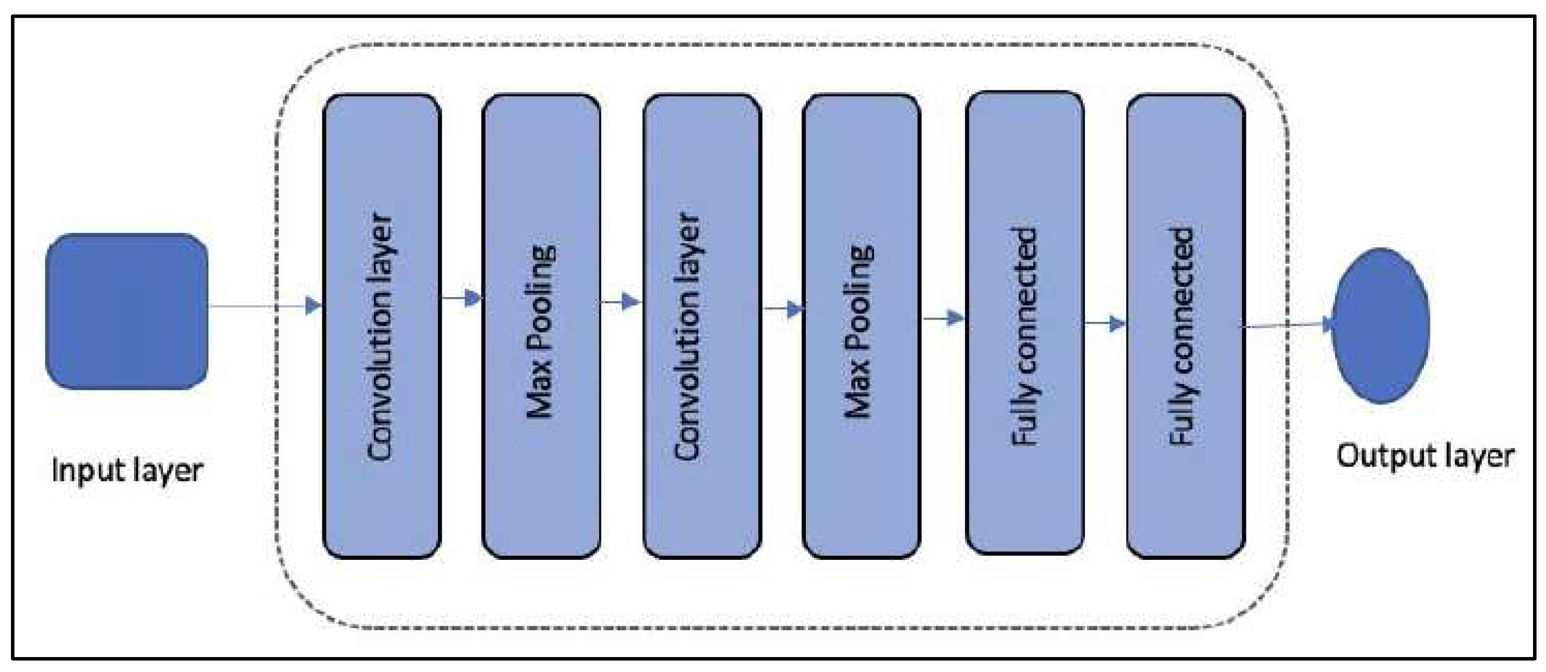
CNNs, or convolutional neural networks, are advanced multi-layer neural networks modeled after biological visual systems. Kunihiko Fukushima’s 1980 neocognitron, which recognized visual patterns hierarchically [59], originally inspired CNNs. LeCun [23] popularized CNNs, revolutionizing image processing by eliminating the need for manual feature extraction. To efficiently handle visual information, they work by processing data directly from matrices or tensors, particularly in color imaging [60]. The basic structure of a CNN can be seen in Figure 3 [60].
In convolutional neural networks, each point in an input image is processed using a convolution operation with a filter, or kernel, which moves across the image by a defined number of pixels known as the “stride”. Small strides can cause overlapping information, while zero padding—adding a border of zeros around the image—helps maintain the output size. Let’s consider a scenario where C0 filters was applied, also referred to as kernels, each with a size of k × k, to an input image. If the dimensions of the input image are Wi × Hi × Ci (where Wi represents the width, Hi the height, and Ci the number of channels, typically Ci = 3 for RGB images), the resulting output volume will have dimensions of W0 × H0 × C0. In this context, C0 corresponds to the number of filters that are employed in the convolution operation where the parameters “P” and “S” are used to denote “padding” and “stride” [59]:
When applying a convolution operation between an image I and a filter Kl, where the image has three channels and the filter is of size 5 × 5 × 3 (where 3 corresponds to the number of channels of the input image), the convolution operation can be expressed mathematically as follows: Let I be the input image with dimensions Wi × Hi × 3, and Kl be the filter with dimensions 5 × 5 × 3. The result of the convolution operation between image I and filter Kl can be expressed as follows [59]:
where (I ∗ Kl) _ {i, j} represents the value at position (i, j) in the output feature map after applying filter Kl to the image I. The triple summation represents the convolution operation, where x and y iterate over the spatial dimensions of the filter (5 × 5), and c iterates over the color channels of the input image (three channels). This formula computes the dot product between the filter Kl and the corresponding region of the input image I for each position (i, j) in the output feature map. If the image has three channels and is linked to filters Kl (l = 1,…, C0) with dimensions 5 × 5 × 3 (where 3 is the number of channels in the input image), then the following equation can be used to describe the convolution between image I and filter Kl [59]:
where z(x) is the output of the convolution operation for the image patch x, is the activation function, often the ReLU function, K is the filter (kernel) being applied, and b is a bias term [59].
ResNet
He et al. explored deeper CNNs and identified the “vanishing gradient” problem as a major challenge, mitigated by normalization and specific initializations but still affecting performance without overfitting. The authors took an innovative approach to this problem. They used a pre-trained shallower model and added identity mapping layers to make the deeper network perform like the shallower one. To solve degradation, they created a deep residual learning framework [61]. In their network architecture, they used residual mapping (expressed as H(x) = F(x) + x) rather than the desired mapping (H(x)). They appropriately named their residual mapping model ResNet [61]. The ResNet architecture consists of stacked blocks with 3 × 3 convolutional layers. To improve network performance, they periodically doubled the number of filters and set layer strides to 2. An illustration of a residual block is shown in Figure 4. The initial network layer is a 7 × 7 convolutional layer. However, the architecture lacks fully connected layers at the end. The ILSVRC-2014 competition tested ResNet with 34, 50, 101, and 152 layers. Like GoogleNet, they added a bottleneck layer to CNNs with depths over 50 to reduce dimensionality and improve efficiency. The bottleneck design included 1 × 1, 3 × 3, and 1 × 1 convolutional layers. The 152-layer ResNet network is eight times deeper than VGG networks, demonstrating its depth and capability [61].
2.4. Long Short-Term Memory (LSTM)
Gated recurrent neural networks (RNNs), particularly LSTM and those based on the gated recurrent unit (GRU), are highly effective for sequential data processing. These networks prevent the extremes of gradient annihilation or explosion, similar to leaky units, by allowing adjustable connection weights across time steps for extended information retention. This flexibility helps in scenarios such as sequence processing, where sub-sequences need isolated consideration without prior state influence. The unique feature of gated RNNs is their ability to learn when to reset this state autonomously, avoiding reliance on preset judgements. The LSTM model, for example, enhances this by incorporating adaptable self-loops that maintain gradient flow over time, making these networks versatile across applications such as language translation, speech recognition, and more [59].
Figure 5 depicts the block diagram of the LSTM. The forward propagation equations for a shallow recurrent network design are provided below. The most important component is the state unit a(t) that has a linear self-loop similar to the leaky units described in the previous section. However, here, the self-loop weight (or the associated time constant) is controlled by a forget gate unit fi(t) (for time step t and cell i) that sets this weight to a value between 0 and 1 via a sigmoid unit [59]:
where x(t) is the current input vector; h(t) is the current hidden layer vector, containing the outputs of all the LSTM cells; and bf, Uf, Wf are respectively biases, input weights, and recurrent weights for the forget gates. The LSTM cell internal state is thus updated as follows, but with a conditional self-loop weight fi(t) [59]:
where b, U, and W denote the biases, input weights, and recurrent weights into the LSTM cell, respectively. The external input gate unit gi(t) is computed similarly to the forget gate (with a sigmoid unit to obtain a gating value between 0 and 1), but with its own parameters [59]:
The output hi(t) of the LSTM cell can also be shut off via the output gate qi(t), which also uses a sigmoid unit for gating [59]:
where parameters bo, Uo, Wo are its biases, input weights, and recurrent weights, respectively. Among the variants, one can choose to use the cell state si(t) as an extra input (with its weight) into the three gates of the i-th unit, as shown in Figure 5. This would require three additional parameters [59].
Figure 5.
Block diagram of the LSTM recurrent network [59].
Figure 5.
Block diagram of the LSTM recurrent network [59].

Transfer Learning—LSTM
Traditional supervised machine learning (ML) trains models on labeled data from a specific task and domain, anticipating their success in similar future scenarios. However, we often need to train new models from scratch when encountering different tasks or domains. Transfer learning addresses this by using knowledge from previously trained models on new but related problems and efficiently applying learned insights across various applications. This approach is crucial in contexts such as computer vision, where data can be scarce and expensive, helping to bridge gaps in data availability [62]. Figure 6 shows a flowchart that explains the work of transfer learning.
3. Proposed LSTM-CNN Model
Deepfake videos are often short and low-resolution, making them suspicious of being synthetic. However, they often display imperfections such as artefacts, resolution variations, and color shifts due to limitations in the deepfake learning algorithm. These flaws are more noticeable when the training dataset lacks comprehensive coverage of different facial angles and lighting conditions, making it difficult to identify and categorize the videos. To find deepfakes, an architecture made up of simple layers has been suggested in this work. The proposed model focuses on advancing the field of deepfake detection through the introduction of a novel approach. The presented research emphasizes the efficacy of leveraging transfer learning within a hybrid architecture, combining CNNs and LSTM networks. Transfer learning facilitates the model’s ability to boil insights from pre-trained networks, enhancing its proficiency in distinguishing deepfake images. The hybrid CNN-LSTM model showcased notable success in combating deep fakes by harnessing the spatial awareness of CNNs and the temporal context understanding of LSTMs. By amalgamating spatial and temporal analysis through the hybrid CNN-LSTM architecture, this study contributes to the growing body of knowledge surrounding deepfake detection, offering a promising solution in the ongoing battle against malicious image manipulation.
In the previous hybrid methods, the dataset underwent analysis and processing via a CNN. The results of the CNN will be processed using LSTM, and, after that, the final results will be obtained. The hybrid method suggested in this paper operates in a distinct manner compared to previous methods, as it incorporates the fusion of CNN and LSTM. The LSTM model is employed subsequent to each layer of the CNN. The process continues according to the number of CNN layers. Three models were used in the proposed method in this paper (model0 (simple), model1 (+dropout), and model2 (+residual blocks)). The transfer learning technique was used in these models; the transfer learning feature captures the “knowledge” that a model “acquired” during training on the initial task and dataset and applies this knowledge to the next model, as explained in the pseudo code in Algorithm 1.
| Algorithm 1: pseudo code for the proposed hybrid method |
Analyze recorded decisions to evaluate the model performance Return deepfake_detected |
In Figure 7, a flowchart of previous hybrid methods can be observed (Figure 7a) and a flowchart of the proposed hybrid method is shown (Figure 7b).
To make the proposed model work better, residual blocks were added. The diagram in Figure 8 illustrates the three proposed blocks. The simple and residual blocks consist of three convolutional layers with ReLU and padding the same activation functions; the symbols n and s represent the number and size of the filters. In the residual block, the output of the first convolution layer is added to the output of the last convolution layer, and a ReLU activation function is applied to the result obtained. The overall architecture of the proposed model is composed of five simple (model0), dropout (model1), or residual (model2) blocks with s = (1, 3, 3, 6, and 9) and n = (16, 32, 32, 64, and 128); after each block, a Max pooling layer is added (except for the first block). Two fully connected layers are added, one with 32 nodes and the last with a single node, followed by the sigmoid function to obtain the classification result (binary classification). Each model has 4.7 million parameters.
3.1. Subsubsection Implementation Tools
To implement and optimize the proposed model, user-friendly open-source DL frameworks that aimed to streamline the development of intricate and large-scale models were accessed. A DL framework serves as an interface, library, or tool designed to facilitate the creation of DL models with ease and speed without the need to delve into the intricate details of underlying algorithms. These frameworks offer a clear and concise means to define models, utilizing a set of pre-configured and optimized components. Some of the most widely used frameworks include the following:
- TensorFlow: Researchers and engineers from the Google Brain team developed TensorFlow, which stands as the most commonly used library in the field of DL. Its popularity is attributed to its support for multiple programming languages, including Python, C++, and R. TensorFlow boasts a flexible architecture that allows the deployment of DL models on single or multiple CPUs, as well as GPUs. It finds applications in various domains, including the following:
- Text-based tasks: language detection, text summarization;
- Image analysis: image captioning, facial recognition, object detection;
- Audio analysis;
- Time-series analysis.
- Keras: Written in Python, Keras can run on CNTK, Theano, and TensorFlow. Keras serves as a high-level API designed to enable rapid experimentation. It supports both CNNs and RNNs and seamlessly operates on both CPUs and GPUs. Keras offers various architectural options, such as those used for image classification, to tackle a wide range of problems efficiently;
- PyTorch: PyTorch is a port of the Torch DL framework and can be employed to construct deep neural networks and perform tensor computations. While Torch is based on Lua, PyTorch runs on Python. It is a Python package that facilitates tensor calculations, wherein tensors are multidimensional arrays similar to numpy’s ndarrays and can be executed on GPUs. PyTorch is versatile and capable of addressing diverse DL challenges, including the following:
- Image tasks (detection, classification, etc.);
- Natural Language Processing (NLP);
- Reinforcement learning.
These DL frameworks have democratized the field of DL, making it more accessible to a broader audience and accelerating progress in the development of advanced DL models.
3.2. Implementation Environment
The proposed model was implemented on the Kaggle platform, which provides a cloud-based environment for data science and machine learning tasks. Kaggle is accessible through www.kaggle.com (accessed on 1 December 2023) and offers both CPU and GPU computation capabilities for running complex machine learning models. Python 3 was used for implementing the model. Python is a widely used programming language in the machine learning community due to its simplicity and the vast availability of libraries and frameworks. It is available at www.python.org (accessed on 1 December 2023). Keras, a high-level neural network API, was used with Tensor Flow serving as the backend computation framework. TensorFlow is an open-source library for numerical computation and machine learning. Keras provides a more user-friendly interface for building and training deep learning models on top of TensorFlow. More information can be found at www.tensorflow.org (accessed on 1 December 2023). The hardware specifications include the following:
- OS: Windows 11 x86_64;
- CPU: Intel (R) CPU @ 2.00 GHz;
- RAM: 16 GB;
- GPU: NVIDIA GeForce GPU;
- GPU Memory: 16 GB.
3.3. Choice of Dataset
Two datasets were used in this study, as they were worked on individually (each data set separately). The data that were worked on are shown below:
- The first dataset used was the Deepfake Detection Challenge (DFDC). This is a key resource for digital media authentication, specifically deepfake detection. A collaboration between Facebook, the Partnership on AI, Microsoft, and academics launched the DFDC. It aims to advance deepfake detection technology to detect realistic-looking AI-generated fake videos. The dataset has many videos. These include many deepfakes and real videos. Deepfake videos were created using various deep learning methods, making the dataset diverse and difficult. One of the largest publicly available datasets, the DFDC contains thousands of videos. This scale is essential for training and testing large-data deep learning models. Researchers and developers train machine-learning models to recognize manipulated videos using this dataset. DFDC videos are diverse and complex, making them ideal for testing advanced detection algorithms. The DFDC wants to stop misinformation and protect digital media by improving deepfake detection. The dataset includes 119,122 224 × 224 images (84% fake, 16% real) [63];
- The second dataset is the Ciplab dataset. Datasets usually contain a large number of images or videos, often annotated or labeled to facilitate supervised learning. The content might include diverse subjects, environments, and conditions to ensure robustness in algorithm training. In the case of generative models such as Generative Adversarial Networks (GANs), generating counterfeit face images is a straightforward task. Consequently, a classifier can be trained by using these synthetically generated images, and these classifiers tend to perform exceptionally well in discriminating between real and GAN-generated face images. It is reasonable to assume that these classifiers learn patterns inherent to images produced using GANs. The dataset contains 23,632 224 × 224 images (fake: 60%, real: 40%) [64].
3.4. Classification Configuration
In binary classification tasks (e.g., real vs. deepfake), check for class imbalance issues. If one class is significantly underrepresented, consider using techniques such as over-sampling or under-sampling to balance the dataset. Data cleaning was performed to address missing values, outliers, and inconsistencies. This step is crucial to ensuring that the overall size of the retained dataset is unified. The following configuration was considered in all stages of training the proposed model:
- Preprocessing dataset: 19,148 real images and 19,148 fake images were used. The whole dataset was divided into two subsets, where 80% represented the training set (subset intended for training the model) and the rest was one evaluation set (subset intended for evaluation). The size of the images was 128 × 128;
- Model learning: since the classification type is binary, the binary-cross entropy 5.4 function was chosen to calculate the error rate for each iteration of training.
For model optimization, the Adam was used to update the network weights during model training. The learning rate with an initial value of 10−4 was divided by 10 if the learning precision did not increase during two successive epochs, up to the minimum value 106.
4. Experimental Results and Discussion
Several experiments with different batch sizes and dropouts (overfitting problem) were performed. Additionally, additional residual blocks were added to the model and the model was compared with and without these blocks. The training and validation precision (accuracy) and error rate (Loss) were used to evaluate the performance of the model:
where
- TP: true positive;
- TN: true negative;
- FP: false positive;
- FN: false negative.
4.1. Epochs, Batch Size, and Iterations
Due to the size of the dataset and the memory constraints of the computer unit utilized for training, it was not possible to take all the training data into an algorithm in a single pass in most cases. Epochs, batch size, and iterations are necessary terms to better understand how data are best divided into smaller pieces.
- The epoch flows when the complete dataset went through the neural network and the weights were adjusted precisely once. It is necessary to partition the dataset into mini-batches if it cannot be fed to the algorithm all at once.
- The batch size represents all of the training samples included in a single mini-batch.
- The iteration indicates the number of network settings updated.
4.2. Batch Size
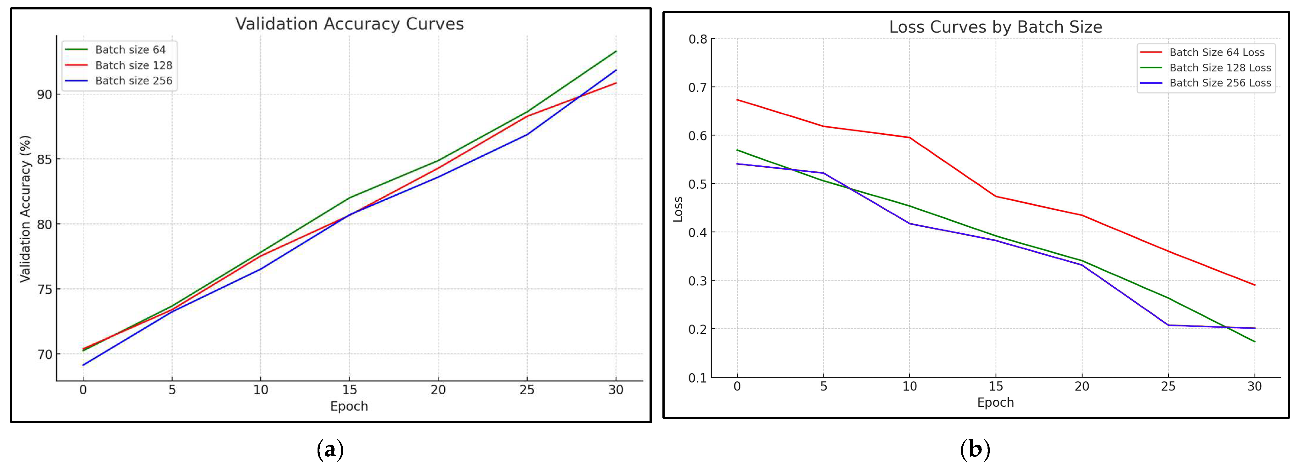
In the proposed case, it was the number of trained images in an iteration before updating the network weights. Figure 9 shows the accuracy and learning error rate achieved with batch sizes of 64, 128, and 256. From Figure 9, it is obviously the batch size with the value 64 that gives the best result. For validation, Figure 10 shows the validation accuracy and validation error rate with different batch sizes of 64, 128, and 256. From Figure 10, it is obvious that the batch size with the best result for validation is 128.
4.3. Dropout
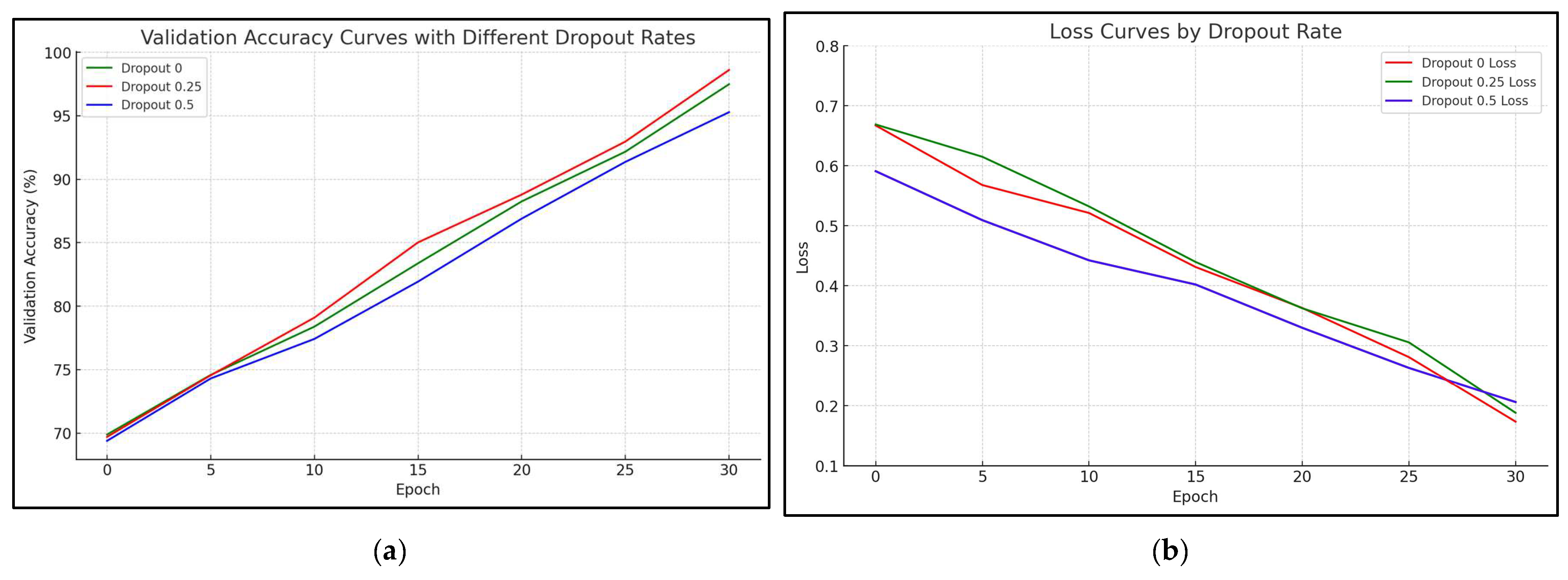
In order to prove the validation results, the dropout regulation technique was used. The key idea was to randomly remove units (with their connections) from the neural network during training. The results in Figure 11 represent the accuracy and error rate during the validation phase with dropout rates of 0, 0.25, and 0.5. It is clear that the use of dropout minimized the error rate and the problem of overfitting. In addition, an improvement in precision was noticed. From Figure 11, it is obvious that the dropout rate with the best result is 0.25.
4.4. Residual Blocks
After using the residual blocks in the model, the obtained results in Figure 12 show that the use of residual blocks improved the model performance in terms of accuracy and reduced the error rate; this effect also appears in the speed of model learning.
4.5. Final Results
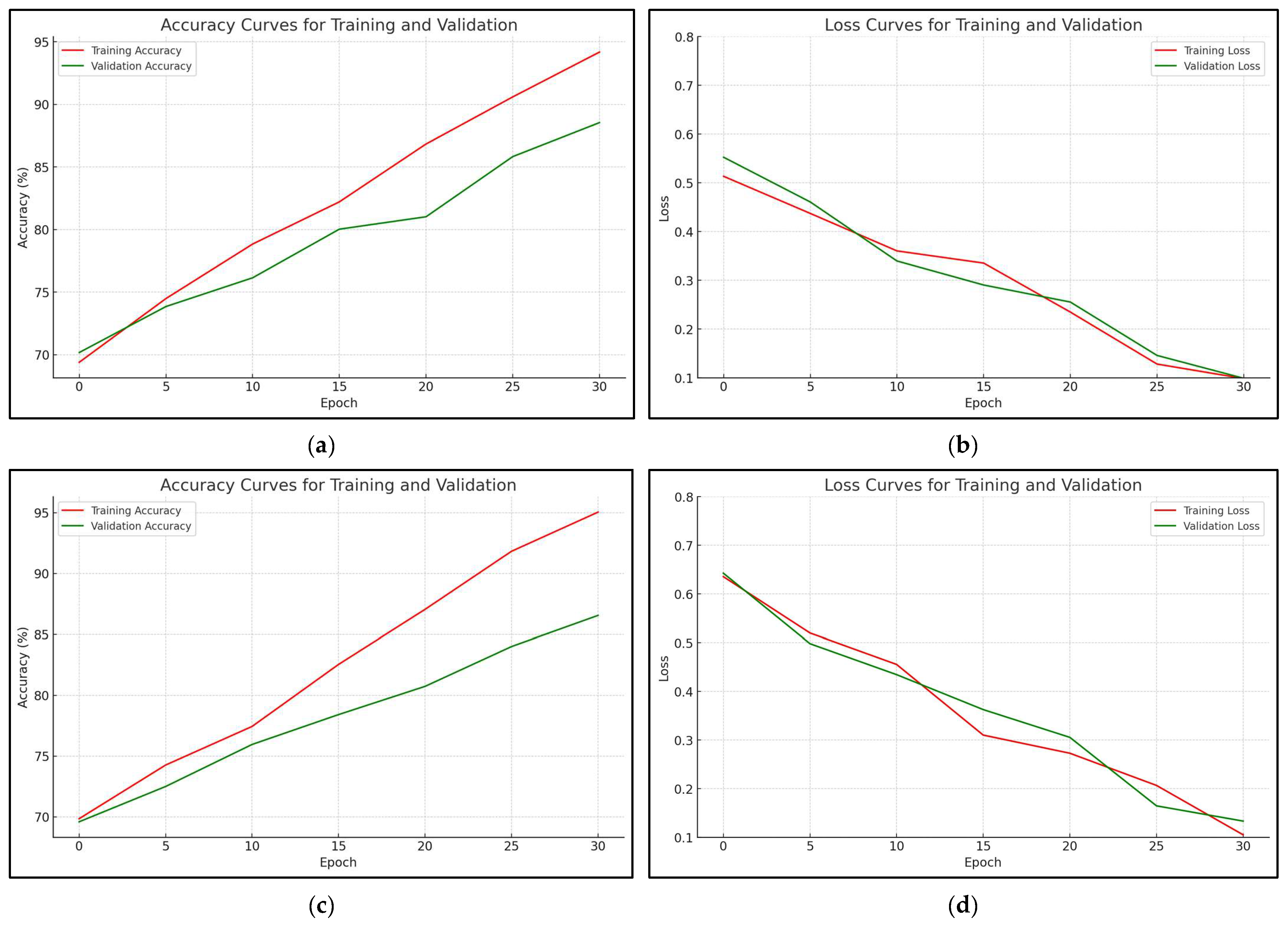
The curves in Figure 13, Figure 14 and Figure 15 represent the precision and error rate of the three models.
Model0 represents the initial model; the results shown in Table 2 were obtained after 15 epochs.
In Model1, the dropout regularization technique was used.
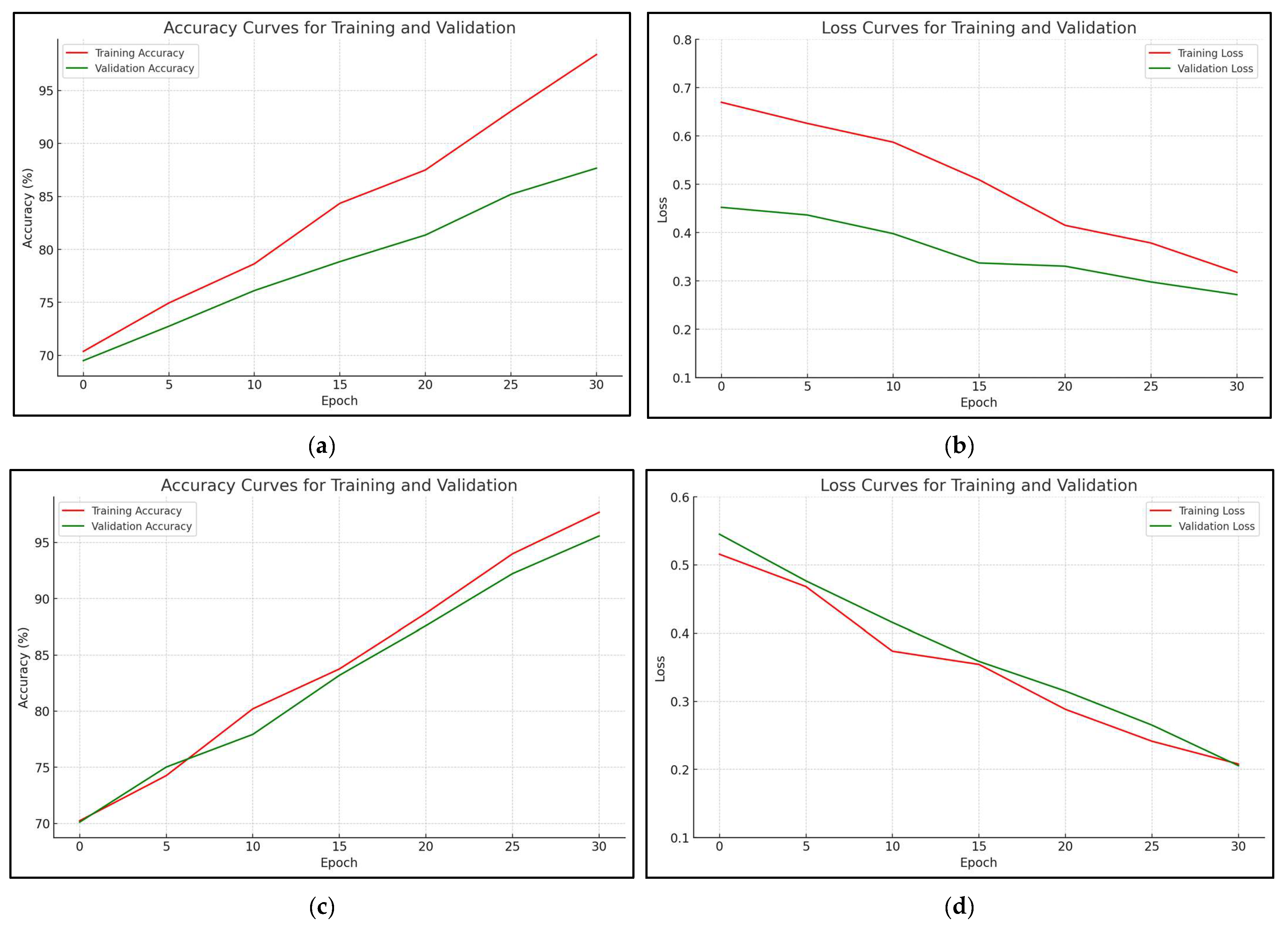
Figure 14.
Model 1: training and validation results (accuracy and error rate) for both datasets: (a) Model1 accuracy for the DFDC dataset, (b) Model1 error rate for the DFDC dataset, (c) Model1 accuracy for the Ciplab dataset, (d) Model1 error rate for the Ciplab dataset.
Figure 14.
Model 1: training and validation results (accuracy and error rate) for both datasets: (a) Model1 accuracy for the DFDC dataset, (b) Model1 error rate for the DFDC dataset, (c) Model1 accuracy for the Ciplab dataset, (d) Model1 error rate for the Ciplab dataset.

The best result of model1 is shown in Table 3.
Finally, model2 had an architecture with the residual blocks.
Figure 15.
Model2: training and validation results (accuracy and error rate) for both datasets: (a) Model2 accuracy for the DFDC dataset, (b) Model2 error rate for the DFDC dataset, (c) Model2 accuracy for the Ciplab dataset, (d) Model2 error rate for the Ciplab dataset.
Figure 15.
Model2: training and validation results (accuracy and error rate) for both datasets: (a) Model2 accuracy for the DFDC dataset, (b) Model2 error rate for the DFDC dataset, (c) Model2 accuracy for the Ciplab dataset, (d) Model2 error rate for the Ciplab dataset.

The obtained accuracy and error rate of Model2 are shown in Table 4.
Section 4.5 discusses the final results of the three proposed models in this study, as depicted in Figure 13, Figure 14 and Figure 15. It is obvious that Model2 outperforms the other two models in terms of accuracy. Table 2, Table 3 and Table 4 present the accuracy and error rate of the three models when applied to the DFDC and Ciplab datasets. Figure 16 presents a comparison of the precision between the proposed models and other related works in Section 1.3. It is evident that Model2 gives better results than the other related works in Section 1.3. Table 5 presents a comparison of the error rate and accuracy between the proposed Model2 and other related works in Section 1.3. It is clear that Model2 yields superior results than the other related works. Figure 17 and Figure 18 provide an explanation of the precision and recall of the proposed Model2, respectively.
5. Conclusions
In this paper, a novel DL architecture model for deepfake detection was proposed using a hybrid combination of LSTM and CNN methods and implemented using the Python language and Kaggle platform. Two datasets of DFDC and Ciplab were selected to evaluate the performance of the proposed model. The preprocessing of the dataset included using 19,148 real images and 19,148 fake images. The whole dataset was divided into two subsets, where 80% represented the training set with an image size of 128 × 128. Additionally, the binary-cross entropy 5.4 function was utilized to calculate the error rate for each iteration of training. The results obtained indicated an accuracy of 97.32% and 98.24% and a low error rate of 0.15% and 0.26% for the two datasets used, respectively. This confirmed the adaptability of the proposed model in handling accurate deepfake prediction because LSTMs can capture sequential temporal dependencies effectively. LSTMs can describe temporal connections between frames to uncover deepfake discrepancies. Meanwhile, using CNN it is possible to evaluate the frame’s content to find visual artefacts, inconsistencies, or strange patterns that may indicate manipulation or synthesis. Therefore, combining LSTM and CNN provides the ability to concentrate on the areas in which it excels, which could result in a model that is both more efficient and effective. Moreover, it allows the model to adapt to a wide range of deepfake generation techniques.
Author Contributions
Methodology, O.A.H.H.A.-D.; software, O.A.H.H.A.-D.; validation, O.A.H.H.A.-D.; formal analysis, O.A.H.H.A.-D.; investigation, O.A.H.H.A.-D.; writing—original draft preparation, O.A.H.H.A.-D.; writing—review and editing, S.K.; supervision, S.K.; project administration, S.K. All authors have read and agreed to the published version of the manuscript.
Funding
This research received no external funding.
Data Availability Statement
Data are contained within the article.
Conflicts of Interest
The authors declare no conflicts of interest.
References
- Gordon, G. The Internet a Philosophical Inquiry; Routledge: London, UK; New York, NY, USA, 1999; 190p, ISBN 9780415197496. [Google Scholar]
- Maras, M.-H.; Alexandrou, A. Determining authenticity of video evidence in the age of artificial intelligence and in the wake of Deepfake videos. Int. J. Evid. Proof 2019, 23, 255–262. [Google Scholar] [CrossRef]
- Dolhansky, B.; Bitton, J.; Pflaum, B.; Lu, J.; Howes, R.; Wang, M.; Ferrer, C. The deepfake detection challenge dataset. arXiv 2020, arXiv:2006.07397. [Google Scholar]
- Hasan, H.R.; Salah, K. Combating Deepfake Videos Using Blockchain and Smart Contracts. IEEE Access 2019, 7, 41596–41606. [Google Scholar] [CrossRef]
- De keersmaecker, J.; Roets, A. ‘Fake news’: Incorrect, but hard to correct. The role of cognitive ability on the impact of false information on social impressions. Intelligence 2017, 65, 107–110. [Google Scholar] [CrossRef]
- Anderson, K.E. Getting acquainted with social networks and apps: Social Media in 2017. Libr. Hi Tech News 2017, 34, 1–6. [Google Scholar] [CrossRef]
- Available online: https://edition.cnn.com/2019/06/11/tech/zuckerberg-deepfake/index.html (accessed on 7 June 2019).
- Barsha, L.; Keshav, T.; Sung-Hyun, Y. Detection of Image Level Forgery with Various Constraints Using DFDC Full and Sample Datasets. Sensors 2022, 22, 9121. [Google Scholar] [CrossRef] [PubMed]
- Zao Download Android, iPhone, iPad 2020. Available online: https://zaodownload.com/ (accessed on 12 December 2023).
- Laan Labs. Available online: http://faceswaplive.com/ (accessed on 4 January 2023).
- DeepfakesWeb.com. Available online: https://deepfakesweb.com/ (accessed on 4 January 2023).
- Anthropics Technology Ltd. Available online: https://www.anthropics.com/portraitpro/ (accessed on 4 January 2023).
- Neocortext. Available online: https://hey.reface.ai/ (accessed on 4 January 2023).
- The Audacity Team. Available online: https://voice.ai/hub/app/free-voice-changer-for-audacity/ (accessed on 21 September 2022).
- Magix Software GmbH. Available online: https://www.magix.com/us/music-editing/sound-forge/ (accessed on 4 January 2023).
- Adobe. Available online: https://www.photoshop.com/en (accessed on 4 January 2023).
- Available online: https://apps.apple.com/us/app/agingbooth/id357467791 (accessed on 13 June 2023).
- Roettgers, J. How AI Tech Is Changing Dubbing, Making Stars Like David Beckham Multilingual. 2019. Available online: https://variety.com/2019/biz/news/ai-dubbing-david-beckham-multilingual-1203309213/ (accessed on 4 January 2023).
- Lee, D. Deepfake Salvador Dali Takes Selfies with Museum Visitors, The Verge. 2019. Available online: https://www.theverge. com/2019/5/10/18540953/salvador-dali-lives-deepfake-museum (accessed on 4 January 2023).
- Güera, D.; Delp, E.J. Deepfake Video Detection Using Recurrent Neural Networks. In Proceedings of the 15th IEEE International Conference on Advanced Video and Signal Based Surveillance (AVSS), Auckland, New Zealand, 27–30 November 2018; pp. 1–6. [Google Scholar]
- Diakopoulos, N.; Johnson, D. Anticipating and addressing the ethical implications of deepfakes in the context of elections. New Media Soc. 2021, 23, 2072–2098. [Google Scholar] [CrossRef]
- Pantserev, K. The malicious use of AI-based deepfake technology as the new threat to psychological security and political stability. In Cyber Defence in the Age of AI, Smart Societies and Augmented Humanity; Springer: Cham, Switzerland, 2020; pp. 37–55. [Google Scholar]
- Oliveira, L. The current state of fake news. Procedia Comput. Sci. 2017, 121, 817–825. [Google Scholar]
- Zhou, X.; Zafarani, R. A survey of fake news: Fundamental theories, detection methods, and opportunities. ACM Comput. Surv. (CSUR) 2020, 53, 1–40. [Google Scholar] [CrossRef]
- Kietzmann, J.; Lee, L.; McCarthy, I.; Kietzmann, T. Deepfakes: Trick or treat? Bus. Horiz. 2020, 63, 135–146. [Google Scholar] [CrossRef]
- Zakharov, E.; Shysheya, A.; Burkov, E.; Lempitsky, V. Few-Shot Adversarial Learning of Realistic Neural Talking Head Models. In Proceedings of the IEEE/CVF International Conference on Computer Vision (ICCV), Seoul, Republic of Korea, 27 October–2 November 2019; pp. 9458–9467. [Google Scholar]
- Damiani, J. A Voice Deepfake Was Used to Scam a CEO Out of $243,000. 2019. Available online: https://www.forbes.com/sites/ jessedamiani/2019/09/03/a-voice-deepfake-was-used-to-scam-a-ceo-out-of-243000/?sh=173f55a52241 (accessed on 4 January 2023).
- Korshunov, P.; Marcel, S. Vulnerability assessment and detection of Deepfake videos. In Proceedings of the International Conference on Biometrics (ICB), Crete, Greece, 4–7 June 2019; pp. 1–6. [Google Scholar]
- Scherhag, U.; Nautsch, A.; Rathgeb, C.; Gomez-Barrero, M.; Veldhuis, R.N.; Spreeuwers, L.; Schils, M.; Maltoni, D.; Grother, P.; Marcel, S.; et al. Biometric Systems under Morphing Attacks: Assessment of Morphing Techniques and Vulnerability Reporting. In Proceedings of the International Conference of the Biometrics Special Interest Group, Darmstadt, Germany, 20–22 September 2017; pp. 1–7. [Google Scholar]
- Rathgeb, C.; Drozdowski, P.; Busch, C. Detection of Makeup Presentation Attacks based on Deep Face Representations. In Proceedings of the 25th International Conference on Pattern Recognition (ICPR), Virtual Event, 10–15 January 2021; pp. 3443–3450. [Google Scholar]
- Majumdar, P.; Agarwal, A.; Singh, R.; Vatsa, M. Evading Face Recognition via Partial Tampering of Faces. In Proceedings of the IEEE/CVF Conference on Computer Vision and Pattern Recognition Workshops, Long Beach, CA, USA, 16–17 June 2019; pp. 11–20. [Google Scholar]
- Ferrara, M.; Franco, A.; Maltoni, D.; Sun, Y. On the impact of alterations on face photo recognition accuracy. In Proceedings of the International Conference on Image Analysis and Processing, Naples, Italy, 9–13 September 2013; pp. 743–751. [Google Scholar]
- Yang, L.; Song, Q.; Wu, Y. Attacks on state-of-the-art face recognition using attentional adversarial attack generative network. Multimed. Tools Appl. 2021, 80, 855–875. [Google Scholar]
- Colbois, L.; Pereira, T.; Marcel, S. On the use of automatically generated synthetic image datasets for benchmarking face recognition. arXiv 2021, arXiv:2106.04215. [Google Scholar]
- Huang, C.-Y.; Lin, Y.Y.; Lee, H.-Y.; Lee, L.-S. Defending Your Voice: Adversarial Attack on Voice Conversion. In Proceedings of the IEEE Spoken Language Technology Workshop (SLT), Virtual, 19–22 January 2021; pp. 552–559. [Google Scholar]
- Kong, C.; Chen, B.; Li, H.; Wang, S.; Rocha, A.; Kwong, S. Detect and Locate: Exposing Face Manipulation by Semantic- and Noise-Level Telltales. IEEE Trans. Inf. Forensics Secur. 2022, 17, 1741–1756. [Google Scholar] [CrossRef]
- Miao, C.; Chu, Q.; Tan, Z.; Jin, Z.; Zhuang, W.; Wu, Y.; Liu, B.; Hu, H.; Yu, N. Multi-spectral Class Center Network for Face Manipulation Detection and Localization. IEEE Trans. Multimed. 2022, 24, 377–385. [Google Scholar]
- Luo, A.; Kong, C.; Huang, J.; Hu, Y.; Kang, X.; Kot, A.C. Beyond the Prior Forgery Knowledge: Mining Critical Clues for General Face Forgery Detection. IEEE Trans. Inf. Forensics Secur. 2024, 19, 1168–1182. [Google Scholar] [CrossRef]
- Sun, K.; Yao, T.; Chen, S.; Ding, S.; Li, J.; Ji, R. Dual Contrastive Learning for General Face Forgery Detection. Proc. AAAI Conf. Artif. Intell. 2022, 36, 2316–2324. [Google Scholar] [CrossRef]
- Li, L.; Bao, J.; Zhang, T.; Yang, H.; Chen, D.; Wen, F.; Guo, B. Face X-Ray for More General Face Forgery Detection. In Proceedings of the 2020 IEEE/CVF Conference on Computer Vision and Pattern Recognition (CVPR), Seattle, WA, USA, 13–19 June 2020; pp. 5000–5009. [Google Scholar]
- Qian, Y.; Yin, G.; Sheng, L.; Chen, Z.; Shao, J. Thinking in Frequency: Face Forgery Detection by Mining Frequency-Aware Clues. In Computer Vision–ECCV 2020; Lecture Notes in Computer Science; Vedaldi, A., Bischof, H., Brox, T., Frahm, J.M., Eds.; Springer: Berlin/Heidelberg, Germany, 2020; p. 12357. [Google Scholar]
- Taha, M.Q.; Kurnaz, S. Droop Control Optimization for Improved Power Sharing in AC Islanded Microgrids Based on Centripetal Force Gravity Search Algorithm. Energies 2023, 16, 7953. [Google Scholar] [CrossRef]
- Al-dulaimi, F.N.S.; Kurnaz, S. Optimized Distributed Cooperative Control for Islanded Microgrid Based on Dragonfly Algorithm. Energies 2023, 16, 7675. [Google Scholar] [CrossRef]
- Hussain, S.; Neekhara, P.; Jere, M.; Koushanfar, F.; McAuley, J. Adversarial deepfakes: Evaluating vulnerability of deepfake detectors to adversarial examples. In Proceedings of the IEEE/CVF Winter Conference on Applications of Computer Vision, Virtual, 5–9 January 2021; pp. 3348–3357. [Google Scholar]
- Mehta, V.; Gupta, P.; Subramanian, R.; Dhall, A. FakeBuster: A DeepFakes detection tool for video conferencing scenarios. In Proceedings of the International Conference on Intelligent User Interfaces-Companion, College Station, TX, USA, 13–17 April 2021; pp. 61–63. [Google Scholar]
- Xu, J.-F.; Wang, R.; Huang, Y.; Guo, Q.; Ma, L.; Liu, Y. Countering Malicious DeepFakes: Survey, Battleground, and Horizon. Int. J. Comput. Vis. 2022, 130, 1678–1734. [Google Scholar]
- Amerini, I.; Galteri, L.; Caldelli, R.; Del Bimbo, A. Deepfake video detection through optical flow based CNN. In Proceedings of the IEEE/CVF International Conference on Computer Vision Workshops, Seoul, Republic of Korea, 27–28 October 2019. [Google Scholar]
- Aneja, S.; Nießner, M. Generalized zero and few-shot transfer for facial forgery detection. arXiv 2020, arXiv:2006.11863. [Google Scholar]
- de Lima, O.; Franklin, S.; Basu, S.; Karwoski, B.; George, A. Deepfake Detection using Spatiotemporal Convolutional Networks. arXiv 2020, arXiv:2006.14749v1. [Google Scholar]
- Dogonadze, N.; Obernosterer, J.; Hou, J. Deep Face Forgery Detection. arXiv 2020, arXiv:2004.11804. [Google Scholar]
- Khan, S.A.; Artusi, A.; Dai, H. Adversarially robust deepfake media detection using fused convolutional neural network predictions. arXiv 2021, arXiv:2102.05950. [Google Scholar]
- Shad, H.S.; Rizvee, M.M.; Roza, N.T.; Hoq, S.M.A.; Khan, M.M.; Singh, A.; Zaguia, A.; Bourouis, S. Comparative analysis of deepfake image detection method using convolutional neural network. Comput. Intell. Neurosci. 2021, 2021, 3111676. [Google Scholar] [CrossRef] [PubMed]
- Saikia, P.; Dholaria, D.; Yadav, P.; Patel, V.; Roy, M. A hybrid CNN-LSTM model for video deepfake detection by leveraging optical flow features. In Proceedings of the 2022 International Joint Conference on Neural Networks (IJCNN), Padua, Italy, 18–23 July 2022; IEEE: New York, NY, USA, 2022; pp. 1–7. [Google Scholar]
- Mohammad, M. Understanding of Machine Learning with Deep Learning: Architectures, Workflow, Applications and Future Directions. Computers 2023, 12, 91. [Google Scholar] [CrossRef]
- Ali, R.; Kashif, M.; Mubarak, A. A Novel Deep Learning Approach for Deepfake Image Detection. Appl. Sci. 2022, 12, 9820. [Google Scholar] [CrossRef]
- Mirsky, Y.; Lee, W. The creation and detection of deepfakes: A survey. ACM Comput. Surv. 2021, 54, 1–41. [Google Scholar] [CrossRef]
- Andreas, R.; Davide, C.; Luisa, V.; Christian, R.; Justus, T.; Matthias, N. FaceForensics++: Learning to Detect Manipulated Facial Images. arXiv 2019, arXiv:1901.08971v3. [Google Scholar]
- Collins, E.; Bala, R.; Price, B.; Susstrunk, S. Editing in style: Uncovering the local semantics of GANs. In Proceedings of the IEEE/CVF Conference on Computer Vision and Pattern Recognition, Seattle, WA, USA, 13–19 June 2020; pp. 5771–5780. [Google Scholar]
- Goodfellow, I.; Bengio, Y.; Courville, A. Deep Learning; MIT Press: Cambridge, MA, USA, 2016; 800p, ISBN 0262035618, 9780262035613. [Google Scholar]
- Zainab, A.; Rabeah, A.; Jalal, A.; Qazi, E.U.; Kashif, S.; Muhammad, H.F. A Deep Learning-Based Phishing Detection System Using CNN, LSTM, and LSTM-CNN. Electronics 2023, 12, 232. [Google Scholar] [CrossRef]
- He, K.; Zhang, X.; Ren, S.; Sun, J. Deep residual learning for image recognition. In Proceedings of the IEEE Conference on Computer Vision and Pattern Recognition, Las Vegas, NV, USA, 27–30 June 2016; pp. 770–778. [Google Scholar]
- Noel, A.; Shreyanka, K.; Kumar, K.G.S.; Bm, S.; Akshar, B. Autonomous Ship Navigation Methods: A Review. In Proceedings of the International Conference on Marine Engineering and Technology Oman, Muscat, Oman, 5–7 November 2019. [Google Scholar] [CrossRef]
- Available online: https://www.kaggle.com/competitions/deepfake-detection-challenge/data (accessed on 10 April 2023).
- Available online: https://www.kaggle.com/datasets/ciplab/real-and-fake-face-detection (accessed on 10 April 2023).
Figure 1.
Deepfake published on the Instagram social network in July 2019 of Mark Zuckerberg [7].
Figure 1.
Deepfake published on the Instagram social network in July 2019 of Mark Zuckerberg [7].

Figure 2.
Examples of reenactment, replacement, editing, and synthesis deepfakes of the human face [56].
Figure 2.
Examples of reenactment, replacement, editing, and synthesis deepfakes of the human face [56].

Figure 3.
CNN basic architecture [60].
Figure 3.
CNN basic architecture [60].

Figure 4.
Residual learning: a building block [61].
Figure 4.
Residual learning: a building block [61].

Figure 6.
A flowchart showing working of transfer learning [62].
Figure 6.
A flowchart showing working of transfer learning [62].

Figure 7.
Flowchart explaining how the previous hybrid and proposed hybrid method works (comparator): (a) flowchart of previous hybrid methods, (b) flowchart of the proposed method.
Figure 7.
Flowchart explaining how the previous hybrid and proposed hybrid method works (comparator): (a) flowchart of previous hybrid methods, (b) flowchart of the proposed method.

Figure 8.
Blocks proposed in this paper: (a) simple block, (b) dropout block, (c) residual block.

Figure 9.
The accuracy (precision) and learning error rate with different batch sizes: (a) accuracy with batch size of 64, 128, and 256; (b) learning error rate with batch size of 64, 128, and 256.
Figure 9.
The accuracy (precision) and learning error rate with different batch sizes: (a) accuracy with batch size of 64, 128, and 256; (b) learning error rate with batch size of 64, 128, and 256.

Figure 10.
The validation accuracy and validation error rate with different batch sizes: (a) validation accuracy with batch size of 64, 128, and 256; (b) validation error rate with batch size of 64, 128, and 256.
Figure 10.
The validation accuracy and validation error rate with different batch sizes: (a) validation accuracy with batch size of 64, 128, and 256; (b) validation error rate with batch size of 64, 128, and 256.

Figure 11.
Validation accuracy and validation error rate with different dropout rates: (a) validation accuracy with dropout rates of 0, 0.25, and 0.5; (b) validation error rate with dropout rates of 0, 0.25, and 0.5.
Figure 11.
Validation accuracy and validation error rate with different dropout rates: (a) validation accuracy with dropout rates of 0, 0.25, and 0.5; (b) validation error rate with dropout rates of 0, 0.25, and 0.5.

Figure 12.
Validation results: model0 (simple), model1 (+dropout), and model2 (+residual blocks): (a) validation accuracy for the three models and (b) validation error rate for the three models.
Figure 12.
Validation results: model0 (simple), model1 (+dropout), and model2 (+residual blocks): (a) validation accuracy for the three models and (b) validation error rate for the three models.

Figure 13.
Model0: training and validation results (accuracy and error rate) for both datasets: (a) Model0 accuracy for the DFDC dataset, (b) Model0 error rate for the DFDC dataset, (c) Model0 accuracy for the Ciplab dataset, (d) Model0 error rate for the Ciplab dataset.
Figure 13.
Model0: training and validation results (accuracy and error rate) for both datasets: (a) Model0 accuracy for the DFDC dataset, (b) Model0 error rate for the DFDC dataset, (c) Model0 accuracy for the Ciplab dataset, (d) Model0 error rate for the Ciplab dataset.

Figure 16.
Comparison of the precision between the proposed CNN-LSTM model (Model2) with other related works in Section 1.3 [47,48,49,50,51,52,53].

Figure 17.
Precision of the proposed CNN-LSTM (Model2).

Figure 18.
Recall of the proposed CNN-LSTM (Model2).


Table 1.
Comparative analyses of the related works.
| Study | Approach and Model | Dataset | Accuracy |
|---|---|---|---|
| [47] | Optical flow fields based on VGG16 | FaceForensics++ dataset |
|
| [48] | CNN-LSTM using Xception Net | DFDC dataset |
|
| [49] | 3D input data with R3D | Celeb-DF dataset |
|
| [50] | Transfer learning from face recognition and temporal information | FaceForensics++ dataset |
|
| [51] | Fusion of VGG16, InceptionV3, and Xception Net | DFDC dataset |
|
| [52] | Eight different CNN architectures (VGGFace, DenseNet169, DenseNet201, VGG19, VGG16, ResNet50, DenseNet121, and custom models) | Large dataset |
|
| [53] | Hybrid DL of CNN and LSTM with optical flow feature | DFDC, FaceForensics ++, Celeb-DF datasets |
|
| Proposed | Hybrid CNN-LSTM Model Based on Transfer Learning | DFDC, Ciplab datasets |
|
Table 2.
Model0 precision and error rate.
| Dataset | Precision | Error Rate |
|---|---|---|
| DFDC | 94.13% | 05.87% |
| Ciplab | 92.91% | 07.09% |
Table 3.
Model1 precision and error rate.
| Dataset | Precision | Error Rate |
|---|---|---|
| DFDC | 95.32% | 04.68% |
| Ciplab | 95.24% | 04.76% |
Table 4.
Model2 precision and error rate.
| Dataset | Precision | Error Rate |
|---|---|---|
| DFDC | 98.24% | 0.26% |
| Ciplab | 97.32% | 0.15% |
Table 5.
Error rate and accuracy of the proposed CNN-LSTM model (Model2) with other related works in Section 1.3.
Table 5.
Error rate and accuracy of the proposed CNN-LSTM model (Model2) with other related works in Section 1.3.
| Study | Accuracy | Error Rate |
|---|---|---|
| Amerini et al., 2019 [47] | 81.61% | 29.43% |
| Aneja et al., 2020 [48] | 73.20% | 26.8% |
| de Lima et al., 2020 [49] | 97.26% | 02.74% |
| Dogonadze, N et al., 2020 [50] | 77.7 | 22.3% |
| Khan et al., 2021 [51] | 97% | 3% |
| Shad et al., 2021 [52] | 97% | 3% |
| Saikia et al., 2022 [53] | 91.21% | 8.79% |
| Proposed (Model2) | 98.24% | 0.26% |
Disclaimer/Publisher’s Note: The statements, opinions and data contained in all publications are solely those of the individual author(s) and contributor(s) and not of MDPI and/or the editor(s). MDPI and/or the editor(s) disclaim responsibility for any injury to people or property resulting from any ideas, methods, instructions or products referred to in the content. |
© 2024 by the authors. Licensee MDPI, Basel, Switzerland. This article is an open access article distributed under the terms and conditions of the Creative Commons Attribution (CC BY) license (https://creativecommons.org/licenses/by/4.0/).
Share and Cite
MDPI and ACS Style
Al-Dulaimi, O.A.H.H.; Kurnaz, S. A Hybrid CNN-LSTM Approach for Precision Deepfake Image Detection Based on Transfer Learning. Electronics 2024, 13, 1662. https://0-doi-org.brum.beds.ac.uk/10.3390/electronics13091662
AMA Style
Al-Dulaimi OAHH, Kurnaz S. A Hybrid CNN-LSTM Approach for Precision Deepfake Image Detection Based on Transfer Learning. Electronics. 2024; 13(9):1662. https://0-doi-org.brum.beds.ac.uk/10.3390/electronics13091662
Chicago/Turabian StyleAl-Dulaimi, Omar Alfarouk Hadi Hasan, and Sefer Kurnaz. 2024. "A Hybrid CNN-LSTM Approach for Precision Deepfake Image Detection Based on Transfer Learning" Electronics 13, no. 9: 1662. https://0-doi-org.brum.beds.ac.uk/10.3390/electronics13091662
Note that from the first issue of 2016, this journal uses article numbers instead of page numbers. See further details here.