Edge-Enhanced Dual-Stream Perception Network for Monocular Depth Estimation

Abstract

Estimating depth from a single RGB image has a wide range of applications, such as in robot navigation and autonomous driving. Currently, Convolutional Neural Networks based on encoder–decoder architecture are the most popular methods to estimate depth maps. However, convolutional operators have limitations in modeling large-scale dependence, often leading to inaccurate depth predictions at object edges. To address these issues, a new edge-enhanced dual-stream monocular depth estimation method is introduced in this paper. ResNet and Swin Transformer are combined to better extract global and local features, which benefits the estimation of the depth map. To better integrate the information from the two branches of the encoder and the shallow branch of the decoder, we designed a lightweight decoder based on the multi-head Cross-Attention Module. Furthermore, in order to improve the boundary clarity of objects in the depth map, a loss function with an additional penalty for depth estimation error on the edges of objects is presented. The results on three datasets, NYU Depth V2, KITTI, and SUN RGB-D, show that the method presented in this paper achieves better performance for monocular depth estimation. Additionally, it has good generalization capabilities for various scenarios and real-world images.

1. Introduction

Depth estimation is a significant aspect of 3D stereovision, which plays a fundamental role in comprehending the geometric characteristics of the scene and establishing the three-dimensional relationships among objects and their surroundings. This technology assumes a significant role across a spectrum of applications. For instance, in robot navigation, it provides support for self-localization, collision prevention, and path planning efforts. In 3D reconstruction, it helps in clarifying the orientation, posture, and geometric details of objects. In autonomous driving, it enhances the detection of nearby vehicles and pedestrians, making it a vital component in generating detailed, high-resolution maps. Depth information also boosts the accuracy and efficiency of 3D image modeling in augmented reality, which has extensive utilization in production and life.

Methods for acquiring depth information can be divided into two main categories. The first category comprises active depth sensing technologies such as laser radar, millimeter-wave radar, structured light [1], and ToF (Time-of-Flight) [2]. Laser radar has centimeter-level accuracy in depth measurements but is expensive and less effective under adverse weather conditions. Millimeter-wave radar, on the other hand, is more affordable and weather-resistant but offers lower precision and faces significant interference from similar devices [3]. Structured light scanning achieves millimeter-level accuracy but is limited in its suitability for short distances, sensitivity to ambient light, and object movement. In contrast, ToF is cost-effective and easy to use, but produces lower-resolution depth maps and results in high power consumption [4].

The second category includes passive depth estimation techniques such as binocular [5] and multi-ocular [6] stereo matching, along with monocular depth estimation. Methods of binocular and multi-ocular stereo matching calculate depth through disparity maps, demanding extensive computational power and memory, as well as intricate procedures like camera calibration. These methods face challenges in scenes with inconsistent lighting and faint texture features, often resulting in inaccurate depth values and noise. Conversely, monocular depth estimation operates differently by not requiring image rectification or sophisticated equipment. It uses deep neural networks to determine the depth of every pixel in an RGB image taken by a single camera.

Passive methods are often simpler and less expensive to use compared to active methods. Monocular image depth estimation is especially promising for development and application, due to its low hardware cost and adaptability to various environments. Passive algorithms are typically divided into three types: supervised, unsupervised, and semi-supervised methods. Supervised methods require a large volume of precisely annotated Ground Truth data for network training, which usually results in higher depth estimation accuracy. Although unsupervised and semi-supervised methods reduce dependency on data, their depth estimation accuracy generally falls short of supervised methods. Currently, estimation accuracy remains the primary consideration in applications such as autonomous driving and robotic navigation.

In recent years, deep learning has been applied to monocular depth prediction, with Convolutional Neural Networks being the most commonly used method for predicting depth maps [7]. However, convolutional operators have a limited global receptive field, which makes it difficult for them to model long-range dependencies. This can adversely affect the extraction of context information that is crucial for depth estimation tasks. To address this issue, traditional convolutional encoders use consecutively stacked convolutional and downsampling layers to gradually increase the receptive field and enhance the global modeling capabilities of the encoder. However, this approach has the drawback of losing important local information that is closely related to depth estimation tasks, due to the reduction in spatial resolution from downsampling operations. In addition, existing models often produce inaccurate edges of objects in the estimated depth map. In the case that there is a boundary in the image but no depth difference (such as the pattern on a flat carpet), many algorithms often give wrong depth estimates of the pattern.

Studying edge details for depth estimation is a crucial issue for enhancing the accuracy of depth estimation. Accurately estimating edges has long been an unresolved challenge. Most existing monocular estimation methods cannot accurately perceive the edges of objects in images, and the blurriness of edges leads to difficulties in distinguishing closely situated objects in 2D, which becomes a critical problem for tasks that require precise differentiation of similar objects. Edge areas often experience the greatest depth variation within an image, making them vital for the accuracy of depth estimation. In recent years, many researchers have begun to use deep learning technologies to improve the accuracy of depth estimation at edges. Introducing attention mechanisms and multi-scale feature fusion are important strategies to enhance the accuracy of object edges in generated depth maps. Attention mechanisms highlight key parts of the image and allow neural networks to focus more on important features to improve the overall accuracy of the depth estimation. Multi-scale feature fusion, by integrating features of different scales, can more comprehensively capture the rough location and specific details of edges by using a wide range of contextual information and local details to enhance the predictive performance of depth in edge regions. However, although attention mechanisms can increase the model’s sensitivity to key features, they may still struggle to accurately capture all relevant depth information in scenes with complex backgrounds and subtle edges. For example, Li discussed the challenges of using attention mechanisms in monocular depth estimation in his review [8]. Additionally, while multi-scale feature fusion can improve the recognition of edges and details by combining features of different scales, it may face difficulties in handling small-scale or distant objects, as these features may not be prominent or may be lost at lower scales. Furthermore, this fusion strategy increases the complexity of the network, which could lead to overfitting. Therefore, exploring a simple and effective monocular depth estimation loss function to reinforce edge information is highly necessary.

We propose a new monocular depth estimation using an edge-enhanced dual-stream deep neural network. This method uses the attention mechanism to model the relationships among all pixels in the input image, which helps extract global and local detail information. We also introduce a new loss to guide the network training to better estimate depth maps at edges, reduce misjudgments, and enhance the clarity of boundaries of objects in depth maps. Additionally, it has good generalization performance across various scenes and robust generalization capabilities for real-world scenarios because of the adaptive characteristics of the vision transformer.

We tested the proposed method on three public datasets: NYU Depth V2 [9], KITTI [10], and SUN RGB-D [11]. The results demonstrate that the method in this paper achieves better performance.

In summary, the main contributions of this paper are as follows:

• Edge-Enhanced Dual-Stream Network (EDPNet), which combines Swin Transformer and ResNet for the extraction of multi-scale depth information, is proposed. Both global layout and local detail information are effectively captured by this network for monocular image depth estimation tasks.
• A lightweight decoder designed to reduce computational complexity is proposed. Through the employment of a Cross-Attention Module for the fusion of encoder–decoder features the semantic gap between encoded and decoded features is effectively mitigated.
• The loss function is also modified by introducing an edge-guided coefficient, which adjusts the penalty intensity based on whether an area is an edge or not. This helps intensify the penalty at edges and reduce it in non-edge areas, which further improves the accuracy of the network in detecting edge information.

2. Related Work

Monocular depth estimation algorithms based on deep learning can be divided into three categories: supervised, unsupervised, and semi-supervised. Unlike supervised methods, unsupervised methods do not require precisely annotated datasets for training. Instead, they use scene geometry constraints to estimate depth information, but their estimation accuracy is generally lower than that of supervised methods. Semi-supervised methods, on the other hand, use unlabeled datasets and add additional information, such as sparse depth information and synthetic data with depth labels, to improve depth estimation. This not only reduces dependence on Ground Truth depth maps but also enhances the scale consistency of depth estimation. While semi-supervised methods achieve higher estimation accuracy compared to unsupervised methods, they still fall short of the performance of supervised methods. Furthermore, including auxiliary information can make the network architecture more complicated.

Supervised methods train depth networks on large datasets of RGB-depth image pairs. Eigen et al. were pioneers in applying deep learning methods to monocular depth estimation [7], while Liu et al. [12] initially employed fully convolutional networks for superpixel pooling and further refined the predicted depth map using conditional random fields. Li et al. [13] also proposed using conditional random fields in a neural network.

Supervised methods can be further categorized into encoder–decoder architecture-based methods, multitask learning methods, and deep classification methods.

• Supervised monocular depth estimation based on encoder–decoder architecture.
  In recent years, numerous researchers have introduced various monocular image depth estimation models based on the encoder–decoder architecture, as shown in Figure 1 [14,15]. This architecture is divided into two parts: the encoder, which extracts depth features from images, and the decoder, which predicts depth information. Most current methods for monocular depth estimation are based on an encoder–decoder framework. For example, Alhashim et al. proposed DenseDepth [16], which utilizes DenseNet-169 [17] as the encoder. During the decoding phase, bilinear interpolation is used to restore resolution, and skip connections are added between the encoder and decoder for feature fusion. This results in highly accurate predicted depth maps. The high-quality predictions produced by DenseDepth make it a promising model for various computer vision tasks. Song et al. [18] used ResNext-101 [19] as the backbone and introduced a Laplacian pyramid in the decoder. This pyramid iteratively combines and upsamples the obtained depth residuals, reconstructing the final depth map. The algorithm improves the blurriness of object edges in depth maps, but there is still room for improvement in accuracy.

  Figure 1. Encoder–decoder architecture of supervised monocular depth estimation.

  Figure 1. Encoder–decoder architecture of supervised monocular depth estimation.
• Multitask learning methods.
  Many scholars have explored combining monocular depth estimation with other related tasks, such as semantic segmentation and surface normal estimation, to design a joint training framework for multitask learning. For instance, Qi et al. proposed GeoNet [20], which jointly estimates depth information and surface normals from a single image by two networks. This joint network facilitates conversions between depth to normals and normals to depth, improving the accuracy of both depth information and surface normals estimation. Jiao et al. [21] proposed a joint network that includes a semantic enhancer and an attention-driven loss. The network consists of a shared encoder backbone and two decoders that are responsible for depth prediction and semantic labeling, respectively. The two decoders exchange information and support one another through an attention-driven loss function. Although the algorithm demonstrates high prediction accuracy, the object details in the depth maps may not be precise.
• Monocular depth estimation with discrete depth intervals.
  The task of estimating the depth values from the pixel values of input images is challenging, requiring a large amount of training data and complex network architectures. For humans, it is difficult to determine the exact depth of objects in a scene with just one eye, but it is possible to estimate the depth interval of objects. Inspired by this, some scholars have divided continuous depth values into discrete depth intervals according to the depth distribution of the scene from far to near. Networks are then trained to learn the classification of pixels’ depth intervals. Finally, the output depth maps are combined. For example, Fu et al. proposed the DORN network [22], which divides the image depth range into discretized depth intervals and introduces an ordered regression loss function to train the network model. Experimental results have shown that treating depth estimation as a classification problem can effectively predict the depth range at farther distances, but it produces sharp discontinuities in object shapes. Later, Bhat et al. introduced the AdaBins network [23], which divides the depth range into depth intervals with adaptive width and quantity. The final depth map is obtained by linearly combining the central values of pixels in each interval, significantly improving the algorithm’s prediction accuracy.
• Monocular depth estimation with Transformer. In 2017, the Google team introduced Transformer [24], a model designed for sequence modeling and transformation tasks that achieved outstanding results. Due to Transformer’s advantage over CNNs, specifically its effective modeling of long-range dependencies in data, researchers have also incorporated it into computer vision tasks. In the field of single monocular depth estimation, the Swin Transformer has been applied innovatively to address the challenges [25]. The integration of Swin Transformer into monocular depth estimation models has led to significant improvements in accuracy and efficiency. Cheng, Zhang, and Tang introduced Swin-Depth [26], employing a Transformer-based method for monocular depth estimation. This approach uses hierarchical representation learning with linear complexity for images and includes a multi-scale fusion attention module to capture global information more effectively.

Employing a layered Transformer as a feature extraction encoder, Chen et al. developed an adaptive model RA-Swin [27] for monocular depth estimation. This model utilizes self-attention computation on non-overlapping local regions and incorporates an adaptable decoder based on the spatial resampling module and RefineNet.

3. Methods

In this section, we first formulate the dual-stream encoder, which combines ResNet with Swin Transformer which helps extract global and local features to estimate the depth map of the input image. Then, we present the Decoder and describe the goal of the cross-attention fusion module. Subsequently, we detail the edge guidance loss functions. Finally, we introduce the whole structure of EDPNet.

3.1. Encoder with Swin Transformer and ResNet

To optimally leverage the complementary characteristics of Vision Transformer and CNN for modeling global structures and preserving local-detail information, we propose EDPNet, which incorporates a dual-stream encoder to extract both global and local depth information from images. This encoder consists of two branches: a Swin Transformer and a ResNet-50, which sequentially extract the depth features from top to bottom. The integration of Vision Transformer and CNN harnesses their respective strengths, playing a crucial role in enabling the network to effectively learn a variety of monocular depth information.

3.1.1. Swin Transformer Encoding

Although Convolutional Neural Networks have achieved significant success across various visual tasks, their application in dense prediction tasks is limited, due to the local receptive fields of convolutional operators, making it challenging for CNNs to learn interactions of multi-scale depth information. Vision Transformer offers a global receptive field but faces issues like the absence of multi-scale features and the high computational complexity of self-attention. The design concept of this paper draws from the ideas of many existing monocular depth estimation algorithms, which have contributed to expanding global modeling capabilities and enhancing the processing of detail information. For instance, some methods have adopted techniques like atrous convolution or feature pyramids. Based on this, we propose a strategy of integrating Swin Transformer with the ResNet architecture, aiming to enhance the model’s long-distance modeling capabilities through Swin Transformer with lower complexity.

The designed Swin Transformer encoder architecture is illustrated in Figure 2. The overall network is composed of consecutive dual Swin Transformer blocks, distinguished by their use of multi-head self-attention based on standard and shifted windows (W-MSA and SW-MSA), respectively. Apart from this, the MLP and LN layers remain the same, computing self-attention for each image patch, with a residual connection added after each module. In each Swin Transformer block, images are uniformly partitioned into non-overlapping segments to model contextual information through computing self-attention within local windows. Assuming the resolution of the segmented image is $h\times w$ and the number of image patches within each window is $M\times M$, the computational complexity of global multi-head self-attention MSA and window-based multi-head self-attention W-MSA can be expressed as follows:

$$\mathsf{\Omega }\left(\mathrm{MSA}\right)=4hw{C}^2+2{\left(hw\right)}^{2}C$$

(1)

$$\mathsf{\Omega }\left(\mathrm{W}-\mathrm{MSA}\right)=4hw{C}^2+2M^{2}hwC$$

(2)

The computational complexity of MSA increases quadratically with image resolution, whereas Window-based W-MSA increases linearly with image resolution, assuming a fixed window size M. W-MSA’s computational process can be explained as follows:

$$\mathrm{Attention}(Q,K,V)=\mathrm{softmax}\left(\frac{Q{K}^T}{\sqrt{d_k}}+B\right)V$$

(3)

where $\mathbf{Q},\mathbf{K},\mathbf{V}\in {\mathbb{R}}^{M^2\times d}$ represent, respectively, the query matrix, key matrix, and value matrix, $d_k$ denotes the dimension of the key matrix, and B represents the relative positional bias.

Figure 2. Swin Transformer encoding.

Figure 2. Swin Transformer encoding.

The computation of self-attention based on local windows lacks interaction between different windows, hindering the modeling of global contextual information, which is crucial for depth estimation. To facilitate global information exchange, an alternating approach to window partitioning is employed. Specifically, in the SW-MSA module, the previously defined standard windows are shifted by $(M/2,M/2)$ pixels, where M denotes the number of image patches per window. This shift is implemented in a cyclic manner to ensure the number of processing windows remains constant. The computational process of the dual Swin Transformer blocks can be described as follows:

$${\widehat{z}}^l=\mathrm{W}-\mathrm{MSA}\left(\mathrm{LN}\left(z^{l-1}\right)\right)+z^{l-1}$$

(4)

$$z^l=\mathrm{MLP}\left(\mathrm{LN}\left({\widehat{z}}^l\right)\right)+{\widehat{z}}^l$$

(5)

$${\widehat{z}}^{l+1}=\mathrm{SW}-\mathrm{MSA}\left(\mathrm{LN}\left(z^l\right)\right)+z^l$$

(6)

$$z^{l+1}=\mathrm{W}-\mathrm{MSA}\left(\mathrm{LN}\left({\widehat{z}}^{l+1}\right)\right)+{\widehat{z}}^{l+1}$$

(7)

where ${\widehat{z}}^l$ and $z^l$ represent, respectively, the output feature maps of the SW-MSA and MLP layers within the $l-th$ block.The flow of the above process can be shown by pseudocode (Algorithm 1):

Algorithm 1 Swin Transformer Algorithm

1: procedure SwinTransformer($InputImage$)                    ▹ Input:$H/4\times W/4\times 64$ 2:     $X\leftarrow$ PatchPartition($InputImage$)                  ▹ Divide the image into small pieces 3:     $X\leftarrow$ LinearEmbedding(X)                     ▹ Linear embedding of each block 4:     for each stage in $\{1,2,3,4\}$ do 5:         $X\leftarrow$ WMSA(X)                       ▹ Multiple self-attention in the window 6:         $X\leftarrow$ SWMSA(X)                   ▹ Multiple self-attention in panning window 7:         $X\leftarrow$ MLP(X)                                          ▹ MLP 8:         if stage ≠ 4 then 9:            $X\leftarrow$ PatchMerging(X)                        ▹ Merge adjacent block 10:         end if 11:     end for 12:     $Output\leftarrow$ ClassifierHead(X)                         ▹ Classifier Head 13:     return $Output$                           ▹ Input:$H/32\times W/32\times 8C$ 14: end procedure

To mitigate the extensive computational demand of global self-attention, the designed Swin Transformer encoder confines attention computations to local windows, aligning the computational complexity linearly with image size. Additionally, it employs shifted windows to facilitate cross-window connections, enhancing global context modeling capabilities. Moreover, to generate multi-scale feature maps suitable for the task of monocular image depth estimation, patch-merging layers are utilized at various stages to reduce the resolution of feature maps by 2× downsampling, while doubling the number of channels. This process is repeated to produce feature maps at multiple scales, such as 1/4, 1/8, …, 1/32.

The encoder of Swin Transformer chooses a model from the Swin Transformer series, known as Swin-S, based on the available computational resources. Swin-S is of moderate size and computational complexity. Additionally, to enhance its feature extraction abilities, Swin-S is pre-trained on the larger ImageNet-22K dataset.

3.1.2. ResNet-50 Encoding

While the designed Swin Transformer encoder addresses the issues of lacking multi-scale features and high computational complexity, it falls short in spatial inductive bias compared to convolutional encoders. In CNNs, properties like local connectivity and the two-dimensional neighborhood structure are embedded into each convolutional layer, enhancing the model’s ability to capture spatial hierarchies. However, in Swin Transformer, except for the MLP layers, these properties are absent in the self-attention layers. This lack of spatial inductive bias means the Swin Transformer encoder struggles to learn certain depth cues independently, resulting in less accurate detail in the depth maps it predicts. For instance, depth cues such as occlusions require a local receptive field, which CNNs are better equipped to learn. Additionally, although Zheng et al.’s use of Vision Transformer instead of a CNN for semantic segmentation achieved competitive results, its performance on details like object edges was unsatisfactory, underscoring Vision Transformer’s limitations in modeling local information [28].

To better preserve local information and learn low-level features and depth cues like occlusions, EDPNet incorporates an additional convolutional encoder. The widely popular feature extraction model ResNet-50 was chosen as the backbone for this branch to accelerate network training speed [29].

The ResNet-50 encoder architecture is illustrated in detail in Figure 3. This architecture produces multi-scale feature maps at different scales, such as 1/4, 1/8, …, 1/32, through various stages. The RGB image input $H\times W\times 3$ initially passes through a convolution layer with a kernel size of $7\times 7$ and 64 filters, followed by a max pooling layer with a window size of $3\times 3$. This reduces the image size to $H/4\times W/4\times 64$. The feature map of size $H/4\times W/4\times 64$ is then fed into successive residual blocks. Stages 1 to 4 contain 3, 4, 6, and 3 residual blocks, respectively. The first layer of each Stage is always residual block 1, with the remaining layers being residual block 2. The size of the feature maps gradually decreases and the number of channels increases in each Stage beyond Stage 1. This transforms the multi-scale feature map sizes from $H/4\times W/4\times 256$ to $H/8\times W/8\times 512$, then to $H/16\times W/16\times 1024$, and, finally, to $H/32\times W/32\times 2048$.

The ResNet-50 encoder is optimized for monocular image depth estimation by removing the pooling layer and fully connected layer in the final stage. This modification allows the data to be fed directly into subsequent modules without any changes to meet the requirements of the regression task. The branch is pretrained on the ImageNet-1K dataset for image classification tasks to initialize the weight parameters. During the training of EDPNet, the convolutional layers and batch normalization parameters of the first two stages of the ResNet-50 encoder branch are fixed to their pretrained values. To facilitate the interaction of depth features extracted by both encoder branches, skip connections are introduced between Swin Transformer and ResNet-50 encoder and the decoder. This helps guide the decoder in upsampling to produce clear and accurate high-resolution depth maps.

3.2. Cross-Attention Feature Fusion-Based Decoder

Estimating depth maps from single RGB images involves leveraging both global and local depth features to learn various monocular depth cues. Thus, how to effectively integrate the multi-scale depth features extracted by the dual-stream encoder to guide the decoder in depth map restoration poses a significant challenge. Traditional decoding schemes typically employ skip connections to merge encoded and decoded features, utilizing either pixel-wise addition followed by convolution (Add-Conv) or channel concatenation followed by convolution (Concat-Conv) to fuse features. However, due to the local correlation inherent in convolution operations, the flow of semantic information is limited, affecting the model’s ability to predict accurate pixel depth values. Furthermore, since the two encoder branches operate independently and extract image features with semantic discrepancies, traditional fusion methods can lead to insufficient feature aggregation or even feature mismatches.

Our CAM is designed based on the structure of the cross-attention mechanism proposed in Transformer and the window mechanism in Swin Transformer [24]. The method mainly applied in the field of depth estimation is to model the prediction problem of the depth map as the solution of the maximum depth probability of all pixels. To effectively merge features from the dual-stream encoder and shallow decoder features, we introduce a window-based Cross-Attention Module (CAM), leveraging the cross-attention mechanism to model the correlations between different features. The proposed method initially reformulates the depth map prediction problem as solving for the maximum depth probability of all pixels. Assuming the input RGB image is $I\in {\mathbb{R}}^{H\times W\times 3}$, with the total number of pixels being N, the process of predicting the corresponding depth map for the RGB image can be described as follows:

$$y_i^{\ast }=p_i^{\ast }·d_{\max }$$

(8)

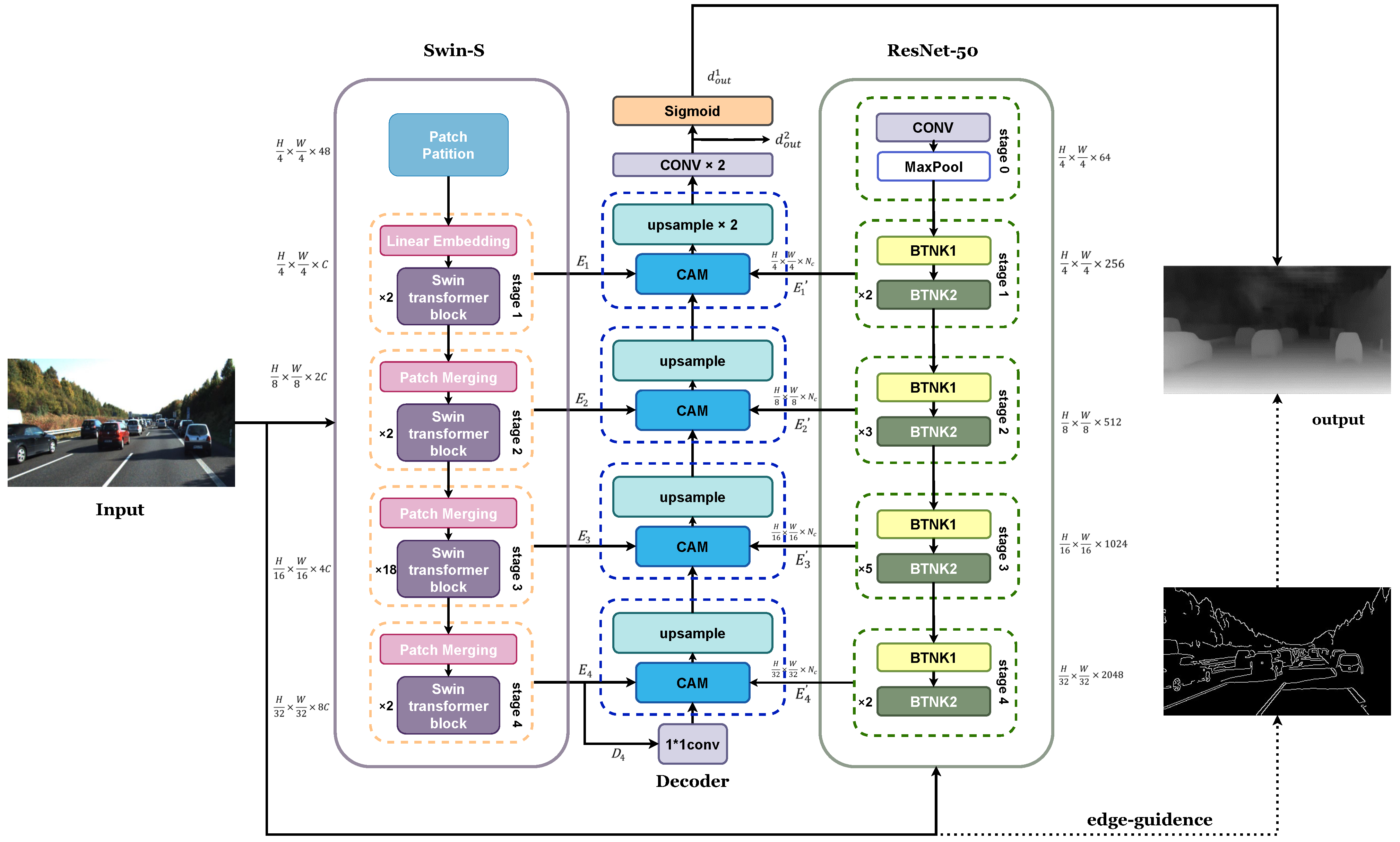
where i denotes the index value for each pixel in the input image, $p_i^{\ast }$ in the range [0, 1] represents the maximum depth probability for each pixel in the input image, $d_{\max }$ denotes the maximum depth of the scene corresponding to the predicted image in meters, and $y_i^{\ast }$ indicates the predicted depth value for each pixel. The model predicts the maximum depth probability map corresponding to the input image, which, when multiplied by the scene’s maximum depth value, yields the predicted depth map. This approach optimizes depth estimation by utilizing the relative depth relationships among pixels rather than directly predicting the absolute depth value of each pixel. The structure of EDPNet is shown in Figure 4.

The decoder alternates between placing CAM modules and upsampling modules to produce the final depth map output, as shown in Figure 5. The encoded feature $E_4$ from Swin Transformer first passes through a $1\times 1$ convolution to reduce the channel dimension to a fixed value $N_c$, resulting in the decoded feature $D_4$. The process goes through four stages; each stage has its input encoding and decoding feature maps represented by $E_i$, $E_i^{\prime }$, and $D_i$, respectively. The output feature map of each stage is represented by $D_{(i-1)}$, where i represents the order of the four stages from bottom to top; i can take values from 1 to 4 inclusive.

Each stage consists of a CAM and an upsampling module, where the CAM outputs a feature map of the same resolution as its input, and the upsampling module increases the resolution of the feature map by $2\times$ through bilinear interpolation. To achieve a lightweight decoder, the channel dimension of the feature maps during the decoding stage is always $N_c$, set to 64. After the fourth stage, a feature map of size $H/4\times W/4\times N_c$ is produced. This map then goes through two upsampling modules, two convolutional layers, and a sigmoid function. The result is a maximum depth probability map for each pixel, where the score at each pixel represents the probability of maximum depth. The final depth map is obtained according to Equation (8), allowing for continuous depth estimation at each pixel. The specific structure of the CAM is shown in Figure 5. The module employs a window-based multi-head cross-attention W-MCA mechanism to calculate the self-similarity between encoding and decoding features. This effectively merges both global and local features. The features $E_i$ and $E_i^{\prime }$ from the two encoder branches are first concatenated at the channel level, then processed through a $3\times 3$ convolutional layer to adjust the channel dimension to $N_c$, matching the decoding feature $D_i$.

After performing the convolutional operation, we obtain the query matrix $Q_w^d$ from $D_i$ using the weight matrix $W^Q$. Similarly, the key matrix $K_w^e$ and value matrix $V_w^e$ are obtained from $E_i$ and $E_i^{\prime }$ using the weight matrices $W^K$ and $W^V$, respectively. The cross-attention between the encoding and decoding features is then calculated within the partitioned windows. We first partition $Q_w^d$, $K_w^e$, and $V_w^e$ into windows of size $M\times M$, where M is set to 7. Next, we compute the cross-attention, and after that we calculate the multi-head cross-attention. The feature map is then passed through the MLP, LN layers, and a residual connection before being output to an upsampling module that enhances the spatial resolution. In summary, the entire computational process of the CAM can be described as follows:

$$Q_w^d=\mathrm{LN}\left(D_i\right)$$

(9)

$$K_w^e=\mathrm{LN}\left({\mathrm{Conv}}_{3\times 3}(E_i\otimes E_i^{\prime })\right)$$

(10)

$$V_w^e=\mathrm{LN}\left({\mathrm{Conv}}_{3\times 3}(E_i\otimes E_i^{\prime })\right)$$

(11)

$$L_i=\mathrm{W}-\mathrm{MCA}(Q_w^d,K_w^e,V_w^e)+D_i$$

(12)

$$\mathrm{W}-\mathrm{MCA}(Q_w^d,K_w^e,V_w^e)=\mathrm{softmax}\left(\frac{Q_w^d{\left(K_w^e\right)}^T}{\sqrt{d_k}}+B\right)V_w^e$$

(13)

$$L_i^{\prime }=\mathrm{MLP}\left(\mathrm{LN}\left(L_i\right)\right)+L_i$$

(14)

where ⊗ denotes channel-wise concatenation of $E_i$ and $E_i^{\prime }$, $L_i$ and $L_i^{\prime }$ represent, respectively, the feature maps input into the second LN layer and the output of the CAM. The dimensionality of the key vectors is represented by $d_k$. The learnable matrix B represents the relative positional embeddings between each query matrix and key matrix. After computing the cross-attention for all windows, the windows are rearranged and placed according to their spatial positions in the image.

3.3. Loss Function

3.3.1. Loss for Depth Prediction Error

The Berhu loss function is presented as a piecewise function that effectively constrains the depth prediction errors at different scales. The specific expression of the function is as follows:

$$B(d_i^{\ast }-d_i)=\left\{\begin{array}{cc}|d_i^{\ast }-d_i|\hfill & \mathrm{if}|d_i^{\ast }-d_i|\le c\hfill \\ \frac{{(d_i^{\ast }-d_i)}^2+c^2}{2c}\hfill & \mathrm{if}|d_i^{\ast }-d_i|>c\hfill \end{array}\right.$$

(15)

Here, $d_i^{\ast }$ and $d_i$ denote the depth prediction and the actual value for the ith pixel point, respectively, and i is the index of pixels in all images of each batch during the training process; c is a threshold. When the depth prediction error is less than or equal to the preset threshold c the Berhu loss function behaves as an L1 loss, which is straightforward and facilitates effective backpropagation of gradients. Conversely, when the error exceeds the threshold, the function transitions to an L2 loss, increasing the gradient values with the error to mitigate the vanishing gradient problem. Set $c=0.2{max}_i|d_i^{\ast }-d_i|$.

To optimize multi-scale depth prediction results, we designed a corresponding full-resolution multi-scale loss function based on the Berhu loss function. This function guides the optimization of feature maps at different stages of the decoder towards the same goal, thereby alleviating issues of detail loss and object edge blurring. The expression of the full-resolution multi-scale loss function is

$$L_{multi}=\left\{\begin{array}{cc}\frac{1}{N_s}\sum _{i=1}^{N_s}|d_i^{\ast }-d_i|\hfill & \mathrm{if}|d_i^{\ast }-d_i|\le c\hfill \\ \frac{1}{2N_s·c}\sum _{i=1}^{N_s}[{(d_i^{\ast }-d_i)}^2+c^2]\hfill & \mathrm{if}|d_i^{\ast }-d_i|>c\hfill \end{array}\right.$$

(16)

Here, $L_{multi}$ represents the loss corresponding to the two output results $d_{out}^s$, with $N_s$ being the number of pixels for the corresponding output results, and $s\in \{1,2\}$.

3.3.2. Loss for Punishing Depth Prediction Error on Edges of Objects

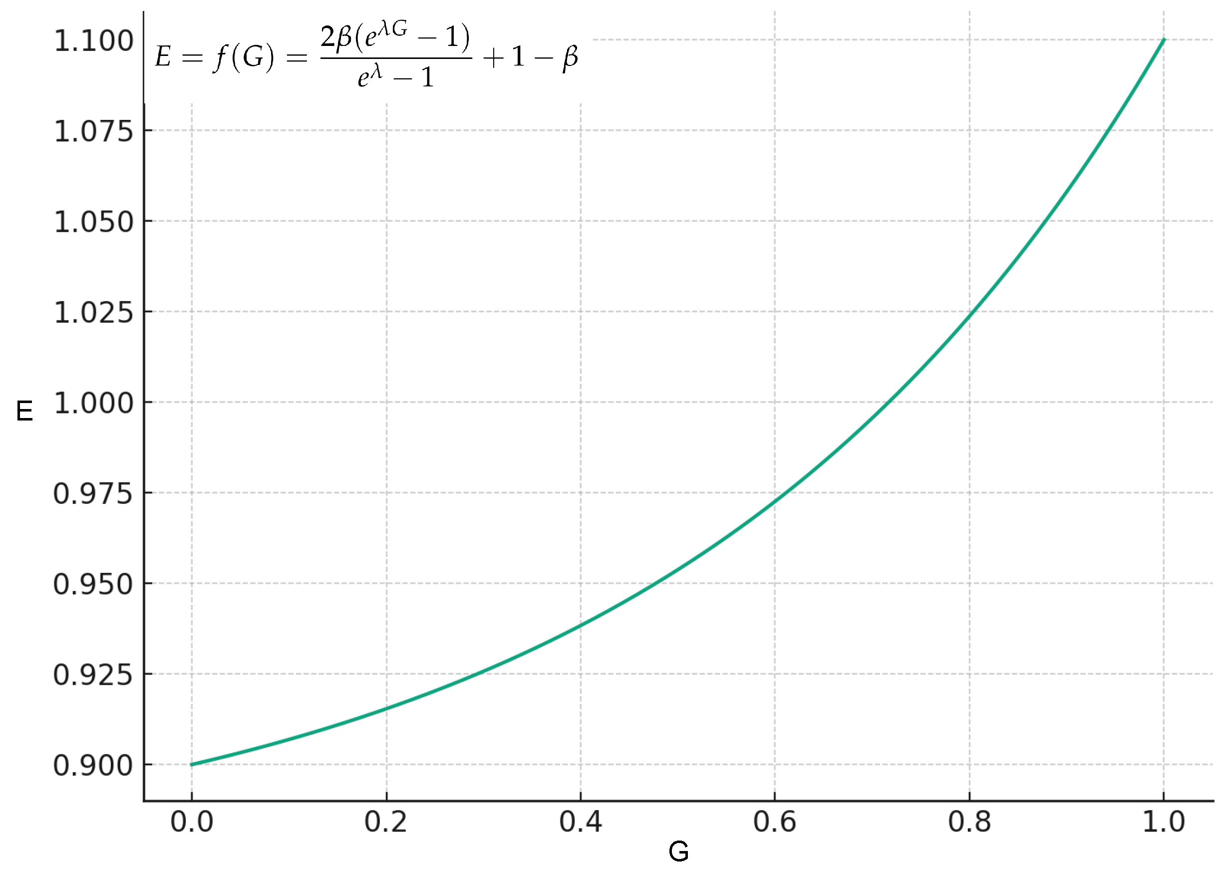
Edge information is an important clue for predicting depth [30]. To address the blurred edges and sparse data in training datasets leading to incomplete object boundaries and artifacts in predicted depth maps, we designed an edge-guided branch and edge-guided coefficient E to direct the variation of the loss function $L_{multi}$. When the gradient is close to 0, the edge-guided branch identifies the region as non-edge, reducing the penalty strength of the loss function; when the gradient approaches 1, the region is identified as an edge, increasing the penalty strength of the loss function.

First, the edge-guided branch calculates the gradient result for each pixel using the Sobel operator and normalizes it:

$$G=\left(\right|{\nabla }_x|+|{\nabla }_y\left|\right)/255$$

(17)

The edge-guided coefficient E varies with G as follows, as shown in Figure 6:

$$E=f\left(G\right)=\frac{2\beta (e^{\lambda G}-1)}{e^{\lambda }-1}+1-\beta$$

(18)

where, as G increases from 0 to 1, E gradually increases from $1-\beta$ to $1+\beta$, set $\beta =0.1,\lambda =2$:

$$L_{edge}=E·L_{multi}=\left\{\begin{array}{cc}\frac{1}{N_s}\sum _{i=1}^{N_s}|d_i^{\ast }-d_i|·E\hfill & \mathrm{if}|d_i^{\ast }-d_i|\le c\hfill \\ \frac{1}{2N_s·c}\sum _{i=1}^{N_s}[{(d_i^{\ast }-d_i)}^2+c^2]·E\hfill & \mathrm{if}|d_i^{\ast }-d_i|>c\hfill \end{array}\right.$$

(19)

By calculating losses at each level, we form an integrated edge-enhanced multi-scale loss function, denoted as $L_{all}$:

$$L_{all}=m\sqrt{\sum _{s=1}^2{\omega }_s{L}_{edge}}$$

(20)

where $L_{all}$ is the overall constraint during the training process, ${\omega }_s$ are the multi-scale weight coefficients, and m is a scaling factor. Setting an appropriate scaling factor can accelerate network training and allow for faster convergence. Set $m=10$.

By adopting an innovative edge-enhanced multi-scale loss function design, not only is global prediction accuracy focused on, but also the capture and optimization of local details are emphasized. This ensures that features at different scales are effectively learned. By integrating guidance from edge information, the model’s ability to detect object contours is enhanced. This improves the loss function in regions with edges but no depth, and boosts learning in areas with both edges and depth, which leads to a clearer distinction between recognized depth map boundaries.

4. Experiments

For this section, we conducted experimental testing and comparative evaluation of the EDPNet algorithm. Firstly, we will introduce the evaluation criteria adopted by this algorithm, as well as the datasets used for training and testing, and the detailed experimental settings. Then, we detail how we quantitatively and qualitatively assessed and compared the EDPNet algorithm with other typical methods, and, finally, how we tested the effectiveness of the key modules of the algorithm through ablation experiments.

4.1. Evaluation Index

In the field of monocular depth estimation, error and accuracy are commonly used for evaluation because they directly reflect the model’s performance in predicting depth from a single image, focusing on the core challenge of accurately capturing the 3D structure of a scene. Error metrics include absolute relative error, square relative error, root mean squared error, and root mean squared logarithmic error. Accuracy metrics include accuracy under three different threshold values. In monocular depth estimation, the primary task is to infer the distance of objects from the camera, which inherently involves understanding the scene’s geometry. Accuracy measures how close the estimated depths are to the true depths, while error metrics (like absolute relative error, squared relative error, RMSE) specifically quantify the deviation of estimated depth values from Ground Truth values across the dataset. These metrics directly address the problem’s geometric nature by assessing the precision of depth values, which is crucial for applications requiring accurate 3D reconstructions. We assume that the total number of pixels in all evaluated images is N, and that $d_i^{\ast }$ and $d_i$ are the predicted and true depth values of pixel i, respectively, where $0\le i\le N-1$.

Absolute relative error (AbsRel): As a dimensionless metric, this is used to evaluate the average relative deviation between all pixels’ depth prediction values and their actual values in an image. This reflects the average accuracy of predicted depth values, calculated as the average of the absolute value of the difference between predicted depths and actual depths relative to the actual depths. This metric is commonly utilized to gauge the performance of depth prediction models, especially in their ability to accurately capture the three-dimensional structure of a scene, as indicated in Equation (21):

$$\mathrm{AbsRel}=\frac{1}{N}\sum _{i=1}^N\frac{|d_i^{\ast }-d_i|}{d_i}$$

(21)

Square Relative Error (SqRel): As a dimensional metric, this calculates the average of the ratio of the squared difference between the predicted depth values for all pixels and their true depth values to the true depth values. This metric places more emphasis on the impact of large errors. By analyzing this metric, depth prediction models can be more effectively evaluated and improved upon, particularly in their performance on areas with significant depth variations. The formula is as shown in Equation (22):

$$\mathrm{SqRel}=\frac{1}{N}\sum _{i=1}^N\frac{{(d_i^{\ast }-d_i)}^2}{d_i}$$

(22)

Root Mean Square Error (RMSE): RMSE measures the square root of the average of the squares of differences between the predicted and true depth values of all the pixels in the image. It assesses the dispersion of depth values between the predicted depth map and the Ground Truth (GT) depth map. The formula is as shown in Equation (23):

$$\mathrm{RMSE}=\sqrt{\frac{1}{N}\sum _{i=1}^N{(d_i^{\ast }-d_i)}^2}$$

(23)

Root Mean Square Logarithmic Error (RMSElog): RMSElog applies a logarithmic transformation to the depth values in the RMSE metric, reducing the impact of larger errors on the standard deviation. The formula is as shown in Equation (24):

$$\mathrm{RMSElog}=\sqrt{\frac{1}{N}\sum _{i=1}^N{[log\left(d_i^{\ast }\right)-log\left(d_i\right)]}^2}$$

(24)

Accuracy: Accuracy is calculated by counting the number of pixels in the image for which the ratio of the predicted depth value to the true depth value, and its inverse, have their maximum within a specified threshold range. The ratio of the number of these pixels within the threshold range to the total number of pixels in the image represents the accuracy. The specific formula is as shown in Equation (25):

$$\mathrm{Accuracy}=\frac{1}{N}\sum _{i=1}^N[max(\frac{d_i^{\ast }}{d_i},\frac{d_i}{d_i^{\ast }})<\delta ]$$

(25)

Here, $\delta$ is the accuracy threshold, with ${\delta }_1=1.25$, ${\delta }_2=1.{25}^2$, and ${\delta }_3=1.{25}^3$ being used in this context. Among these evaluation metrics for assessing the quality of monocular image depth estimation algorithms, higher accuracy indicates better performance, while lower values for the other metrics also indicate better performance.

4.2. Datasets

Training on high-quality datasets is crucial for enhancing the performance of network models, and this is also true for monocular image depth estimation tasks. Several research institutions have released datasets for MDE, which vary in scene types and depth ranges. This section will focus on the commonly used NYU Depth V2 [9], KITTI [10], and SUN RGB-D [11].

4.2.1. NYU Depth V2 Dataset

The NYU Depth V2 dataset [9] is the most frequently used indoor scene dataset in the field of monocular image depth estimation and serves as the primary training dataset for supervised methods. It was created by Silberman et al. using a Kinect depth camera to collect color images and corresponding depth maps from 464 scenes, comprising approximately 120,000 RGB-depth image pairs. Out of these, images from 249 scenes are used for training, while images from 215 scenes are utilized for testing. The RGB images have a resolution of 640 × 480, and the true depth range of the entire dataset spans from 0.5 m to 10 m. Additionally, the authors employed a coloring algorithm to fill in 1449 depth maps, resulting in densely aligned image pairs. These 1449 image pairs are divided into a training set of 795 pairs and a test set of 654 pairs.

4.2.2. SUN RGB-D Dataset

The SUN RGB-D dataset [11] is a large-scale benchmark dataset constructed by Song et al., featuring rich scene diversity. This dataset was captured using four different RGB-D depth cameras, comprising color images and corresponding depth maps from 10,335 real indoor scenes. The entire dataset is densely annotated by humans, including object categories, two-dimensional shapes, and three-dimensional spatial layouts. Of these images, 5285 are designated for training and 5050 for testing, with a depth limit of up to 10 m.

4.2.3. KITTI Dataset

The KITTI dataset [10] is one of the most commonly used outdoor-scene datasets in the field of computer vision. It also serves as the most prevalent benchmark dataset for unsupervised/semi-supervised monocular image depth estimation methods. This dataset was collected by Geiger et al. using a mobile platform equipped with two color cameras (FL2-14S3C-C), two grayscale cameras (FL2-14S3M-C), one Velodyne HDL-64E rotating 3D laser scanner, and a OXTS RT3003 inertial and GPS navigation system, with a maximum measurement distance of 120 m. It comprises images from 61 different outdoor scenes, totaling approximately 93,000 RGB-depth image pairs. Images from 32 scenes are used for training, while images from 29 scenes are used for testing. The original RGB images have a resolution of 1242 × 375.

4.3. Implementation Details

EDPNet was developed on the Ubuntu-18.04 operating system utilizing the PyTorch 1.5.1 framework to construct a dual-stream encoder–decoder network architecture. Aside from the two encoder branches, the rest of the network parameters were initialized using the Xavier method. During the training phase, the batch size was set to eight, with the Adam optimizer for adjustments, where ${\beta }_1=0.9$, ${\beta }_2=0.999$, and $ϵ={10}^{-8}$. Following the approach of Bhat et al., a $1Cycle$ learning rate decay method was used, with the initial learning rate for the Swin Transformer encoder branch set at $6\times {10}^{-5}$ and for the ResNet-50 encoder branch set at ${10}^{-4}$. A linear strategy was used to adjust the learning rate for the first 30% of iterations, followed by a cosine strategy for learning rate decay, with the total cycle set to 80 epochs. Training was conducted on a system equipped with a dual-channel 32GiB memory i7-7800X processor and two NVIDIA GeForce GTX 1080Ti graphics cards with 11GiB of VRAM each. All the hyperparameters are in

Table 1. EDPNet model hyperparameters.

Hyperparameter	Value
Hardware Configuration	i7-7800X CPU, 32GiB RAM, 2x NVIDIA GTX 1080Ti
Operating System	Ubuntu-18.04
Framework	PyTorch
Parameter Initialization	Xavier method
Batch Size	8
Total Epochs	80
Optimizer	Adam ${\beta }_1=0.9$, ${\beta }_2=0.999$, $ϵ={10}^{-8}$
Learning Rate Decay Method	$1Cycle$
Initial Learning Rate for Swin Transformer	$6\times {10}^{-5}$
Initial Learning Rate for ResNet-50	${10}^{-4}$
Learning Rate Adjustment Strategy	30% warm-up, 70% cosine strategy rate decay

.

The algorithm was trained and tested on NYU Depth V2 [9], KITTI [10]. To alleviate overfitting and enhance the generalizability of EDPNet to real-world scenarios, data augmentation techniques were employed to expand the training set. These techniques included: (1) Random horizontal flipping: training RGB images were horizontally flipped, with a 50% probability. (2) Random color transformation: the channel values of training RGB images were randomly multiplied by a scaling factor ranging from 0.8 to 1.2. (3) Random rotation: training images were rotated around an axis passing through the image center and perpendicular to the image plane. The rotation angles ranged between −2.5° and 2.5° for the NYU Depth V2 dataset and between −1° and 1° for the KITTI dataset.

Additionally, to verify the proposed algorithm’s generalization capability across various scene types, for this chapter we conducted zero-shot cross-dataset evaluation experiments on the diverse SUN RGB-D dataset. The EDPNet model was trained on the NYU Depth V2 dataset without any fine-tuning, then evaluated on the SUN RGB-D dataset for its depth estimation performance. Compared to training and testing the model on subsets of the same dataset, the results from the zero-shot cross-dataset evaluation more accurately represent the proposed model’s depth estimation capabilities in real-world scenarios.

In all the evaluation experiments, the depth maps predicted by the network were readjusted to match the median depth with that of the Ground Truth. Moreover, the final output depth map was calculated by averaging the prediction results of an image and its mirrored image, ensuring accuracy and consistency in depth estimation.

4.4. Experimental Results and Analysis

In order to ensure objectivity and fairness, the index calculation methods we used were all common methods in the field, and the parameters of the comparison model were all taken from the best results given in their original papers.

4.4.1. Analysis of the Results of the Indoor Dataset NYU DepthV2

The NYU Depth V2 dataset is widely used to evaluate depth estimation models, due to its diverse indoor scenarios. Based on the NYU Depth V2 dataset, for this section we conducted quantitative and qualitative analysis of various supervised monocular depth estimation methods. The quantitative and qualitative analysis is shown in

Table 2. The index calculation results on the NYU Depth V2 dataset.

Methods	Error			Accuracy
	AbsRel↓	RMSE↓	RMSElog↓	${\mathit{\delta }}_{\mathbf{1}}$↑	${\mathit{\delta }}_{\mathbf{2}}$↑	${\mathit{\delta }}_{\mathbf{3}}$↑
Make3d [31]	0.349	1.214	-	0.447	0.745	0.897
Eigen [7]	0.158	0.641	0.214	0.769	0.950	0.988
Laina [32]	0.127	0.573	0.195	0.811	0.953	0.988
GeoNet [20]	0.128	0.569	-	0.834	0.960	0.990
DORN [22]	0.115	0.509	-	0.828	0.965	0.992
SharpNet [33]	0.139	0.502	0.157	0.836	0.966	0.993
BTS [34]	0.110	0.392	0.142	0.885	0.978	0.994
Yin [35]	0.108	0.416	0.148	0.875	0.976	0.994
DenseDepth [16]	0.103	0.390	-	0.895	0.980	0.996
DAV [36]	0.108	0.412	-	0.882	0.980	0.996
TransDepth [37]	0.106	0.365	-	0.900	0.983	0.996
SwinDepth [26]	0.100	0.354	0.042	0.909	0.986	0.997
Adabins [23]	0.103	0.364	-	0.903	0.984	0.997
EDPNet	0.099	0.363	0.121	0.903	0.986	0.997

The bolded part is the best.

and Figure 7:

The quantitative experimental analysis indicated improvements across all metrics with our proposed algorithm. SwinDepth employs the Swin Transformer architecture, which effectively captures long-distance dependencies through its adaptive window mechanism, which optimizes the integration of global contextual information. Although SwinDepth demonstrates excellent performance in depth estimation tasks, its ability to capture details, especially in edge regions, may not match that of EDPNet. On the other hand, the Adabins method estimates depth by dividing images into different adaptive bins, utilizing an innovative approach to improve the granularity and accuracy of depth predictions. Additionally, it uses a small Transformer network to predict interval sizes and achieves better depth estimation. While Adabins is highly effective in enhancing the granularity of depth estimates, it may not capture global context and long-distance dependencies as well as Transformer-based models. The EDPNet method we have introduced combines the ability to model long distances and enhance edge information, ensuring the integration of global contextual information and the reproduction of high-quality edge details in indoor depth estimation tasks. It better understands the boundaries and details of objects within indoor scenes, thereby providing more precise and refined depth predictions.

4.4.2. Analysis of the Results of the Outdoor Dataset KITTI

The KITTI dataset, widely utilized for evaluating depth estimation models, due to its real-world driving scenarios, served as the basis for our quantitative and qualitative analyses of the various supervised monocular depth estimation methods. The quantitative results are displayed in

Table 3. The index calculation results on the KITTI dataset.

Methods	Error			Accuracy
	AbsRel↓	RMSE↓	RMSElog↓	${\mathit{\delta }}_{\mathbf{1}}$↑	${\mathit{\delta }}_{\mathbf{2}}$↑	${\mathit{\delta }}_{\mathbf{3}}$↑
Make3d [31]	0.280	8.734	0.361	0.601	0.820	0.926
Eigen [7]	0.203	6.307	0.282	0.702	0.898	0.967
Liu [12]	0.201	6.471	0.273	0.680	0.898	0.967
Garg [38]	0.169	5.104	0.273	0.740	0.904	0.962
Monodepth2 [39]	0.106	4.630	0.193	0.876	0.958	0.980
DORN [22]	0.072	2.727	0.120	0.932	0.984	0.994
Yin [35]	0.072	3.258	0.117	0.938	0.990	0.998
GAN [40]	0.098	3.933	0.173	0.890	0.964	0.985
SharpNet [33]	0.093	2.727	0.120	0.886	0.965	0.986
BTS [34]	0.060	2.798	0.096	0.955	0.993	0.998
TransDepth [37]	0.064	2.755	0.098	0.956	0.994	0.999
SwinDepth [26]	0.064	2.643	0.097	0.957	0.994	0.999
DPT [41]	0.062	2.573	0.092	0.959	0.995	0.999
AdaBins [23]	0.058	2.360	0.088	0.964	0.995	0.999
EDPNet	0.057	2.357	0.089	0.964	0.995	0.999

The bolded part is the best.

, assessing the accuracy and robustness of depth estimation methods. The qualitative findings are illustrated in Figure 8, vividly highlighting the capabilities of depth estimation in complex outdoor environments.

The experimental results indicate that the approaches discussed in this chapter achieve better outcomes in the majority of outdoor scenarios. Notably, the Dense Prediction Transformer (DPT) method, which utilizes Vision Transformer as its backbone network, demonstrates impressive performance in outdoor scenes. This suggests that Transformer’s handling of global information surpasses that of convolutional networks in efficacy. Furthermore, the AdaBins network surpasses the network proposed in this chapter, in terms of RMSElog, indicating that the AdaBins method’s adaptive bins technique contributes to refining the precision and accuracy of depth prediction. However, it is still evident from the visualization results that our algorithm significantly enhances edge details.

4.4.3. Analysis of the Results of the Dataset SUN RGB-D

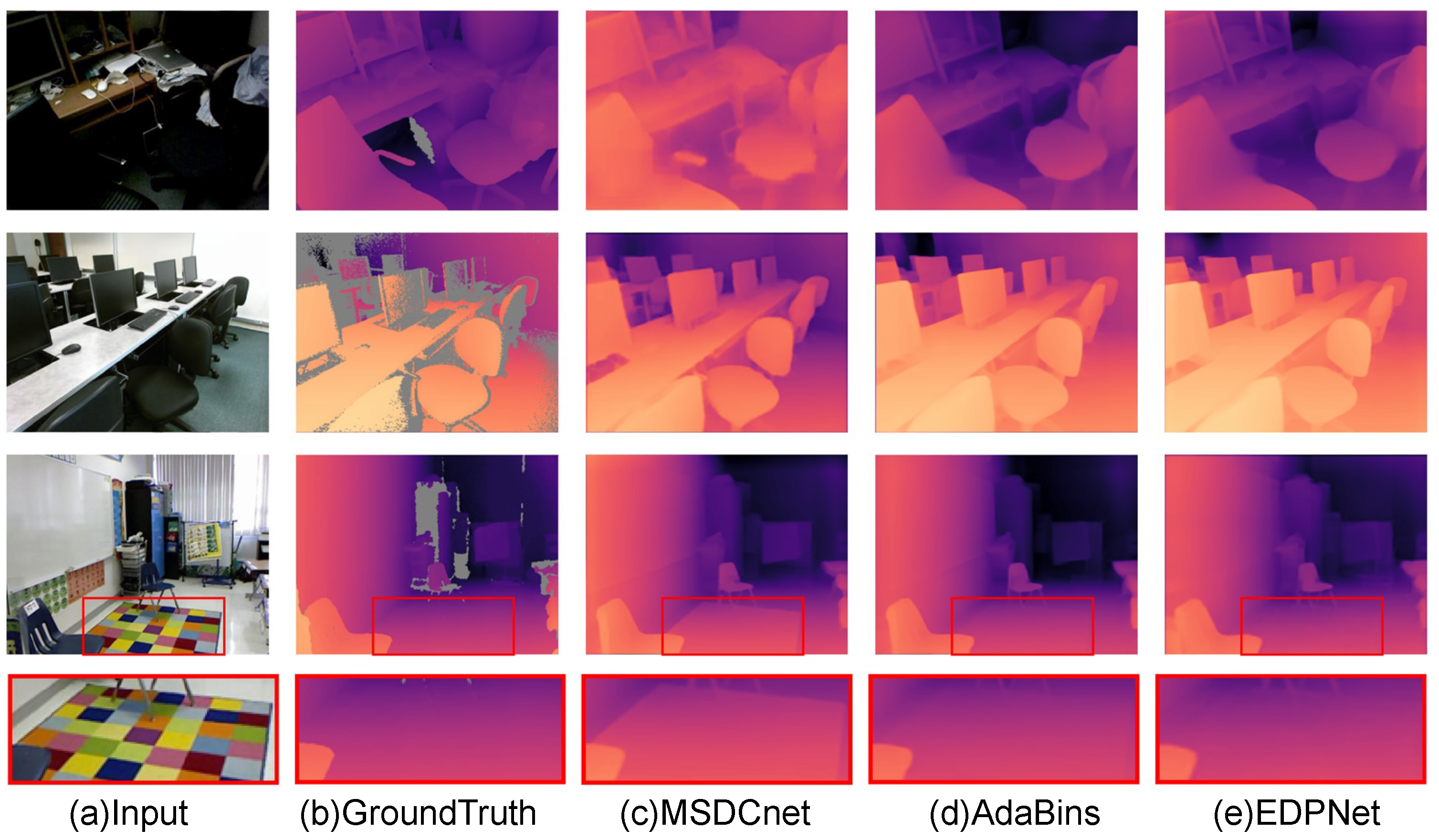
The SUN RGB-D dataset contains a vast array of RGB-D images from various indoor environments, encompassing a wide range of scene types, providing a challenging test platform for depth estimation models. For this section, we evaluated the EDPNet model’s generalization capability by training it on the NYU Depth V2 dataset and then testing it directly on the SUN RGB-D dataset without further training, assessing its adaptability to unseen scenes. The quantitative analysis results are presented in

Table 4. The index calculation results on the SUN RGB-D dataset.

Methods	Error			Accuracy
	AbsRel↓	RMSE↓	RMSElog↓	${\mathit{\delta }}_{\mathbf{1}}$↑	${\mathit{\delta }}_{\mathbf{2}}$↑	${\mathit{\delta }}_{\mathbf{3}}$↑
Chen [28]	0.166	0.494	-	0.757	0.943	0.984
Yin [35]	0.183	0.541	-	0.696	0.912	0.973
BTS [34]	0.172	0.515	-	0.740	0.933	0.980
AdaBins [23]	0.159	0.476	-	0.771	0.944	0.983
EDPNet	0.156	0.478	0.158	0.780	0.948	0.986

The bolded part is the best.

, while the qualitative analysis findings are depicted in Figure 9.

Based on the results obtained on the SUN RGB-D dataset, it is evident that our EDPNet performs exceptionally well in terms of generalization. Compared to other network methods, it yields depth results that are closer to the Ground Truth. Despite the fact that AdaBins attempted to alleviate edge issues by embedding a mini-ViT behind the decoder, depth artifacts still occurred. The core idea of the AdaBins algorithm is to adaptively divide the depth range into multiple bins. By dynamically adjusting these depth bins, AdaBins can adaptively improve the accuracy of depth estimation based on the content of the image, which enhances the precision in the details of the generated depth maps. Although AdaBins shows good performance in terms of detail and depth accuracy in many scenarios, its generalization performance is still not strong enough. On the other hand, the method in this paper produces clearer results, particularly for RGB images with edges that lack depth, such as carpets. The edge guidance branch is effective in guiding the network model to ensure that the predicted depth maps are not affected by carpet patterns.

4.5. Ablation Study

To validate the effectiveness of the modules proposed in this paper, we designed the following ablation studies to analyze and compare the performance of each module: (1) evaluating the dual encoder branches, to analyze the impact of image features extracted by different encoders on performance; (2) assessing different feature fusion methods, to examine the effect of the Cross-Attention Module on depth estimation; (3) evaluating various loss functions, to analyze the rationale behind the designed edge-enhanced multi-scale loss function.

4.5.1. Comparison of Different Backbones

To validate the generalization capability of the dual-stream framework, we further explored the performance of different backbone architectures in the dual-stream branches to ascertain whether various scales of ResNet and Swin Transformer versions are compatible with our proposed framework. We conducted experiments using the widely used ResNet50 and Swin-S architectures, and compared them to four other network architectures. The objective was to gain a deeper understanding of how various backbone network architectures specifically affect the performance of the dual-stream framework, with the experimental results presented in

Table 5. Comparison of Different Backbones on NYU Depth V2.

Backbone		Params	Error		Accuracy
ResNet	Swin		AbsRel↓	RMSE↓	${\mathit{\delta }}_{\mathbf{1}}$↑	${\mathit{\delta }}_{\mathbf{2}}$↑	${\mathit{\delta }}_{\mathbf{3}}$↑
ResNet50	Swin-B	156M	0.097	0.362	0.904	0.987	0.997
ResNet101	Swin-S	133M	0.098	0.362	0.903	0.987	0.997
ResNet50	Swin-S	113M	0.099	0.363	0.903	0.986	0.997
ResNet50	Swin-T	92M	0.110	0.435	0.866	0.976	0.995

The bolded part is the best.

:

Analyzing the experimental data revealed that despite Swin-T and ResNet having fewer structural parameters, their performance significantly decreased, falling behind other architectures in all metrics. In contrast, while Swin-B had the highest number of parameters, its performance was comparable to Swin-S, with no significant improvement. The comparative study between ResNet101 and ResNet50 shows that although an increase in parameters led to some performance enhancement, the improvement was not substantial. In the practical application of monocular depth estimation, both efficiency and accuracy are crucial factors. Hence, when seeking a balance between parameters and performance, the combination of ResNet50 and Swin-S demonstrates superior efficacy.

4.5.2. Comparison of Feature Fusion Methods

To validate the efficacy of both encoding pathways on the network’s outcome and the decoder’s ability to more effectively integrate the multi-scale features from the dual-stream encoder, for this section we began by isolating the ResNet encoder and the Transformer encoder as bases. The decoder initially utilized standard convolutional layers and bilinear upsampling layers, followed by the application of the Cross-Attention Module designed in this work for feature fusion. Through comparing the errors and accuracies of the various models, the objective was to deeply understand the influence of each component on performance. The design of the ablation experiments is presented in

Table 6. Comparison of feature fusion methods on NYU Depth V2.

Method	Encoder		CAM	Error		Accuracy
	ResNet	Swin		AbsRel↓	RMSE↓	${\mathit{\delta }}_{\mathbf{1}}$↑	${\mathit{\delta }}_{\mathbf{2}}$↑	${\mathit{\delta }}_{\mathbf{3}}$↑
1	✓	×	×	0.145	0.588	0.815	0.958	0.990
2	×	✓	×	0.134	0.532	0.854	0.967	0.993
3	✓	✓	×	0.142	0.576	0.834	0.966	0.992
4	✓	✓	✓	0.110	0.385	0.887	0.979	0.995

The bolded part is the best.

, where Method 1 employed only ResNet as a single encoder branch, and Method 2 utilized only the SwinTransformer as a single encoder branch, with both Methods 1 and 2’s decoders implementing convolution and bilinear upsampling. Method 3 engaged both encoding branches, adding skip connections between the encoder and decoder and using a simple Concat-Conv for feature fusion. Method 4 concurrently employed the encoding branches and utilized the designed Cross-Attention Module to integrate shallow decoder features with encoder features.

The results from the four methods depicted in the figures suggest that when the ResNet encoding branch was used independently, the depth maps generated by the network exhibited relatively high errors, indicating that the model’s effectiveness was not particularly ideal. In contrast, when switching to the independent SwinTransformer branch, the network showed significant improvements across various metrics. This suggests that for complex indoor scenes, modeling long-distance relationships by incorporating global information yields better encoding performance than using ResNet, resulting in superior depth information restoration. However, simply concatenating and convolving features from the dual-path encoders led to deteriorated network performance. This degradation was attributable to the independent operation of the two encoder branches, each extracting image features with distinct semantics. Merely concatenating these features resulted in insufficient feature fusion and mismatches, where corresponding features were inappropriately merged. After incorporating a feature fusion encoder with cross-attention, the network performance improved compared to using individual branches. This indicates that the designed feature fusion module effectively bridges the semantic gap between encoding and decoding features, efficiently aggregates multi-scale features, and provides critical information for the decoder to restore depth maps. Furthermore, the two branches of the encoder are indeed complementary, enhancing global information modeling and local detail retention.

4.5.3. Comparison of the Loss Function

To validate the effectiveness of the edge depth prediction error penalization loss proposed in this paper, we compared the results using the basic full-resolution multi-scale loss function (named as Method M) with those using the proposed edge-enhanced loss function (named as Method E) in ablation experiments, as shown in

Table 7. Comparison of the loss function on NYU Depth V2.

Methods	Loss	Error		Accuracy
		AbsRel↓	RMSE↓	${\mathit{\delta }}_{\mathbf{1}}$↑	${\mathit{\delta }}_{\mathbf{2}}$↑	${\mathit{\delta }}_{\mathbf{3}}$↑
1	M	0.110	0.385	0.887	0.979	0.995
2	E	0.099	0.363	0.903	0.986	0.997

The bolded part is the best.

:

Analyzing the ablation experiment results, we arrived at the following conclusions: Method E exhibited a lower AbsRel error, indicating that the edge information loss function provides depth predictions closer to the actual depth values, reflecting higher prediction accuracy. Furthermore, a lower RMSE value for Method E suggests an overall improvement in the precision of depth prediction. Additionally, Method E outperformed Method M across the three accuracy metrics ${\delta }_1$, ${\delta }_2$, ${\delta }_3$, demonstrating the edge-information-enhanced loss function’s significant advantage in maintaining consistency between predicted and actual depths, especially within more lenient proportional ranges. In summary, the edge-enhanced loss function (Method E) significantly improves the precision and accuracy of depth prediction by incorporating edge information into the loss function. These improvements are evident across the key metrics of AbsRel error, RMSE, and accuracy indicators, enhancing the model’s sensitivity and predictive capability regarding depth edges. This leads to depth estimations that are more closely aligned with real-world scenarios. This method is particularly valuable for depth prediction tasks, as it substantially enhances the quality and reliability of depth estimations.

To intuitively demonstrate the effectiveness of the edge enhancement loss function proposed, for this section we selected a set of indoor scenes rich in object edges for an ablation study of the effects. The “M method” displays the results using a full-resolution multi-scale loss function, while the “E method” shows the results of employing an edge enhancement loss function to strengthen the depth information. The experimental results are illustrated in Figure 10.

From the details in the figures, it is evident that the loss function proposed effectively enhances the depth restoration of object edges in scenes. The depth at the edges of objects within the red and green frames is noticeably enhanced. For the box in the blue frame, which is easily overlooked due to being obscured, the depth was ignored by the original method. However, with the introduction of the edge loss enhancement by the E method, even easily overlooked objects are well-represented. In the green frame, the depth of areas with patterns and depth on the bottom is clearly identified, while the upper area with patterns but no depth did not generate artifacts. This proves that the network has indeed enhanced the recognition of true object edges, demonstrating the efficacy of our proposed method.

5. Conclusions

For this paper, we designed an encoding–decoding network framework that combines Swin Transformer and ResNet, leveraging the complementary characteristics of Vision Transformer and CNN to extract multi-scale contextual information. A multi-head cross-attention mechanism is employed to fuse features, alleviating the semantic gap between encoding and decoding features. Additionally, an edge-enhanced multi-scale loss function is utilized to strengthen loss at image edges, improving the model’s ability to recognize object contours. Extensive experiments on the NYU Depth V2 dataset, KITTI dataset, and SUN RGB-D dataset, along with lateral comparisons with other state-of-the-art methods and ablation studies of the model itself, demonstrate that EDPNet surpasses most monocular image depth estimation algorithms. It achieves accurate pixel-level depth estimation and possesses excellent generalization performance.

In the future, a consideration may be to reduce the number of network parameters and to decrease computational complexity through model compression methods, while maintaining high depth estimation accuracy to enhance practical application capabilities in tasks such as autonomous driving. Additionally, regarding the current issue of insufficient depth image datasets, semi-supervised or unsupervised methods can be used to overcome the dependency on datasets. Moreover, utilizing high-precision depth sensing equipment to construct larger-scale, higher-quality, and more diverse types of scene depth datasets holds profound significance.

References

- Han, J.; Shao, L.; Xu, D.; Shotton, J. Enhanced computer vision with microsoft kinect sensor: A review. IEEE Trans. Cybern. 2013, 43, 1318–1334. [Google Scholar] [PubMed]
- Bartczak, B.; Koch, R. Dense depth maps from low resolution time-of-flight depth and high resolution color views. In Proceedings of the International Symposium on Visual Computing, Las Vegas, NV, USA, 30 November–2 December 2009; Springer: Berlin/Heidelberg, Germany, 2009; pp. 228–239. [Google Scholar]
- Chan, K.-H.; Im, S.-K. Light-field image super-resolution with depth feature by multiple-decouple and fusion module. Electron. Lett. 2024, 60, e13019. [Google Scholar] [CrossRef]
- Shilian, Z.; Zhuang, Y.; Weiguo, S.; Luxin, Z.; Jiawei, Z.; Zhijin, Z.; Xiaoniu, Y. Deep Learning-Based DOA Estimation. IEEE Trans. Cogn. Commun. Netw. 2024, 1. [Google Scholar] [CrossRef]
- Rogister, P.; Benosman, R.; Ieng, S.H.; Lichtsteiner, P.; Delbruck, T. Asynchronous event-based binocular stereo matching. IEEE Trans. Neural Netw. Learn. Syst. 2011, 23, 347–353. [Google Scholar] [CrossRef] [PubMed]
- Koenderink, J.J.; Van Doorn, A.J. Affine structure from motion. JOSA A 1991, 8, 377–385. [Google Scholar] [CrossRef] [PubMed]
- Eigen, D.; Puhrsch, C.; Fergus, R. Depth map prediction from a single image using a multi-scale deep network. Adv. Neural Inf. Process. Syst. 2014, 27, 1–9. [Google Scholar]
- Li, Y.; Wei, X.; Fan, H. Attention Mechanism Used in Monocular Depth Estimation: An Overview. Appl. Sci. 2023, 13, 9940. [Google Scholar] [CrossRef]
- Silberman, N.; Hoiem, D.; Kohli, P.; Fergus, R. Indoor segmentation and support inference from rgbd images. In Proceedings of the Computer Vision–ECCV 2012: 12th European Conference on Computer Vision, Florence, Italy, 7–13 October 2012; Proceedings, Part V 12. Springer: Berlin/Heidelberg, Germany, 2012; pp. 746–760. [Google Scholar]
- Geiger, A.; Lenz, P.; Urtasun, R. Are we ready for Autonomous Driving? The KITTI Vision Benchmark Suite. In Proceedings of the Conference on Computer Vision and Pattern Recognition (CVPR), Providence, RI, USA, 16–21 June 2012. [Google Scholar]
- Song, S.; Lichtenberg, S.P.; Xiao, J. Sun rgb-d: A rgb-d scene understanding benchmark suite. In Proceedings of the IEEE Conference on Computer Vision and Pattern Recognition, Boston, MA, USA, 7–12 June 2015; pp. 567–576. [Google Scholar]
- Liu, F.; Shen, C.; Lin, G.; Reid, I. Learning depth from single monocular images using deep convolutional neural fields. IEEE Trans. Pattern Anal. Mach. Intell. 2015, 38, 2024–2039. [Google Scholar] [CrossRef] [PubMed]
- Li, B.; Shen, C.; Dai, Y.; Van Den Hengel, A.; He, M. Depth and surface normal estimation from monocular images using regression on deep features and hierarchical crfs. In Proceedings of the IEEE Conference on Computer Vision and Pattern Recognition, Boston, MA, USA, 7–12 June 2015; pp. 1119–1127. [Google Scholar]
- Duong, H.T.; Chen, H.M.; Chang, C.C. URNet: An UNet-Based Model with Residual Mechanism for Monocular Depth Estimation. Electronics 2023, 12, 1450. [Google Scholar] [CrossRef]
- Kim, I.S.; Kim, H.; Lee, S.; Jung, S.K. HeightNet: Monocular Object Height Estimation. Electronics 2023, 12, 350. [Google Scholar] [CrossRef]
- Alhashim, I.; Wonka, P. High quality monocular depth estimation via transfer learning. arXiv 2018, arXiv:1812.11941. [Google Scholar]
- Huang, G.; Liu, Z.; Van Der Maaten, L.; Weinberger, K.Q. Densely connected convolutional networks. In Proceedings of the IEEE Conference on Computer Vision and Pattern Recognition, Honolulu, HI, USA, 21–26 July 2017; pp. 4700–4708. [Google Scholar]
- Song, M.; Lim, S.; Kim, W. Monocular depth estimation using laplacian pyramid-based depth residuals. IEEE Trans. Circuits Syst. Video Technol. 2021, 31, 4381–4393. [Google Scholar] [CrossRef]
- Xie, S.; Girshick, R.; Dollár, P.; Tu, Z.; He, K. Aggregated residual transformations for deep neural networks. In Proceedings of the IEEE conference on Computer Vision and Pattern Recognition, Honolulu, HI, USA, 21–26 July 2017; pp. 1492–1500. [Google Scholar]
- Qi, X.; Liao, R.; Liu, Z.; Urtasun, R.; Jia, J. Geonet: Geometric neural network for joint depth and surface normal estimation. In Proceedings of the IEEE Conference on Computer Vision and Pattern Recognition, Salt Lake City, UT, USA, 18–23 June 2018; pp. 283–291. [Google Scholar]
- Jiao, J.; Cao, Y.; Song, Y.; Lau, R. Look deeper into depth: Monocular depth estimation with semantic booster and attention-driven loss. In Proceedings of the European Conference on Computer Vision (ECCV), Munich, Germany, 8–14 September 2018; pp. 53–69. [Google Scholar]
- Fu, H.; Gong, M.; Wang, C.; Batmanghelich, K.; Tao, D. Deep ordinal regression network for monocular depth estimation. In Proceedings of the IEEE Conference on Computer Vision and Pattern Recognition, Salt Lake City, UT, USA, 18–23 June 2018; pp. 2002–2011. [Google Scholar]
- Bhat, S.F.; Alhashim, I.; Wonka, P. Adabins: Depth estimation using adaptive bins. In Proceedings of the IEEE/CVF Conference on Computer Vision and Pattern Recognition, Nashville, TN, USA, 20–25 June 2021; pp. 4009–4018. [Google Scholar]
- Vaswani, A.; Shazeer, N.; Parmar, N.; Uszkoreit, J.; Jones, L.; Gomez, A.N.; Kaiser, Ł.; Polosukhin, I. Attention is all you need. Adv. Neural Inf. Process. Syst. 2017, 30, 1–11. [Google Scholar]
- Wang, W.; Tan, C.; Yan, Y. Monocular Depth Estimation Algorithm Integrating Parallel Transformer and Multi-Scale Features. Electronics 2023, 12, 4669. [Google Scholar] [CrossRef]
- Cheng, Z.; Zhang, Y.; Tang, C. Swin-Depth: Using Transformers and Multi-Scale Fusion for Monocular-Based Depth Estimation. IEEE Sens. J. 2021, 21, 26912–26920. [Google Scholar] [CrossRef]
- Chen, M.; Liu, J.; Zhang, Y.; Feng, Q. RA-Swin: A RefineNet Based Adaptive Model Using Swin Transformer for Monocular Depth Estimation. In Proceedings of the 2022 8th International Conference on Virtual Reality (ICVR), Nanjing, China, 26–28 May 2022; IEEE: Piscataway, NJ, USA, 2022; pp. 270–279. [Google Scholar]
- Chen, X.; Chen, X.; Zha, Z.J. Structure-aware residual pyramid network for monocular depth estimation. arXiv 2019, arXiv:1907.06023. [Google Scholar]
- Chan, K.-H.; Im, S.-K.; Ke, W. Multiple classifier for concatenate-designed neural network. Neural Comput. Appl. 2022, 34, 1359–1372. [Google Scholar] [CrossRef]
- Dijk, T.v.; Croon, G.d. How do neural networks see depth in single images? In Proceedings of the IEEE/CVF International Conference on Computer Vision, Long Beach, CA, USA, 15–20 June 2019; pp. 2183–2191. [Google Scholar]
- Saxena, A.; Chung, S.H.; Ng, A.Y. 3-d depth reconstruction from a single still image. Int. J. Comput. Vis. 2008, 76, 53–69. [Google Scholar] [CrossRef]
- Laina, I.; Rupprecht, C.; Belagiannis, V.; Tombari, F.; Navab, N. Deeper depth prediction with fully convolutional residual networks. In Proceedings of the 2016 Fourth International Conference on 3D Vision (3DV), Stanford, CA, USA, 25–28 October 2016; IEEE: Piscataway, NJ, USA, 2016; pp. 239–248. [Google Scholar]
- Chakrabarti, A.; Shao, J.; Shakhnarovich, G. Depth from a single image by harmonizing overcomplete local network predictions. Adv. Neural Inf. Process. Syst. 2016, 29, 1–9. [Google Scholar]
- Lee, J.H.; Han, M.K.; Ko, D.W.; Suh, I.H. From big to small: Multi-scale local planar guidance for monocular depth estimation. arXiv 2019, arXiv:1907.10326. [Google Scholar]
- Yin, W.; Liu, Y.; Shen, C.; Yan, Y. Enforcing geometric constraints of virtual normal for depth prediction. In Proceedings of the IEEE/CVF International Conference on Computer Vision, Seoul, Republic of Korea, 27 October–2 November 2019; pp. 5684–5693. [Google Scholar]
- Huynh, L.; Nguyen-Ha, P.; Matas, J.; Rahtu, E.; Heikkilä, J. Guiding monocular depth estimation using depth-attention volume. In Proceedings of the Computer Vision–ECCV 2020: 16th European Conference, Glasgow, UK, 23–28 August 2020; Proceedings, Part XXVI 16. Springer: Berlin/Heidelberg, Germany, 2020; pp. 581–597. [Google Scholar]
- Yang, G.; Tang, H.; Ding, M.; Sebe, N.; Ricci, E. Transformer-based attention networks for continuous pixel-wise prediction. In Proceedings of the IEEE/CVF International Conference on Computer Vision, Montreal, BC, Canada, 11–17 October 2021; pp. 16269–16279. [Google Scholar]
- Garg, R.; Bg, V.K.; Carneiro, G.; Reid, I. Unsupervised cnn for single view depth estimation: Geometry to the rescue. In Proceedings of the Computer Vision–ECCV 2016: 14th European Conference, Amsterdam, The Netherlands, 11–14 October 2016; Proceedings, Part VIII 14. Springer: Berlin/Heidelberg, Germany, 2016; pp. 740–756. [Google Scholar]
- Godard, C.; Mac Aodha, O.; Firman, M.; Brostow, G.J. Digging into self-supervised monocular depth estimation. In Proceedings of the IEEE/CVF International Conference on Computer Vision, Seoul, Republic of Korea, 27 October–2 November 2019; pp. 3828–3838. [Google Scholar]
- Gan, Y.; Xu, X.; Sun, W.; Lin, L. Monocular depth estimation with affinity, vertical pooling, and label enhancement. In Proceedings of the European Conference on Computer Vision (ECCV), Munich, Germany, 8–14 September 2018; pp. 224–239. [Google Scholar]
- Ranftl, R.; Bochkovskiy, A.; Koltun, V. Vision transformers for dense prediction. In Proceedings of the IEEE/CVF International Conference on Computer Vision, Montreal, BC, Canada, 11–17 October 2021; pp. 12179–12188. [Google Scholar]