Balancing Techniques for Advanced Financial Distress Detection Using Artificial Intelligence

Abstract

Imbalanced datasets are one of the main issues encountered by artificial intelligence researchers, as machine learning (ML) algorithms can become biased toward the majority class and perform insufficiently on the minority classes. Financial distress (FD) is one of the numerous real-world applications of ML, struggling with this issue. Furthermore, the topic of financial distress holds considerable interest for both academics and practitioners due to the non-determined indicators of condition states. This research focuses on the involvement of balancing techniques according to different FD condition states. Moreover, this research was expanded by implementing ML models and dimensionality reduction techniques. During the course of this study, a Combined FD was constructed using five distinct conditions, ten distinct class balancing techniques, five distinct dimensionality reduction techniques, two features selection strategies, eleven machine learning models, and twelve weighted majority algorithms (WMAs). Results revealed that the highest area under the receiver operating characteristic (ROC) curve (AUC) score was achieved when using the extreme gradient boosting machine (XGBoost) feature selection technique, the experimental max number strategy, the undersampling methods, and the WMA 3.1 weighted majority algorithm (i.e., with categorical boosting (CatBoost), XGBoost, and random forest (RF) having equal voting weights). Moreover, this research has introduced a novel approach for setting the condition states of financial distress, including perspectives from debt and change in employment. These outcomes have been achieved utilizing authentic enterprise data from small and medium Lithuanian enterprises.

1. Introduction

Financial distress (FD) occurs when a business faces challenges from external economic conditions or internal financial decisions, leading to difficulties, such as inadequate cash flow, declining profitability, or the possibility of bankruptcy [1]. Researchers often focus on stock market enterprises due to the comprehensive and frequently accessible financial data they provide. However, small and medium-sized enterprises (SMEs) are often overlooked. SMEs have a substantial impact on the economy and employment. Nevertheless, SME financial reporting quality is generally low due to its private nature [2]. Despite being private entities, these enterprises are still subject to assessments of financial stability by banks, business partners, and government institutions. These stakeholders emphasize the need for more accurate and transparent financial reporting, ensuring a clearer understanding of an enterprise’s financial health. Regardless of data quality issues, the definition of financial distress state varies in different articles, from net income, or equity condition to financial ratio analysis (EBIT/interest expense, net loss/equity, etc.) or Altman Z-score categorization. The expansion of data and its increased accessibility presents opportunities for a more accurate identification and targeting of financial distress conditions. Notably, Altman’s research on financial distress, conducted in 1968, occurred during an era of limited data availability. As a result, Altman’s FD score is deemed more appropriate for publicly traded companies rather than SMEs. Consequently, there is a growing recognition of the need to broaden the criteria for assessing financial distress conditions. Therefore, to fill this gap, this research analyzes the different financial distress conditions and how well machine learning models perform in identifying them.

Moreover, the identification of financial distress features can help uncover underlying financial weaknesses or risks, contributing to more informed investor decision making, and aiding financial institutions in making lending decisions [3]. Moreover, the interdependencies among businesses and economic instability have the potential to trigger cascading effects on society and the overall economy [2]. Consequently, the government needs to engage in timely intervention, anticipating and effectively managing financial crises to ensure prompt and effective control. Furthermore, creating a model capable of gauging the probability of a company declaring bankruptcy holds significance for creditors, investors, regulators, and managers [4]. Additionally, the early warning signs can become an essential component in the decision making process [5]. The presumption of detecting early warning signs of financial distress is commonly found in research papers. However, challenges arise from the increasing availability of data, leading to complex feature interrelationships. Historical methods rely on ratios derived from financial statements, which are limited by delayed data. Nowadays, researchers aim to expand analysis by including additional features, leading to a high-dimensional feature space categorized as Big Data. Machine learning models become crucial for extracting meaningful patterns and developing accurate predictive models. However, including numerous features can lead to overfitting and reduced accuracy, highlighting the importance of identifying essential features for robust model development. Therefore, this study not only incorporates various feature selection techniques, but also proposes strategies for determining the size of features, which build upon the continuation of previous authors’ research.

Additionally, class distribution is commonly imbalanced. The percentage of financially stable enterprises is significantly higher than that of financial distress cases. Since traditional classification algorithms often give the majority class more weight to improve the overall model’s accuracy, the unequal distribution of the two classes will have a detrimental effect on the created financial distress detection models’ performance [4]. Financial distress class recognition is an essential task, which is usually ignored in this situation [1,4]. Therefore, for this research, one of the major focuses for this research was on the analysis of different class imbalance methods and their effectiveness. It is known that, to overcome the poor performance of the model, data level balancing techniques, e.g., oversampling, undersampling, or hybrid, are often used. Researchers frequently concentrate on eliminating undersampling techniques due to their insufficient ability to provide enough information and their inaccurate reflection of the proportion of companies facing bankruptcy in the actual business environment [6]. However, the main advantage of undersampling techniques is the elimination of redundant information. Therefore, it is important to include all different data-level approach techniques for the FD problem in the analysis. Additionally, this research introduces a novel proposal for deep neural networks, specifically the generative adversarial networks (GANs), to tackle the issue of class imbalance. Moreover, our objective is to demonstrate not only the efficiency of imbalance methods, but also the effectiveness of machine learning algorithms in identifying FD.

This research aims to provide insights regarding the impact of balancing techniques on the detection of financial distress. In addition, the definition of financial distress is expanded in novel condition states by incorporating debt and employment change states. The suggested framework employs feature selection techniques with different numbers of feature selection strategies, balancing techniques, and machine learning models. The five research questions that were analyzed in this research are as follows; RQ1: what is the difference between machine learning model performances for different financial distress conditions? RQ2: how does the use of different feature selection techniques affect the results? Do selected features have the same patterns? RQ3: which strategy is more effective for determining the size of features: an experimental or rule-based approach? RQ4: which method of class balancing is the most effective for identifying financial distress? RQ5: which machine learning model performs better in identifying financial distress? In total, 9428 experiments have been conducted. The data consisted of 64,648 Lithuanian SMEs (during the 2015–2022 period), wherein each enterprise was described by a feature space of 1020. During the ML experiments, the efficiency evaluation had been conducted using AUC, Gini, G-mean, and other metrics. The proposed methodology is transferable to all SMEs that provide annual reports and have available data regardless of legal status, debt, and employment changes.

The main research parts are organized as detailed further. Section 2 presents a literature analysis of financial distress condition states, used features, and balancing techniques. Section 3 provides with the description of Lithuanian SMEs’ data. Section 4 presents the proposed theoretical framework, whereas Section 5 provides a comparison of its obtained results. Section 6 and Section 7 discuss the results and give the main conclusion for this research.

2. Literature Analysis

2.1. Financial Distress Definition Determination and Features Analysis

Financial distress is a situation wherein an enterprise faces difficulties fulfilling its financial obligations [7,8]. However, there is no consensus on the definition of difficulties in fulfilling its financial obligations. Generally, the financial distress in an enterprise is an intermediate state that could lead to either recovery or bankruptcy [9]. The words failure and default are synonyms of bankruptcy [10,11], and bankruptcy is defined as the legal status of an enterprise when the enterprise cannot repay its debt and creditors take legal actions [7,10,12,13]. The bankruptcy classification system comprises two distinct categories, namely bankrupt and non-bankrupt, which entails the characterization of legal proceedings. Rather than financial distress, which depends on the researcher’s interpretation, an enterprise can be categorized into two classes (financially distressed or not) or three classes (healthy, financially distressed, bankrupt). In the Chinese stock market, ST (Special Treatment) labeling is used as a financial distress indicator. Companies that obtain such an ‘‘abnormal situation’’ label may be excluded from the stock market listing [14]. However, in other markets, researchers do not have such labeling. Therefore, different conditions are used as class identifiers, e.g., negative income or EBIT for 2–3 consecutive years, etc. All financial distress identification forms described in

Table 1. Comparison of financial distress definitions.

No.	Identification of a Financially Distressed Enterprise		SME	Source
1.	Altman Z-score:	for current year	–
	<2.9			[15]
	⩽1.81			[16,17,18,19,20]
	⩽1.23			[21]
	<0.6			[22]
	⩽0.5			[23]
2.	Credit deadline has passed	>90 days	✓	[24]
3.	De la Rey K-score model < −0.19	for current year	–	[25]
4.	Debt restructuring	for current year	✓	[26]
5.	Distance to default (from stock returns perspective)	for current year	—	[27]
6.	Earnings < 0 (negative)	for 2 consecutive years	✓	[28]
7.	Earnings < 0 (negative) and Equity < 0 (negative)	for current year	✓	[28]
8.	Earnings before taxes/total assets ⩽ 0	for current year	✓	[29]
9.	EBIT/interest expenses < 1	for current year	✓	[30]
10.	EBIT/interest expense < 0.7 and Fixed assets decreases and Share capital decreases	for current year or for 2 consecutive years	—	[31]
11.	EBIT/interest expense < 0.8 and Market value decreases	for 2 consecutive years	—	[32]
12.	EBIT < 0 (negative) and EBITDA < interest expenses and Net income < 0 (negative)	for 2 consecutive years	—	[32]
13.	EBIT < 0 (negative) and EBITDA < 0 (negative) and Net income < 0 (negative)	for 2 consecutive years	—	[33]
14.	EBITDA/interest expenses < 1	for current year	–	[8]
		for 2 consecutive years		[34]
15.	EBITDA/interest expenses < 1 and Market value decreases and Net assets growth < 0 (negative)	for current year	—	[35]
16.	EBITDA/financial expenses < 1 and Solvency ratio decreases (Net Worth/Total Debt)	for 2 consecutive years	—	[36]
17.	EBITDA/financial expenses < 1 and Market value decreases	for 2 consecutive years	—	[19,37,38,39,40,41]
18.	EBITDA < financial expenses and Net worth/total debt < 1 and Net worth growth < 0 (negative)	for 2 consecutive years	—	[32]
19.	Equity < 0 (negative)	for current year	✓	[26,34]
20.	Labelled by a stock market or auditor	–	—	[14,42,43,44,45,46,47,48,49,50,51,52,53,54,55,56,57,58,59]
21.	Net assets/registered capital < 1	for current year	✓ *	[1,60]
22.	Net assets per share/ stock book value < 1	for current year	—	[3,55,61]
23.	Net income < 0 (loss)	for 2 consecutive years	✓	[1,3,55,60,61,62]
		for 3 or 5 consecutive years		[26,63]
24.	Net loss/equity (net worth) > 50%	for current year	✓	[64]
25.	Operational income < 0 (negative)	for 2 consecutive years	✓	[65]
		for 3 consecutive years		[34]
26.	Return on assets (ROA) < 0	quarterly	–	[66]
27.	Return on assets (ROA) decrease	for 3 consecutive years	✓	[67]
28.	Total asset decrease ≥ 10 %	for current year	✓	[26]
29.	Total liabilities/total equity < 1	for current year	✓	[68]

✓ suitable for all types of SMEs; * not suitable for all types of SMEs; – not applicable.

can be used for stock companies. However, indicators that can only be used by small-medium enterprises (SMEs) are marked with ✓ in Table 1 due to lower requirements for the financial statement.

Additionally, the beginning of bankruptcy classification is associated with Beaver (1966) and Altman’s (1968) studies in the late 1960s [3,69]. In these studies, the viewpoint of financial indicators is that these indicators are the main historical information holders of the enterprise, for further classification analysis. The technical improvements and data availability led to the incorporation of additional features into financial distress analysis for better model classification and a more universal model creation [9]. However, in the models, the majority of features retain financial ratios due to financial information disclosures and mandatory submissions to state institutions. These ratios are created from the balance sheets and income statements, but for some of them, additional stock market information is needed: P/E, EPS, etc. In addition to this, the author in [70] analyzed 111 different financial ratios. However, only 53 ratios were used for predicting firm failure, which were selected using a two-sample t-test. In general, researchers use approximately 20–30 financial ratios for financial distress identification [3,26,66,71,72,73,74]. Of course, researchers are adding not only financial indicators, but other novel features that can be categorized as macro indicators, industry indicators, and additional indicators. The following Table 2 provides only direct indicators, not derived ones. For example, CEO age, not the log of CEO ages [75], or tenure, expertise, and education diversity, not its sum named as cognitive diversity [23], etc. In addition, these indicators can be used to create graphs, such as shareholder or manager connection graphs [76]. Moreover, this table can be supplemented with regulatory indicators, such as tax rate, economic freedom, the integrality of the legal system, regulatory, etc. [33]. Table 2 is like a guide map for future researchers, who want to know what kind of additional indicators (except financial) were used in previous studies.

The use of additional indicators spreads data and leads to a higher-dimensional space. Therefore, dimensionality reduction techniques are used to simplify model design and to create more efficient models. Our previous study’s findings, which examined 15 different methods for dimension reduction, led to the selection of the most effective methods, which were then utilized in this study. The chosen methods come from the embedded methods category, where both feature selection and algorithm training is conducted simultaneously. One of these techniques is called the least absolute shrinkage and selection operator (LASSO). This method removes uninformative predictors from the model by reducing their coefficients to zero [77]. An interesting aspect of the LASSO method, i.e., the stability of it over time, was analyzed in [24]. In the initial year, LASSO identified seven significant features, followed by nine features in the subsequent year, with only four of them overlapping consistently between both years. In [78], the same four features were selected from a set of 12 financial features using the LASSO method, backward and forward stepwise LR techniques. However, the study analyzed only 492 Vietnamese-listed enterprises and the results were compared with the Altman z-score. Another noteworthy study [79] incorporated the LASSO technique after the Q-Bert and BertTopic analyses of the text-based data. These data are question-and-answer (Q&A) information from online interactive platforms about investor concerns and companies’ reactions to them. The generated 187 topics were reduced to 71 topics after LASSO filtering.

Another popular embedded technique that is frequently used for detecting financial distress is XGBoost. Following the XGBoost importance rank, the top k features, that represent 80% of the feature importance overall were included in the study [80]. However, it is not explained how 80% is chosen for the determination in this research. Moreover, during the research in [81], four features were selected from 13 without further explanation. However, these features differ during pre-COVID and post-COVID periods. The feature set size limitation is also detected in the study [82], where only the random forest (RF) method is applied. Also, the authors used the correlation criteria (greater than 0.7) to select 25 significant features. The authors in [83] determined the optimal feature set by combining the random forest and the recursive feature elimination (RF-RFE) methods. Nonetheless, the feature set kept changing according to the predicted time window shift. In addition, the [84] study determined the optimal feature set by combining several different feature selection techniques (T-test, RFE-SVM, and RF) and selecting the features that overlap the most. However, it remains unclear where the optimal set is if the RF method ranks all provided features.

Table 2. Indicators used for financial distress/bankruptcy detection.

Category	Feature
Macroeconomics features	10-year bond yield|Long-term interest rate [31,33,85]; 1-year treasury bill|Risk free rate [30,58,86]; Business lending rate [32]; Bank rate and wholesale price index (WPI) [31]; Brent barrel price [86]; Case–Shiller index [86]; Closure measure (i.e., the number of weeks the enterprise has been closed during the pandemic) [87]; Consumer price index [33,58,86]; Current account [33]; Equity indices rate [33];	Eurozone (1 Eurozone country; 0 non-Eurozone country)|Region code [33]; Exchange rate [31,33]; Crisis episodes (dummy) [32,88]; GDP (Gross domestic product) growth rate (%) [31,32,33,39,58,85,86,87,89]; Government Debt [33,86]; Index of industrial production (IIP) [31,85]; Inflation ratio (%) [30,33,39]; Market premium [86]; Michigan confidence index [86];	Money supply [31,33]; Nominal interest rate (%)|Real interest rate [31,33,58]; Repo rate|Short-term interest rate [31,33]; Retail price index [58]; Risk premium [33]; Unemployment rate [33,58,86,90]; Unit energy consumption [53].
Industry features	Herfindahl–Hirschman index (HHI) [3]; Industrial risk [91]; Industry affiliation (dummy variable for industry (1–5)) [8]; Industry financial ratios (EBIT, EBITDA, working capital to assets, sales growth, etc.) [32,86] Industry growth [33];	Industry–level|Industry ratios median [74]; Industry value rate [33]; NACE code (control indicator)|Industrial type|GICS Sector – industrials [25,33,53,63,77,87,90,92,93,94,95].
Additional features: (a) board, ownership, management	Board: Board networks [25]; Board qualifications [25]; Board size [3,15,25,38,53,68,72,77,96,97,98,99,100,101,102]; CEO serves as chairman simultaneously|Duality| Powerful CEO [3,19,25,53,58,88,96,97,99,100,102,103]; Cumulative voting [99]; Female director|Percentage of women|Board gender heterogeneity [15,68,77,87,88,96,97,98,102,103]; Foreign directors [88]; ‘Grey’ directors|Professionals [38,72]; Independent director| NEDs|Board independence [3,15,25,38,58,67,72,96,97,99,100,101,102]; Inside CEOs|Independent director monitoring [72,88,96,100]; Multiple directorships |CEO concurrent post [96,98]; Number of founders [77]; Outsider CEOs [38,72]; Staggered board [72,99].	Ownership: Average share holding [96]; Blockholder ownership [99]; CEO ownership|Board shares [3,15,25,52,96,97,98,99,101,102,103,104]; Insider shareholding|Managerial ownership ratio [3,90,101,103]; Institutional ownership [15,58,96,97,103,105]; Major shareholders (more than 5% or 3 % of shares)[15,25,52]; Outsider ownership [99]; State ownership [3,58,87,96]; Supervisor shares [96,101]; The first major shareholders| Ultimate controller [3,53,58,72,98,102]; Top 3 shareholders [3]; Top 5 shareholders [3,90,106]; Top 10 shareholders [3,58,90,96,106]; Share capital change [58,96]; Large shareholder connection [96]; Listing elsewhere [96]; Type of ownership [93].	Management: CEO|Founder age [88,96,98,103,107]; CEO option value|Total compensation|CEO paid [25,96,103]; CEO succession [67]; CEO|Chair postgraduate [96]; CEO|Chair|Founder professional qualification [96,107]; Change in management [58,77]; Independent audit committee [15,25,102,103]; Number of senior managers [96,101]; Number of supervisors [96]; Salary of seniors [96]; Salary of top 3 directors [58,96]; Salary of top 3 senior managers [96]; Salary of top 3 seniors [96]; Size of audit committee [15,25]; Tenure of CEO [25,77,88,98,100,102,103]; Top manager’s years of experience in the sector [77,87]; Turnover of CEO in previous 3 years [103].
(b) Enterprises	Enterprises: Age of the enterprise; Audited [4,73,108]; Auditor’s opinion (Favorable|Qualification|Unfavorable)|Big4 auditor [4,73,109]; Audit fees [109]; Delay of annual reports [73,96]; Competitiveness [87,91]; Credibility [91]; Innovation [77,87,107]; Intellectual capital [92,110]; Location|Region [77,87,93]; Linked to a group (if the company is part of a group holding) [4,73]; Market (local, national, international) [77,87]; Number of business segments [90]; Number of changes of location [4,73]; Number of partners [4,73]; Relational capital| public contract and political connections [68,77,106]; Operation information changes [55]; Quality certificate (internationally recognized) [87]; Risk committee [109]; Size: (a) The log of the total assets; (b) Natural logarithm of turnover; (c) The market capitalization; (d) Micro|Small|Medium|Large [4,8,33,38,67,73,85,89,97,100]; Tax aggressiveness [111,112]; Type of company (public companies|Limited liability companies (Ltd))|Others) [4,73,87,93,94,108].	Employees: Education level of employees [77]; Employment retention [113]; Employee tenure [77,77]; Equipment per employee (EPE) [104]; Equity per employee [94]; Female percentage [77]; Firing ratio [77]; Hiring ratio [77]; Number of employees [4,73,94,114,115]; Number of employees representatives on board [88]; Sales per employee (SPE) [104]; Unemployment rate of firm’s department [94]; Working capital per employee [94].	Judicial incidents: Amount of money spent on judicial incidences (since the company was created) [4,73,108]; Amount of money spent on judicial incidences (Last year) [4,73,108]; Asset restructuring|replacement [58]; Dishonest debtor [58]; Equity transfer [58]; Executions enforced by the court [58]; Litigation [109]; Lawsuits (as defendant or plaintiff) [58]; Lawsuits type (corporate lending, breaching of contract, etc.) [58]; Number of judicial incidences(since the company was created) [4,73]; Number of judicial incidences (Last year) [4,73]; Previous patent applications [107].
(c) Environmental:	Climate change disclosure performance [109]; Environmental pillar score [95]; Green tax [53].
(d) Social responsibility:	Average of net corporate exchange capital [85]; Average of net corporate moral capital [85]; Average of net corporate social responsibility [85]; Corporate social performance (CSP) [67]; Corporate social responsibility (CSR) [19,85]; Social pillar score [95].
(e) Social sentiment:	Sentimental categories: (a) Lexicon-based [55,116]; (b) Machine learning based (i.e., a bag of words, word embedding, etc.) [54,59,117,118]; (c) Hybrid [119,120].

Table 2. Indicators used for financial distress/bankruptcy detection.

Category	Feature
Macroeconomics features	10-year bond yield|Long-term interest rate [31,33,85]; 1-year treasury bill|Risk free rate [30,58,86]; Business lending rate [32]; Bank rate and wholesale price index (WPI) [31]; Brent barrel price [86]; Case–Shiller index [86]; Closure measure (i.e., the number of weeks the enterprise has been closed during the pandemic) [87]; Consumer price index [33,58,86]; Current account [33]; Equity indices rate [33];	Eurozone (1 Eurozone country; 0 non-Eurozone country)|Region code [33]; Exchange rate [31,33]; Crisis episodes (dummy) [32,88]; GDP (Gross domestic product) growth rate (%) [31,32,33,39,58,85,86,87,89]; Government Debt [33,86]; Index of industrial production (IIP) [31,85]; Inflation ratio (%) [30,33,39]; Market premium [86]; Michigan confidence index [86];	Money supply [31,33]; Nominal interest rate (%)|Real interest rate [31,33,58]; Repo rate|Short-term interest rate [31,33]; Retail price index [58]; Risk premium [33]; Unemployment rate [33,58,86,90]; Unit energy consumption [53].
Industry features	Herfindahl–Hirschman index (HHI) [3]; Industrial risk [91]; Industry affiliation (dummy variable for industry (1–5)) [8]; Industry financial ratios (EBIT, EBITDA, working capital to assets, sales growth, etc.) [32,86] Industry growth [33];	Industry–level|Industry ratios median [74]; Industry value rate [33]; NACE code (control indicator)|Industrial type|GICS Sector – industrials [25,33,53,63,77,87,90,92,93,94,95].
Additional features: (a) board, ownership, management	Board: Board networks [25]; Board qualifications [25]; Board size [3,15,25,38,53,68,72,77,96,97,98,99,100,101,102]; CEO serves as chairman simultaneously|Duality| Powerful CEO [3,19,25,53,58,88,96,97,99,100,102,103]; Cumulative voting [99]; Female director|Percentage of women|Board gender heterogeneity [15,68,77,87,88,96,97,98,102,103]; Foreign directors [88]; ‘Grey’ directors|Professionals [38,72]; Independent director| NEDs|Board independence [3,15,25,38,58,67,72,96,97,99,100,101,102]; Inside CEOs|Independent director monitoring [72,88,96,100]; Multiple directorships |CEO concurrent post [96,98]; Number of founders [77]; Outsider CEOs [38,72]; Staggered board [72,99].	Ownership: Average share holding [96]; Blockholder ownership [99]; CEO ownership|Board shares [3,15,25,52,96,97,98,99,101,102,103,104]; Insider shareholding|Managerial ownership ratio [3,90,101,103]; Institutional ownership [15,58,96,97,103,105]; Major shareholders (more than 5% or 3 % of shares)[15,25,52]; Outsider ownership [99]; State ownership [3,58,87,96]; Supervisor shares [96,101]; The first major shareholders| Ultimate controller [3,53,58,72,98,102]; Top 3 shareholders [3]; Top 5 shareholders [3,90,106]; Top 10 shareholders [3,58,90,96,106]; Share capital change [58,96]; Large shareholder connection [96]; Listing elsewhere [96]; Type of ownership [93].	Management: CEO|Founder age [88,96,98,103,107]; CEO option value|Total compensation|CEO paid [25,96,103]; CEO succession [67]; CEO|Chair postgraduate [96]; CEO|Chair|Founder professional qualification [96,107]; Change in management [58,77]; Independent audit committee [15,25,102,103]; Number of senior managers [96,101]; Number of supervisors [96]; Salary of seniors [96]; Salary of top 3 directors [58,96]; Salary of top 3 senior managers [96]; Salary of top 3 seniors [96]; Size of audit committee [15,25]; Tenure of CEO [25,77,88,98,100,102,103]; Top manager’s years of experience in the sector [77,87]; Turnover of CEO in previous 3 years [103].
(b) Enterprises	Enterprises: Age of the enterprise; Audited [4,73,108]; Auditor’s opinion (Favorable|Qualification|Unfavorable)|Big4 auditor [4,73,109]; Audit fees [109]; Delay of annual reports [73,96]; Competitiveness [87,91]; Credibility [91]; Innovation [77,87,107]; Intellectual capital [92,110]; Location|Region [77,87,93]; Linked to a group (if the company is part of a group holding) [4,73]; Market (local, national, international) [77,87]; Number of business segments [90]; Number of changes of location [4,73]; Number of partners [4,73]; Relational capital| public contract and political connections [68,77,106]; Operation information changes [55]; Quality certificate (internationally recognized) [87]; Risk committee [109]; Size: (a) The log of the total assets; (b) Natural logarithm of turnover; (c) The market capitalization; (d) Micro|Small|Medium|Large [4,8,33,38,67,73,85,89,97,100]; Tax aggressiveness [111,112]; Type of company (public companies|Limited liability companies (Ltd))|Others) [4,73,87,93,94,108].	Employees: Education level of employees [77]; Employment retention [113]; Employee tenure [77,77]; Equipment per employee (EPE) [104]; Equity per employee [94]; Female percentage [77]; Firing ratio [77]; Hiring ratio [77]; Number of employees [4,73,94,114,115]; Number of employees representatives on board [88]; Sales per employee (SPE) [104]; Unemployment rate of firm’s department [94]; Working capital per employee [94].	Judicial incidents: Amount of money spent on judicial incidences (since the company was created) [4,73,108]; Amount of money spent on judicial incidences (Last year) [4,73,108]; Asset restructuring|replacement [58]; Dishonest debtor [58]; Equity transfer [58]; Executions enforced by the court [58]; Litigation [109]; Lawsuits (as defendant or plaintiff) [58]; Lawsuits type (corporate lending, breaching of contract, etc.) [58]; Number of judicial incidences(since the company was created) [4,73]; Number of judicial incidences (Last year) [4,73]; Previous patent applications [107].
(c) Environmental:	Climate change disclosure performance [109]; Environmental pillar score [95]; Green tax [53].
(d) Social responsibility:	Average of net corporate exchange capital [85]; Average of net corporate moral capital [85]; Average of net corporate social responsibility [85]; Corporate social performance (CSP) [67]; Corporate social responsibility (CSR) [19,85]; Social pillar score [95].
(e) Social sentiment:	Sentimental categories: (a) Lexicon-based [55,116]; (b) Machine learning based (i.e., a bag of words, word embedding, etc.) [54,59,117,118]; (c) Hybrid [119,120].

In conclusion, financial distress is not a legal status of the enterprise. Therefore, out of the various financial distress indicators identified, 29 of them could be applicable to a public company, and 14 of them are suitable for SMEs. Moreover, a trend to add additional non-financial features to the analysis was noticed. These features were characterized into three main groups: macroeconomics, industry, and additional. Furthermore, the additional group is further divided into: (a) board, ownership, and management features; (b) enterprise additional features; (c) environmental; (d) social responsibility features; (e) social sentiment features. The most popular groups were board, ownership, management features, and enterprises’ additional features, among which the most common features used in the analyses were as follows: the age of the enterprise, size of the enterprise, board independence, board size, etc. However, the inclusion of additional indicators spreads the data and leads to a higher-dimensional space. Based on the findings from our previous study, we suggest using embedded methods for feature selection. On the other hand, a literature analysis has shown the remaining gap between the feature ranking and the optimal feature set.

2.2. Balancing Techniques

Class imbalance occurs when one class in a dataset has fewer instances than the other class [6]. Classification models often presume the equal representation of all classes. For this reason, a model may overlook financial distress enterprises (minority class) and classify firms as non-financial distress (majority class). Hence, a large skew to a single class causes classification algorithms to be biased toward the majority class [121].

In a real-world scenario, even during times of crisis, only a small number of all enterprises are in a state of bankruptcy [2]. However, the percentage of financial distress enterprises is greater than the ones that go bankrupt, and it typically falls between $5\%$ and $10\%$, whereas the percentage of bankruptcy is between $1\%$ and $2\%$ [57,121]. Therefore, it is challenging to create a model for identifying financial problems.

Generally, the class imbalance approaches are divided into data level, algorithm level, and hybrid approaches. The data-level approach (also called sampling-level) creates a more balanced distribution of classes using preprocessing techniques, such as oversampling, undersampling, or a hybrid approach [2]. The algorithm-level approach modifies the classifier to prioritize learning how to distinguish the minority class using such techniques as cost-sensitive learning and ensemble learning [120]. Combining these two approaches creates a hybrid methodology, which modifies the classifier and the data to solve particular problems [9]. The comparison of these techniques is presented in

Table 3. Overview of balancing techniques.

Approach		Advantages	Disadvantages	Methods	References
Data level	Oversampling	The distribution of the majority class remains the same. The minority class has more samples for better pattern identification. No information loss.	The increased possibility of overfitting. The increased risk of generated noise instances.	ROSE, SMOTE, ADASYN, SMOTENC, ROS, etc.	[4,6,11,44,45,51,108,120,121,122,123,124,125,126,127,128,129,130,131,132]
	Undersampling	The exclusion of redundant information from the dataset. The reduction in the training time and computational resources.	The increased possibility of information loss.	RUS, TL, K-mean, Nearmiss, ENN, etc.	[6,51,108,120,122,124,125,126,129,133]
	Hybrid I	The combination of both oversampling and undersampling could achieve a more balanced representation of both classes.	The increased complexity of implementation and interpretation of the methods.	SMOTE-ENN, SMOTE-TL, Spider, etc.	[121,123,133,134,135]
			The increase in training time and computational resources.
Algorithm level	Threshold	The allowance of customization between false positives and false negatives.	The requirement of the careful consideration and domain knowledge for an appropriate threshold choice.	Cboost, Boosting, Baging, AdaBoost, etc.	[120]
	One class classifier	An effective solution for a well-defined majority class or a poorly represented minority class.	The difficulties between majority and minority classes overlapping.	One class SVM, isolation forest, etc.	[2,5]
	Cost-sensitive	The allowance of customization between minority and majority classes by	The challenging knowledge requirement of actual misclassification costs.	DT, SVM, ANN, k-NN, etc.	[43,120,129,136]
		Misclassification costs, exceptionally putting more focus on the minority class.
	Hybrid II	The hybrid model becomes more robust across different scenarios.	The increased complexity of the implementation and interpretation of the methods.	AdaCost, MetaCostetc.	[51]
Hybrid III			The increase in training time and computational resources	SmoteBoost, RusBoost, etc.	[51,57]

.

The problem of class imbalance in financial distress research is solved in three ways:

• By applying single-class imbalance techniques [24,34,50,54,77,93,137,138,139,140,141,142,143,144,145];
• By applying and analyzing several class imbalance techniques, [2,3,4,5,6,51,57,108,121,124,126,132,134];
• without applying class imbalance techniques [15,20,32,41,68,94,102].

Typically, the first group of researchers uses a data-level approach, and mostly uses the Synthetic Minority Oversampling Technique (SMOTE) [24,34,54,93,137,138,139], or the random sampling (undersampling) [77,145] or random sampling with the matching parameter (sector, size, etc.) [50,140,141,142,143], also called stratified sampling [144]. Due to its relevance to this article, the second research group will be analyzed more in-depth.

The utilization of data-level approach combinations is more frequently observed in comparison to algorithm-level combinations, owing to the independent creation of processes from sampling and classifier training, and the ability to utilize a wider range of machine learning algorithms in subsequent analyses. Researchers usually involve random oversampling (ROS), random undersampling (RUS), and SMOTE techniques in the analysis [6,124,132] or analyze the improvements of SMOTE methods among themselves [4,108,121,134]. Veganzones and Séverin (2018) [124] analyzed ROS, RUS, SMOTE, and easy ensemble techniques with different class imbalance ratios and machine learning approaches. The following machine learning algorithms were included in the research: linear discriminant analysis (LDA), logistic regression (LR), neural network (NN), support vector machine (SVM), and random forest (RF). The authors demonstrated the significance of utilizing balancing techniques, resulting in a decrease in machine learning performance power when the ratio of class imbalance is ≤$20\%$. However, the SVM method turned out to be less sensitive to an increase in class imbalance. Moreover, SMOTE offered the best results. Other bankruptcy prediction researchers for Slovak SMEs [6,132] analyzed ROS, RUS, and SMOTE techniques with AdaBoost, the C5.0 algorithm, CART, CatBoost, LDA, LR, and NB classifiers. The best AUC performance (99.95%) was obtained with stepwise regression for feature selection, the ROS sampling technique and the CatBoost algorithm. Without using feature selection techniques, the highest AUC (99.94%) was reached with the SMOTE sampling technique and the CatBoost algorithm. Without using feature selection techniques, the highest AUC (99.94%) was reached with the SMOTE sampling technique and the CatBoost algorithm. Moreover, in study [146], the ROS sampling technique overperformed other data-level approach techniques (RUS, SMOTE, and a combination of SMOTE and the Tomek links (SMOTE-TL) with gradient boosting tree algorithm (Gboost) for a dataset of Polish enterprises, reaching an AUC score of 78.7%.

The authors in [108] used a Spanish bankruptcy dataset to analyze data-level approach techniques: SMOTE, borderline-SMOTE (BSMOTE), Safe-level-SMOTE, ROS, RUS, condensed nearest neighbor together with different individual algorithms (SVM, C4.5, and logistic regression), and ensemble learners (AdaBoostM1, DTBagging, and RF). The best AUC score (99.98%) was achieved with DTBagging and two of the sampling techniques: BSMOTE and ROS. The BSMOTE algorithm was analyzed in [134] along with SMOTE, Adasyn, a combination of SMOTE and the Tomek links (SMOTE-TL), and a combination of SMOTE and the edited nearest neighbor (SMOTE-ENN). However, the authors used principal component analysis (PCA) on a Korean dataset before applying the sampling techniques, which resulted in additional difficulties in properly distinguishing the classes. For example, if SMOTE is performed before PCA, maintained class trends are observed, whereas after performing PCA, the points selected by the SMOTE method are more scattered. Nevertheless, authors used RF, DT, NN, and SVM classifiers for predicting the bankruptcy. The best AUC results (84.2%) were achieved with SMOTE-ENN and RF. The authors in [121] compared the SMOTE method and its different modifications: Adasyn, Adasyn, BSmote, DB Smote, Safe-Level Smote, and a combination of SMOTE and cluster-based undersampling. This study analyzed quarterly data from a US company, obtained from Bloomberg, using 11 different machine learning algorithms, including LDA, LR, SVM, etc. The highest AUC score (95.6%) was reached with NB and ADASYN.

In the [2] research, which analyzed the algorithm-level approach, these one-class classifiers were used: one-class SVM, isolation forest (IF), and least-squares anomaly detection (LSAD). The bankruptcy prediction results for Slovak SMEs demonstrated that LSAD had outperformed the other predictors, having the highest AUC prediction score (91.83% for the construction sector and 87.92% for the manufacturing sector). Another research [82] analyzed the EasyEnsemble and the BalanceBaggingClassifier for US company data. This research achieved an AUC score of 93.9% by implementing XGBoost with the EasyEnsemble technique for financial and textual data.

Moreover, researchers conduct comparative analyses not only among techniques employed in a single approach, but also among diverse approaches (as illustrated in Table 3), in order to predict financial distress or bankruptcy. For example, the [4] analysis proved that SMOTE combined with the AdaBoost ensemble method using a basic classifier (the REP tree) can produce promising (and dependable) results (AUC = 87%). Furthermore, the bankruptcy of Slovak SMEs was predicted in an extensive study ([5]) about the usage of algorithm-level techniques. The analysis was conducted using AdaBoost, RF, gradient boost (GB), balanced bagging (BB), easy ensemble, balanced random forest (BRF), RUSBoost, one-class SVM, and IF. Moreover, this study analyzed the annual distance from bankruptcy, from one year to four. The findings of this study distinguish themselves from other studies due to the superior outcomes achieved two years prior to bankruptcy compared to one year, and the highest G-mean score of 97.4% was achieved using the RUSBoost technique. Another study [51,57] proposed using a technique called weighted XGBoost-based tree (XGBoost-W-BT). To compare the results, different data-level techniques were used like ROS, RUS, and SMOTE. Also, algorithm-level techniques like AdaCost, MetaCost, and cost-sensitive boosted trees, as well as hybrid III techniques like RUSBoost and SMOTEBoost were used to compare the results. Even though different authors presented the results of these studies in separate articles [51,57], it is worth noting that both papers share the same analysis and results. However, the specific ML methods employed for the data-level approach are not fully disclosed, i.e., it is unclear what additional techniques were used along with SMOTE. Nevertheless, the proposed model demonstrated the highest scores.

Often, the authors want to confirm the effectiveness of a newly proposed sampling technique by demonstrating its suitability through experiments. For example, E-SMOTE-ADASVM-TW model embeds SMOTE into the iteration of the ADASVM-TW model [1], multi-objective classifier selection (MOCS) [126], or the adaptive neighbor SMOTE-recursive ensemble approach (ANS-REA) [3]. Nevertheless, the proposed techniques were not empirically tested in other studies.

Moreover, the effectiveness of deep neural networks suggests its use regarding the topic of class imbalance. The generative adversarial networks are used to generate synthetic samples in different fields: image generation [147], intrusion attack samples [148], tabular data [149], etc. For example, the authors in [150] firstly used GAN to generate bankruptcy samples. This GAN was used together with heterogeneous graph neural network algorithm, and outperformed undersampling, oversampling, SMOTE, and re-weight techniques, achieving an AUC score of 71.4% for the Tianyancha dataset. However, this method was not compared to other class imbalance techniques.

In conclusion, data-level approach application prevails in financial distress and bankruptcy topics. Primarily, the SMOTE technique and its various modifications are employed.

3. Data

3.1. Sample Size

LTD Baltfakta collected and provided the dataset used in this study. It contains information on 64,648 active enterprises operating in Lithuania, covering the period from 1 January 2015 to 30 December 2022. The analyzed enterprises meet the following conditions:

• Small- and medium-sized enterprises (SMEs). The enterprise category is defined according to the last consolidated version of the European Union Commission Regulation (EC) No 651/2014 [151]. Medium-sized enterprises are made up of enterprises that employ fewer than 250 persons, which have an annual turnover not exceeding EUR 50 million and/or an annual balance sheet total not exceeding EUR 43 million. A small enterprise is defined as an enterprise which employs fewer than 50 persons and whose annual turnover and/or annual balance sheet total does not exceed EUR 10 million. A micro-enterprise is defined as an enterprise which employs fewer than 10 persons and whose annual turnover and/or annual balance sheet total does not exceed EUR 2 million. The number of employees is defined according to the Order of the Minister of Finance of the Republic of Lithuania No 1K-320 [152]:

  $${\mathit{Empl}}_{\mathit{m}}=\frac{\frac{1}{2}{\mathit{Empl}}_{12a}+{\mathit{Empl}}_1+{\mathit{Empl}}_2+\dots +{\mathit{Empl}}_{11}+\frac{1}{2}{\mathit{Empl}}_{12b}}{12};$$

  (1)

  where $Emp{l}_m$—mean number of employees in the analyzed year; the indicator from 1 to 12 corresponds to the last day of the months (i.e., 1—January, …, 12—December) from which the number of employees is taken. ${Empl}_{12a}$—indicates the number of employees on December 31 of the previous year; or ${Empl}_{12b}$—indicates the number of employees on December 31 of the analyzed year. The size change of analyzed enterprises during the years is represented in Figure 1. During the analyzed years, the enterprise change in the non-analyzed category (highlighted in gray) occurs due to the removal of enterprises that have experienced financial distress (for the recovery period) or the inclusion of new enterprises in the sample (related to the establishment of new enterprises or the end of the recovery period).
• The legal form of an enterprise is assigned to one of these categories: (a) a private limited liability (PLL); (b) a public limited liability (PbLL); (c) agricultural enterprise (Agr); (d) an individual enterprise (Ind); and (e) a small community (SCom);
• Enterprises excluded from this analysis belong to these NACE sectors: K—financial and insurance; L—real estate; O—public administration and defense, compulsory social security. The distribution between the NACE code and the legal status of the analyzed enterprises is provided in Appendix A;
• The enterprise’s age is ≥1.5 years;
• The enterprise has provided at least one financial statement from the last two years;
• The enterprise has ≥1 socially insured employee (only for legal form: PLL or PbLL);
• The recovery period ≥ 1 has passed. The recovery period depends on the external reaction of market participants. If the financial distress status is obtained from the information supplied by the authoritative institutions, then the enterprise has to register the resume of its activities and maintain good enterprise conditions for at least 1.5 years to be considered again as a non-financial distress enterprise. For example, an enterprise has had a bankruptcy case in court before, but following a change in circumstances, the enterprise’s operations persist, and its favorable conditions are acknowledged in the LTU register. If the financial distress status is obtained through Financial statement information, the recovery period is 1 year after the fulfillment of non-financial distress enterprise requirements.

The final dataset consists of 184,421 unique records, of which only ∼10% of the cases represent financial distress. The data are split into training and test datasets. The test dataset covers the latest period, i.e., the class variable is based on the year 2022, and the training dataset consists of class identifiers covering the period from 2018 to 2021. Thus, the dataset is divided into training and test datasets according to a ratio of ∼75:25.

3.2. Class

In this study, a binary classification problem was analyzed, where 0 indicates “non-financial distress”, also known as a “good” enterprise, and 1 indicates “financial distress” in the enterprise. The state of combined financial distress is defined by several financial distress conditions:

• Institutions’ financial distress (Institutions FD);
• Employees’ financial distress (Empl FD);
• Debt financial distress (debt FD);
• Financial statements:

  (a)

  Equity financial distress (Equity FD);

  (b)

  Net income financial distress (Net income FD).

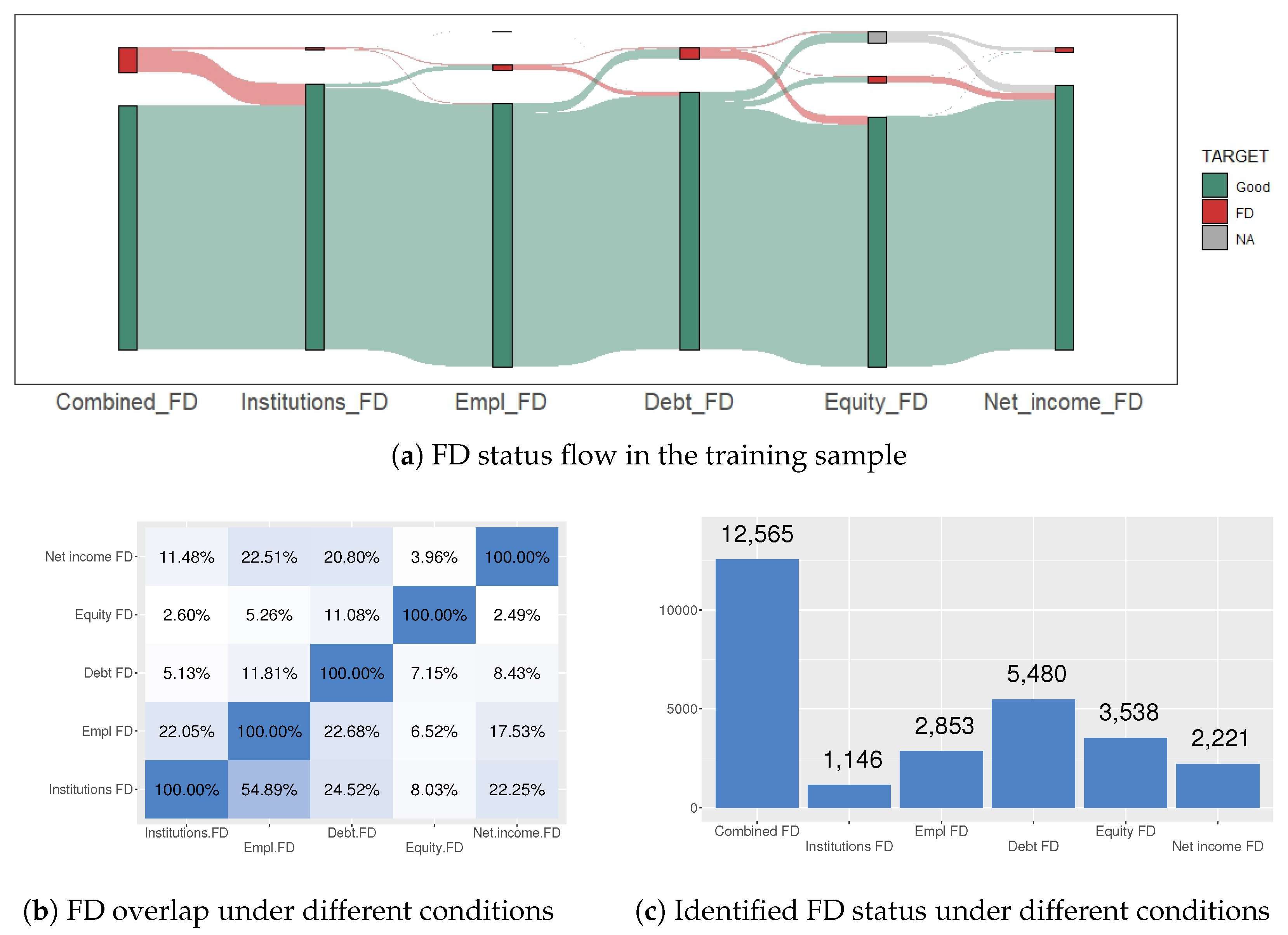
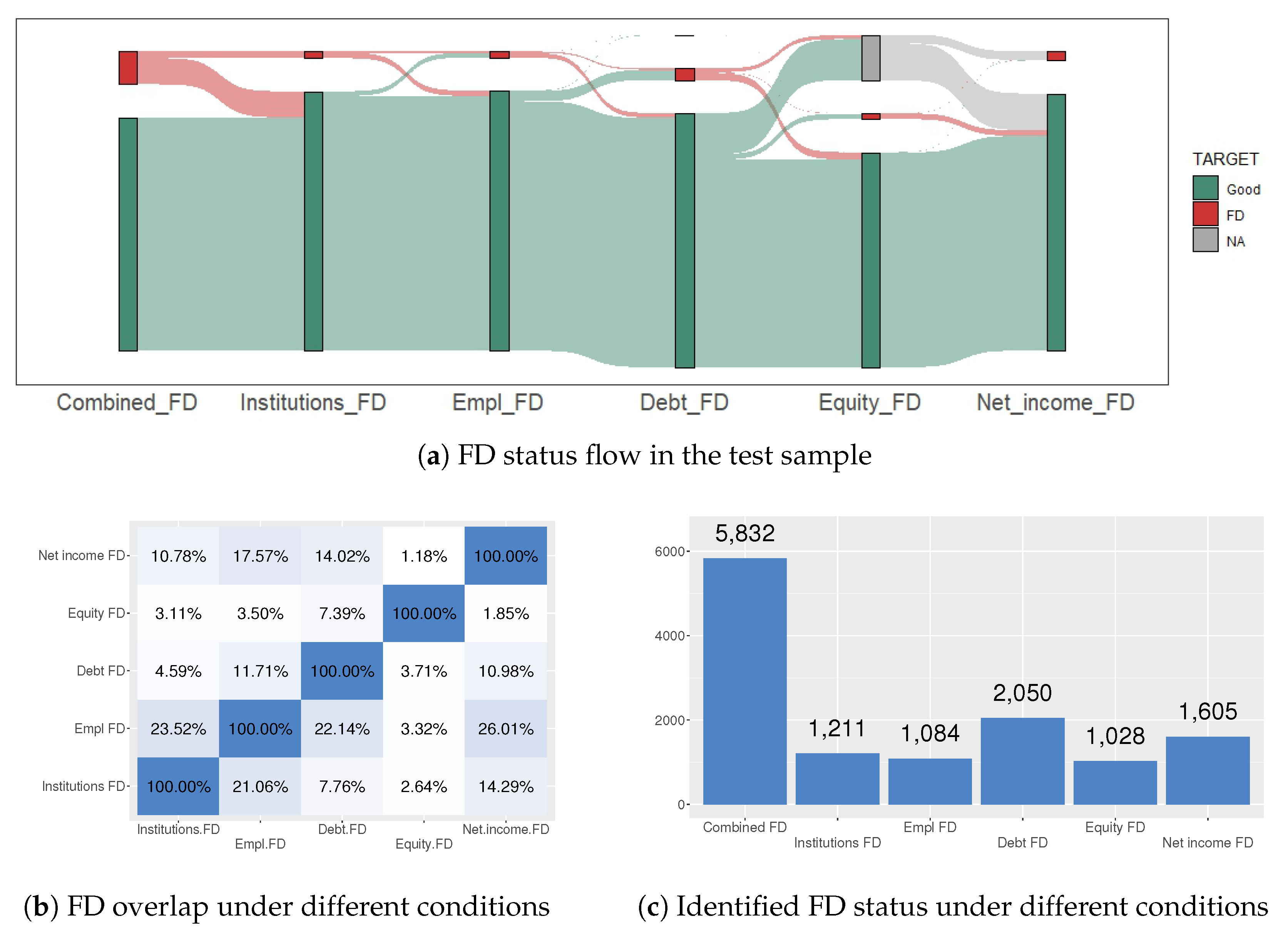
All of these definitions of financial distress conditions are presented in Section 4.1. They are connected by the “OR” operator for final financial distress determination. The distribution of the financial distress condition in the training and test sample is presented in Figure 2 and Figure 3. Comparing Figure 2a and Figure 3a, it is noticeable that the NA values of Equity_FD are higher in the test dataset. The reasoning behind this is as follows:

• The enterprise has not submitted a financial statement on time. The financial statement was downloaded on 12 July 2023. According to the law, enterprises must submit the FS 6 months after the end of the period;
• The enterprise submitted a misleading financial statement (see Section 4.1.4);
• The enterprise’s FS period is different.

From Figure 2b and Figure 3b, it is observed that there are not many overlaps between different financial distress conditions. A more intense color in Figure 2b and Figure 3b indicates greater overlap. The y axis of these graphs represents the overlap of one FD status over another FD status, i.e., Figure 2b Institutions FD overlap EMPL FD by 54.89%, but EMPL FD overlaps institutions FD by only 22.05%. FD statuses are affected by the difference in the number of cases (see Figure 2c Institutions FD—1146, Empl FD—2853). Also, it can be noticed that Debt_FD determines the highest number of FD conditions for enterprises (see Figure 2c and Figure 3c).

3.3. Features

The data used in this research can be divided into nine different categories, depending on the provider of the data or the information (see

Table 4. Characteristics of the features.

	Data Category	No.	Subcategory	Abbreviation	No.	Periodicity
						Stable	Depending on Event	Annually	Quarter	Monthly
1	Board, top management, shareholders	55	Main	MNG	21		✓
			Previous management history	Bad_MNG	34		✓
2	Financial statements	160	Records	FS	72			✓
			Ratios	FS_R	84			✓
			Register capital change	CPTL	4		✓
3	Legal events	13	Lawsuit	LawS	8		✓
			Seized property	SzPr	5		✓
4	Macroeconomics indicators	247	Monthly	Macro_M	177			✓		✓
			Quarterly	Macro_Q	70			✓	✓
5	Sector’s	126	Nace code	Nace	17	✓
			State data agency information provider	SEC	25			✓
			Statistics from analyzed enterprises *	SEC_R	84			✓
6	State social insurance	398	Debt	SSI_D	248			✓		✓
			Employees	SSI_E	150			✓		✓
7	State tax inspectorate	5	-	STI	5			✓
8	Other	16	Address	Other	2		✓
			Age		1		✓
			History (Institution_FD)		5		✓
			Name		2		✓
			Size		1	✓
			Legal form	Lform	5	✓
Total:		1020

✓ applicable for a data category features; *—the same set of features as financial statement ratios, but are aggregated using mean metrics for NACE code.

). For example, three data source providers are combined in the sector’s category: (1) sector type, identified by the NACE category; (2) information on sector profitability, competitiveness, etc. from the Lithuanian Statistics Department; (3) sectoral indicators calculated by combining financial statement data and NACE types. The number of features shows how many features fall under this category. The data frequency is divided into three categories:

• Stable—information is constant, e.g., legal status, types of sectors;
• Depending on an event—changes when the event occurs, the number of courts, the number of changes of directors, the time elapsed since the last event, etc.;
• Periodic data (annual, quarterly, monthly)—information is updated at the indicated periodicity, e.g., financial reports, macro indicators, and the number of employees.

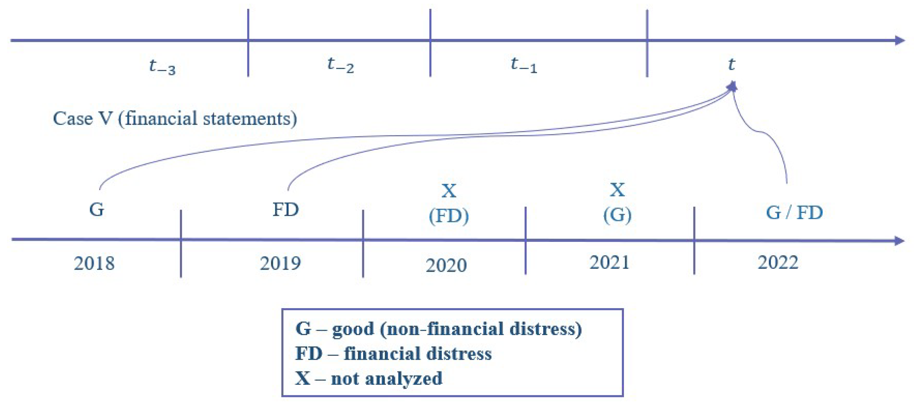
Periodic data correspond to time series data. Each period interval was treated as a separate feature. For example, from the balance sheet the feature “Total assets” (see Appendix C) is presented annually, therefore, the features of “total assets” are analyzed separately for the periods $t_1$, and $t_2$. The same condition was applied to the monthly data: the number of employees had been collected 36 times (i.e., monthly data for three years) along with various change statistics. The methodology’s concept is based on demonstrating AI’s ability to select important attributes without human intervention. Surprisingly, the conducted experiment revealed that the company’s debt in period $M_2$ is more significant than in period $M_1$.

All categorical features have been transformed into binary features by expanding the feature space. In the final dataset, each enterprise is described by 1016 features for each analyzed year.

4. Methodology

The aim of this research is to analyze the balancing technique’s influence on identifying financial distress. For this reason, various class balancing techniques were implemented in combination with different feature selection and machine learning methods. Hence, the focus of this research is to answer these questions:

RQ1:

What is the difference between machine learning model performances for different financial distress conditions?

RQ2:

How does the use of different feature selection techniques affect the results? Do selected features have the same patterns?

RQ3:

Which strategy is more effective for determining the size of features: an experimental or rule-based approach?

RQ4:

Which method of class balancing is the most effective for identifying financial distress?

RQ5:

Which machine learning model performs better in identifying financial distress?

The proposed framework for identifying financial distress is presented in Figure 4.

The first step deals with identifying primary conditions: expansion of class definition (see Section 4.1) and preparation of the final feature space (see Section 4.2). After creating the final dataset, the data are split into training and test samples. Cross-validation is not performed in order to obtain the classification evaluation results on the most relevant data and to provide market participants with current information about enterprises’ financial distress position. Hence, the test dataset uses the newest data and the training dataset uses data from 2018 to 2021. The ratio of the total data to the training and test samples is about 75:25.

The second step is data normalization. Normalization is a critical step in developing classification models with equal feature scales, i.e., it is performed to limit the dominance of specific features. The normalization process begins with the normalization of the training dataset, and then these normalization characteristics (identified by 2* arrow in Figure 4) are saved and used for normalizing the test dataset.

For the latest period data (test data), normalization is based on the features’ characteristics from previous years. Min–max normalization is used to scale the variables between zero and one [153]:

$$x_j^{\prime }=\frac{x_j-x_{j_{min}}}{x_{j_{max}}-x_{j_{min}}};$$

(2)

where $x_j$ is an original value of the j feature; $x_j^{\prime }$—the transformed value of the feature j; $x_{j_{min}}$ and $x_{j_{max}}$ are, respectively, the minimum and maximum values of a feature.

After normalization, all missing values (NA) are replaced by the smallest value—zero.

The third and fourth steps are related to the selection of important features and the identification of an optimal feature set. Firstly, feature selection techniques (see Section 4.3) rank the feature set in decreasing order of importance. The feature set is then narrowed down based on the chosen strategy: the experimental max number or the rule-based strategy (see Section 4.4).

The fifth step is either balancing or sampling the data. In this research, several oversampling, undersampling, and hybrid sampling techniques were used to give a better representation of the minority class instances (see Section 4.5). In addition, the non-balanced training dataset is also included in the comparison.

The sixth step is model training. Supervised machine learning classification methods, which are specified in Section 4.6, were used for identifying financial distress.

The seventh and eighth steps show the results after the classification and evaluation of the test data. The evaluation metrics are described in Section 4.7.

4.1. Class Definition Conditions

4.1.1. Financial Distress Identification from the Authoritative Institutions Perspective

The class being determined by the authorities is the worst-case of a financial distress scenario, as the chances for the enterprise to stop the bankruptcy or liquidation processes and recover are very little. Three authoritative institutions were analyzed as the main providers of information for identifying Institution’s financial distress:

• Registry center;
• State tax inspection;
• Courts.

Institutional financial distress class definition includes the following:

• A bankruptcy case that is filed against the enterprise;
• The enterprise’s status in the register center being changed to going bankrupt, bankrupt, under restructuring, under liquidation, etc.;
• The enterprise having made announcements to the register center about bankruptcy, liquidation, restructuring, insolvency, etc.;
• The enterprise being included in the State tax inspectorate’s lists of:

  (a)

  Companies temporarily exempt from submitting declarations to the STI,

  (b)

  Companies that have declared temporary inactivity to the STI;

  (c)

  Companies for which the STI has submitted a proposal to the State Register for deregistration following Article 2.70 of the Civil Code.

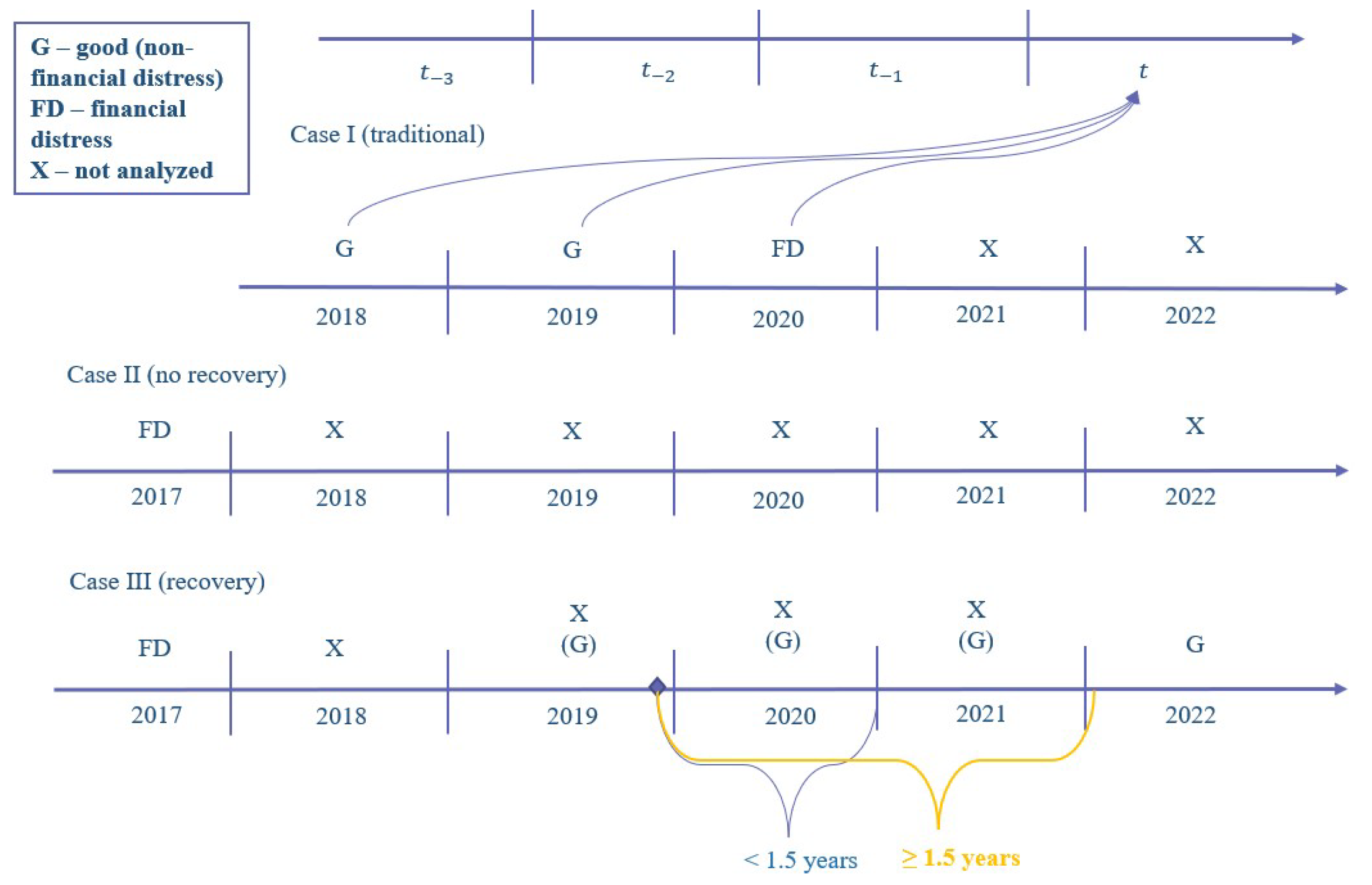
The enterprise may experience several of these events at once. For instance, an enterprise might be listed in the STI (State Tax Inspectorate) while its status in the registry center is marked as ‘under liquidation’. In such case, the earliest date of the first incident is determined. The enterprise is then placed in the FD category and is not further examined until the recovery criterion is satisfied. Notwithstanding, the likelihood of an enterprise satisfying the recovery criterion, i.e., the enterprise’s status changing to no legal proceedings in the registry center, is low. This is classified as the beginning of a recovery event, and after the 1.5 year recovery period is over, the enterprise is then included back into the sample (see Figure 5).

4.1.2. Financial Distress Identification from the Drop in Employees’ Perspective

A sudden decrease in the number of employees in an enterprise’s activities indicates an unclear internal situation of the enterprise, which can be linked to financial distress. However, the identification has to be made after the seasonality condition is checked.

For finding stable seasonal patterns, the Kruskal–Wallis test is used [154]. The selected significance level is $0.05$, i.e., smaller p-values suggest that there are indications of seasonality in the time series. Seasonality is analyzed for enterprises that meet these conditions:

• The minimum number of employees has to be >0 during the t and $t_{-1}$ years;
• The mean of employees ($Emp{l}_m$ see Equation (1)) has to be >5 and <250 during the $t_{-1}$ year;
• Available information about employees in an enterprise is ≥26 months.

Every year, the seasonality of enterprises is checked. If the enterprise meets the requirements to qualify as a seasonal one, it is included in the list of seasonal enterprises.

It is evident that due to the time series being too short, determining the seasonality of some enterprises will not be possible. For this reason, sectors with the greatest seasonality (according to NACE: A, B, C, F, G, I, see Appendix A) had been identified and were considered, just like the Agr enterprises, as seasonal enterprises.

Employee’s financial distress class definition includes:

• If the minimum number of employees is >0 in period t:
  • The maximum number is >5 in period t, and the enterprise is not indicated as seasonal, i.e., is not included in the seasonal enterprise’s sample or is not assigned to seasonal legal status or enterprise sectors. If all conditions are satisfied, then the following indicators are calculated:

    $${\mathit{Empl}}_{\mathit{12}}\mathit{M}\mathit{change}=\frac{{\mathit{Empl}}_{12}-M}{M},$$

    (3)

    $${\mathit{Empl}}_{\mathit{12}}\mathit{Max}\mathit{change}=\frac{{\mathit{Empl}}_{12}-Max}{Max},$$

    (4)

    $${\mathit{Empl}}_{\mathit{12}}{\mathit{Empl}}_{\mathit{1}}\mathit{change}=\frac{{\mathit{Empl}}_{12}-{\mathit{Empl}}_1}{{\mathit{Empl}}_1};$$

    (5)

    where ${Empl}_{12}$—the number of employees on December 31 of the period t; M—median of the number of employees during the year, max—max number of employees during the period t, ${Empl}_1$—the number of employees on January 31 of the period t.
    After calculating the indicators, the change is analyzed, and if the change meets at least one of the conditions specified in

    Table 5. Conditions for financial distress from drop in employees perspective.

    Size		Rule for FD		${\mathit{t}}_{-1}$	$\sum {\mathit{t}}_{-1}+{\mathit{t}}_{-2}$
    50–250	3	${Empl}_{12}Mchange$	<	−0.5	−0.7
    		${Empl}_{12}Maxchange$	<	−0.5	−0.7
    		${Empl}_{12}{Empl}_{1}change$	<	−0.5	−0.7
    10–50	2	${Empl}_{12}Mchange$	<	−0.5	−0.7
    		${Empl}_{12}Maxchange$	<	−0.7	−0.7
    		${Empl}_{12}{Empl}_{1}change$	<	−0.7	−0.7
    <10 (Max > 5, prevMax > 5)	1	${Empl}_{12}Mchange$	<	−0.7	−0.9
    		${Empl}_{12}Maxchange$	<	−0.8	−0.9
    		${Empl}_{12}{Empl}_{1}change$	<	−0.8	−0.9

    , the enterprise is identified as being in financial distress.
• If the minimum number of employees = 0 in period t:

  (a)

  For ≥3 months:

  • Legal status is PLL or PbLL;

  (b)

  For <3 months:

  • The maximum number of employees is >5, the minimum number of employees is >0 in period $t_{-1}$, and the enterprise is not indicated as seasonal. The conditions of seasonality and financial distress are the same as in the first case.

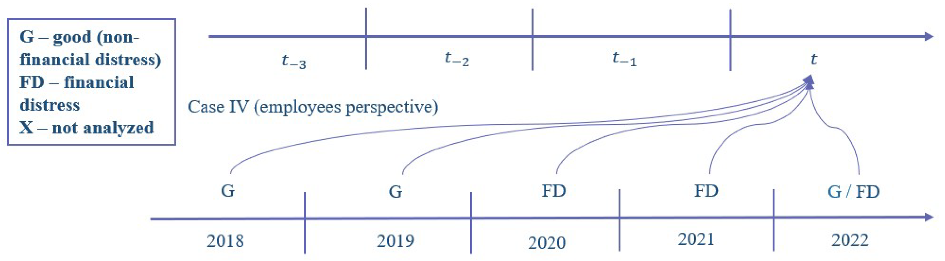
These conditions do not encompass all micro-enterprises due to the insufficient number of employees required for seasonality determination and implementation of drop in employees perspective. Moreover, the recovery criterion is not implemented, which allows the enterprises to have FD status for two consecutive years (see Figure 6).

4.1.3. Financial Distress Identification from a Debt Perspective

The enterprises having overdue financial obligations is a key indicator of financial distress. However, the availability of this kind of data is limited. The Lithuanian government gave information to the State Social Insurance about how many people work for the enterprises without paying social insurance taxes. The debt information was not used for identifying financial distress. Since the size of the debt depends on the size of the enterprise, a debt of 10,000 EUR is large for one enterprise, but small for another. For this reason, we created a flexible indicator—$SocialInsuranceBurden$, see Equation (6):

$$\mathit{Social}\mathit{Insurance}\mathit{Burden}=\frac{\mathit{Max}\mathit{Debt}}{\mathit{Min}\mathit{Pay}};$$

(6)

where the indicator $\mathit{Social}\mathit{Insurance}\mathit{Burden}$ shows how deep in debt an enterprise is if it pays minimal month’s salary (MMS) to its employees; $MaxDebt$—max debt during the period t, and $MinPay$ calculation is shown in Equation (7):

$$\mathit{MinPay}={\mathit{Empl}}_m\times \mathit{MMS}\times 0.2;$$

(7)

where $MinPay$—indicates a minimal amount of payment, i.e., cases where employees did not work for a full month and have been paid more than the minimum wage are not analyzed. $Emp{l}_m$—mean number of employees in period t; $MMS$—the minimal month’s salary in period t (see

Table 6. Minimal month’s salary (brutto), in EUR [155].

Year	2015	2016	2017	2018	2019	2020	2021	2022	2023
Minimal months salary (Brutto), MMS	300	350	380	400	555	607	642	730	840

). The indicator 0.2 is a minimum state social insurance tax payment from brutto salary for the employee.

Debt financial distress class definition is:

• If ${\mathit{Empl}}_m$≠ 0:
  • $\mathit{Social}\mathit{Insurance}\mathit{Burden}$ ≥ 3 and Debt is overdue for ≥90 days.
• If ${\mathit{Empl}}_m$= 0:

  (a)

  Legal status is PLL or PbLL:

  • Debt is overdue for >15 days.

  (b)

  Legal status is Agr, Ind, or SCom:

  • $\mathit{Social}\mathit{Insurance}\mathit{Burden}\mathit{II}$ ≥ 3 and debt is overdue for ≥90 days.

The second condition is noteworthy due to the legal nature of the Agr, Ind, or SCom enterprises, i.e., enterprises, which provide opportunities for employment without the need for socially insured workers. Therefore, a correction in the $\mathit{Social}\mathit{Insurance}\mathit{Burden}$ formula is made by removing the zero indicator (${\mathit{Empl}}_m$):

$$\mathit{Social}\mathit{Insurance}\mathit{Burden}\mathit{II}=\frac{\mathit{Max}\mathit{Debt}}{(\mathit{MMS}\times 0.2)}.$$

(8)

However, Agr, Ind, or SCom enterprises can operate without employees, and the possibility of debt to this institution becomes questionable. Nevertheless, the debt overdue is smaller, for PLL or PbLL enterprises due to the unclear situation with these enterprises.

The recovery criterion is not implemented, as in the drop in employee’s perspective (see Figure 6) which allows the enterprise to have an FD status for two consecutive years.

4.1.4. Financial Distress Identification from Financial Statements Perspective

The identification of financial distress from financial statements is widely analyzed in the literature (see Table 1). As a result, two indicators were chosen for recognizing financial distress:

• Equity $<0$ (negative) for period t;
• Net income $<0$ (loss) for t and $t_{-1}$ consecutive periods.

To clarify, the main reasons behind choosing these indicators are as follows:

• NA (not available data) values being present in financial statements. The deeper a subcategory in the statement is, the fewer areas are filled, e.g., interest expense is filled only 12–33% depending on the analyzed year. The completion level of a financial statement is given in Appendix B. Also, NA values double, if a ratio is present;
• unsuitability for SME analysis, e.g., if total liabilities divided by Total Equity is chosen as an indicator, almost all FD enterprises would be present, due to the main financing coming from equity.
• Overlaying results, i.e., net loss overlays 100% of the negative earnings results and ∼96% of the operating profit results.

Misstatements are eliminated before the financial statements are analyzed. For a financial statement to be considered for this analysis, it has to have:

• Balance sheet:

  (a)

  Total assets = long-term assets + short-term assets

  (b)

  Total equity and liabilities = equity (net worth) + amounts payable and liabilities + grants and subsidies

  (c)

  Amounts payable and liabilities = long-term amounts payable and liabilities + short-term amounts payable and liabilities

  (d)

  Total assets ≥ 0;

  (e)

  All statements in balance sheet ≠ 0.

• Income statement:

  (a)

  All statements in the income statement ≠ 0;

  (b)

  All profits (gross, operating, net) ≠ 0;

  (c)

  All costs ≠ NA or opposite sign. Here, ‘opposite sign’ implies that costs which increase profit do not decrease it.

In the analysis, only enterprises, which have provided at least one financial statement from the last two years, are included. For this reason, NA values are treated as FD conditions of previous years, see

Table 7. Equity and net income condition.

Equity
No.	${\mathit{t}}_{-\mathbf{2}}$	${\mathit{t}}_{-\mathbf{1}}$	t	Status
1	NA	NA	Not analyzed
2	1	NA	Not analyzed
3	0/1/NA	1	Not analyzed
4	0/1/NA	0	1	FD
5	0/1/NA	0	0/NA	Good
Net Income
No.	${\mathit{t}}_{-\mathbf{2}}$	${\mathit{t}}_{-\mathbf{1}}$	t	Status
1	NA/1	NA/1	Not analyzed
2	0	NA/1	NA/1	FD
3	0	NA/1	0	Good
4	0/1/NA	0	0/1/NA	Good

NA—not available data; FD—Financial distress.

.

The financial statements of enterprises are not analyzed until their recovery period has passed. The criterion of recovery for financial statements is shown in Figure 7.

4.2. Feature Set Preparation

The list of all features is presented in different tables sorted by data category (see Table 4) and shown in Appendix C. However, not all features are included in the analysis due to not having variance. These features are crossed out in Appendix A and eliminated from the study.

The selection of financial ratios for inclusion in the analyses has been based on the fulfillment of financial statements (see Appendix B), with a minimum of >50% of filled values (not NA) being considered. These values are not filled due to differences in FS templates for enterprises, which depend on the size, legal form, etc., of the enterprise. Moreover, the percentiles’ method has been used for all financial ratios, i.e., all observations that lie outside the interval formed by the 2.5 and 97.5 percentiles are considered as potential outliers [156] and their values are changed to NA (not available data). However, this implementation has not been sufficient for some features, which is why the percentiles’ method was repeated. In Appendix D, the statistics of financial ratios before and after using the percentiles’ method are presented.

For all these time-related features, like the time after the director change or the last lawsuit, the Equation (9) is applied, after calculating the feature duration in days:

$$\widehat{{\mathit{Time}}_{\mathit{d}}}=\frac{1}{{\mathit{Time}}_{\mathit{d}}};$$

(9)

where ${\mathit{Time}}_{\mathit{d}}$ is the number of days that have passed after the event, and $\widehat{{\mathit{Time}}_{\mathit{d}}}$ is a derivative attribute, which indicates a greater significance the closer it is to the present. If ${\mathit{Time}}_{\mathit{d}}$ is equal to 0, then $\widehat{{\mathit{Time}}_{\mathit{d}}}$ is equal to 1.

4.3. Feature Selection Methods

The incorporation of new features into the model is related to detecting early warning signals and creating more precise models. However, the expansion of the feature space has a negative impact that occurs through data sparsity, multiple testing, multicollinearity, and overfitting problems [9]. To overcome these difficulties, different dimensionality reduction techniques are used. In this study (based on previous research), several embedded techniques have been used that belong to the feature selection approach. This approach determines a narrow subset of informative features from the original wide range of data [157] by removing irrelevant, redundant, or noisy features. Also, the embedded technique uses machine learning models for feature selection.

• LASSO (least absolute shrinkage and selection operator) is a method that combines feature selection and regularization. This method thins out the feature space by reducing some regression coefficients to zero [158]. The features that are left (non-zero) are then prioritized by the absolute value of LASSO regression coefficients. LASSO defines a limited group of features, which makes the interpretation of a model more accurate and is used for further classification [24].
• The random forest (RF) employs two methods for prioritizing features, both of which involve aspects of feature cost and the ability to differentiate [159].

  (a)

  MDA (mean decreasing accuracy) or permutation importance prioritizes features depending on the model accuracy, i.e., measuring the importance of features before and after the permutation in the OOB (out of bags) accuracy [160,161].

  (b)

  MDG (mean decreasing gini) or MDI (mean decreasing impurity) prioritizes features after estimating the sum over the number of splits (through all trees) that include the feature, corresponding to the number of samples it separates [160,161].

• XGBoost (extreme gradient boosting machine) uses the gain metrics to prioritize each feature. The greater the XGBoost gain, the greater the feature’s involvement is in the decision making regarding outcomes [162,163].
• $\mathit{Voted}\_\mathit{imp}$ (Voted importance) prioritizes features depending on the combined rank from all the feature selection methods.

4.4. Number of Features

Despite the lack of information on the requirement for a maximum feature set for efficient model creation, the researchers focus on implementing the dimensionality reduction techniques. Hence, this research creates several new research directions to fill this gap.

• Experimental max number strategy narrows the prioritized feature set to an experimentally chosen number of features from a lower-dimensional space, specifically, $k\in \{15,30,50,100\}$.
• Rule-based strategy takes the most effective feature’s value, which is given by the embedded model, then splits it in half ($v_h$), and all the features valued > $v_h$ go to a final dataset. Also, this strategy could be called half of the highest value strategy. According to this strategy, in this research, the k value for LASSO is 5, RF-MDA—36, RF-MDG—20, XGBoost—4. Since this strategy for the $\mathit{Voted}\_\mathit{imp}$ has to include 321 features, it was modified by only including overlapping features with ≥0.9 combined ranking score, then $k=8$.

4.5. Class Balancing Techniques

Let $Y=\{y_1,y_2,\dots ,y_n\}$ denote the class labels, where n is the number of enterprises and $y_i\in C=\{0,1\},i=1,\dots ,n$ belongs to one of the two classes: $c_1$—non-financial distress (majority class) or $c_2$—financial distress (minority class). Each enterprise is defined by a number of features $x_{ij}$, $j=1,\dots ,d$. The balancing ratio ($\mathit{BR}$) of the training dataset T is:

$$\mathit{BR}=\frac{T_{c_{\mathit{min}}}}{T_{c_{\mathit{maj}}}}=\frac{T_{c_{\mathit{2}}}}{T_{c_{\mathit{1}}}}.$$

(10)

The ratio’s values range from 0 to 1, the smaller the number, then the more difficult the task will be for a learner [135]. Financial distress and bankruptcy are rare events for the enterprises, and hence, the $BR$ for these events is from 0.01 to 0.001 [124]. This lack of data from the minority class makes the majority classes dominate evaluation metrics, i.e., the learner can attain 99 percent accuracy without classifying rare examples [164]. For this reason, it is better to use AUC, Gini, G-mean, Recall, and Precision metrics [9].

The problem of class imbalance can be solved by using three different approaches: data-level, algorithm-level, and hybrid. The data-level approach involves modifying the data to ensure a more equitable distribution of classes. In contrast, the algorithm-level approach makes adjustments to the learner’s bias, prioritizing minority classes in the learning process. The hybrid approach combines data-level and algorithm-level approaches. In this research, the data-level approach, which separates the sampling and the classifier training processes, is used. To be more precise, the following techniques were employed:

• Oversampling—a technique, used to increase the amount of data. It modifies the original dataset by replacing or creating new data samples (generally the minority ones) [165]. The advantages of this technique include the enhancement of learner performance and a more precise representation of the two classes.

  (a)

  SMOTE (synthetic minority oversampling technique) is an oversampling technique that generates synthetic examples from the minority class to achieve a balanced dataset distribution [131,166]. SMOTE employs the k-NN method for the identification of the k-nearest neighbors of the minority class, and then generates synthetic examples by interpolating the reference sample with a randomly selected object from its neighborhood [167]. The SMOTE-generated samples are linear combinations between two similar samples from the minority class ($x_{i.}$ and $x_{i.}^R$) and are defined as [166,168]:

  $$x_{i.}^{*}=x_{i.}+u(x_{i.}^R-x_{i.});$$

  (11)

  with $x_{i.}^{*}$ generated synthetic samples; $0\le$$\mathit{u}$$\le 1$; $x_{i.}^R$ is selected at random from the 5 nearest neighbors (minority class) of $x_{i.}$.

  (b)

  SMOTE-NC (smote-nominal, continuous) is an enhancement of the SMOTE method, that generates data in a continuous or nominal way, by employing the modified-Euclidean distances as in Equation (12), depending on the feature type [169]

  $$\Delta (x_{i.},x_{i.}^R)=\sqrt{\sum _{j_{\mathit{cont}}=1}^{d_{\mathit{cont}}}{(x_{i{j}_{\mathit{cont}}}-x_{i{j}_{\mathit{cont}}}^R)}^2+\sum _{j_{\mathit{nom}}=1}^{d_{\mathit{nom}}}{\mathit{Med}}_{j_{\mathit{nom}}}^2};$$

  (12)

  in which $\Delta (x_{i.},x_{i.}^R)$ is the distance between these observations; $d_{cont}$ and $d_{nom}$ are the number of continuous and nominal features, respectively; ${\mathit{Med}}_{j_{nom}}$ is the median value derived from the standard deviations of nominal features within the minority class [170,171,172]. If the features are continuous, $x_{ijcont}^{*}$ is calculated according to Equation (11). Otherwise, for nominal features, the median value is determined based on the majority voting of the k-nearest neighbors vector, with the category, that appears most frequently, chosen as the value for the new observation [170].

  (c)

  ADASYN (adaptive synthetic sampling approach) was proposed by He et al. [173] and was based on the SMOTE algorithm [174]. However, the disparities arise in the selection of density distribution for the automatic generation of sample sizes for minority classes [173]. The ADASYN algorithm generates minority-class samples in areas that are more difficult to learn [174]. It also determines how many synthetic samples are required for every minority example to be created, based on how many of its majority class nearest neighbors are involved. The proportion of the majority nearest neighbors has a direct impact on the quantity of synthetic samples generated for the minority class.

  However, the “noise” sample detection is not included in this algorithm. Thus, near-borderline sample generation could lead to the creation of an unrealistic minority space for the learner [174].

  (d)

  GAN (generative adversarial networks) is an adversarial modeling framework of two multi-layer perceptron models: a generator (G) and a discriminator (D) [175]. The G task is the generation of a synthetic data sample, which would be identical to real data [149]. However, the G task is judged by a discriminator (D), which is a binary classifier for the recognition of the real data from generated [148]. GAN has shown success in complex high-dimensional distributions of real-world data, such as image generation, image-to-image synthesis, image super-resolution, etc. [147,148,149]. Nevertheless, the potential of GAN can be found when solving class imbalance problems, as it can generate samples of the minority class [147]. It is known that, in the best-case scenario, the training process continues until D can no longer recognize real samples from generated samples, i.e., the global optimal solution is obtained [148]. However, it can be stopped after reaching a specified number of iterations or at the local minimum [147]. The GAN optimization problem is defined as follows:

  $$\underset{G}{min}\underset{D}{max}V(D,G)={\mathbb{E}}_{x\sim P_{\mathit{T}}{\mathit{c}}_{\mathit{2}}}\left[\mathit{log}D\left(x\right)\right]+{\mathbb{E}}_{\tilde{z}\sim P_{\mathit{T}}{\mathit{c}}_{\mathit{2}}\left(\tilde{z}\right)}\left[\mathit{log}(1-D\left(G\left(\tilde{z}\right)\right))\right];$$

  (13)

  where $P_{T_{c_2}}$, $P_G$, and $P_{\tilde{Z}}\left(\tilde{z}\right)$ are real training minority class samples, generated samples, and noise variable distribution, respectively; $G\left(\tilde{z}\right)$ is a function of mapping noise to a data space, and $D\left(x\right)$ shows the probability that the sample x is real data rather than a generated sample. The GAN is trained to maximize $D\left(x\right)$ and to minimize $D\left(G\left(\tilde{z}\right)\right)$ [148,175].

  (e)

  ROSE (random over-sampling examples) is based on using a smoothed bootstrap approach for generating new synthetic data for the classes (minority and majority) [176,177]. This oversampling technique begins with estimating the multivariate probability density function (PDF) for each class. Then, this estimation is used to draw samples [178]. Essentially, an observation belonging to one of the two classes is extracted from the training dataset and a new sample $(x^{*},y^{*})$ is created in its neighborhood. The neighborhood’s shape is defined by the contour sets of K, with its width controlled by $H_c$ [165].

• Undersampling—a data cleaning technique, which reduces the original dataset by removing samples (usually belonging to the majority class) from it [165]. Decision surface cleaning, class overlap reduction, and ‘noisy’ sample removal are some of the main advantages of this technique [179].

  (a)

  The K-mean algorithm determines the cluster centroid by measuring the separation between each data point in the cluster, which is then used to cluster data [180]. Then, the algorithm detects and removes samples, that are in narrow, borderline, and noisy areas from the majority class until the intended balance is reached [181].

  (b)

  Nearmiss (removes points near other classes) is an undersampling technique, that eliminates the samples from the majority class by implementing the k-NN algorithm. The selected majority class samples for removal are near to some samples of minority classes [165,182]. Nonetheless, this method removes the points from the majority class, which have the smallest mean distance to the k-nearest points from the minority class.

  (c)

  RUS (random undersampling) is a non-heuristic technique that seeks to produce a balanced instance set by randomly removing instances of the majority class in order to balance the distribution of classes [165].

• The hybrid sampling technique combines both oversampling and undersampling techniques.

  (a)

  SMOTE-ENN combines the SMOTE and edited nearest neighbor (ENN) techniques and is assigned to the hybrid sampling technique group [183]. SMOTE is an oversampling technique, which generates synthetic samples for the minority class. However, these generated samples could bring more noise to the dataset [184] or complicate the work of the classifier by creating boundary samples [185]. In order to overcome these disadvantages, the ENN technique is used, which removes samples from both classes [186]. The ENN algorithm can be described as a data cleaning method, which may remove any sample whose class label is different from the class of two or more of its closest neighbors [183].

  (b)

  SMOTE-TL is a hybrid technique, which combines SMOTE and the Tomek links (TL) techniques. The TL technique is used for the same reasons as ENN—to reduce SMOTE disadvantages. Unlike ENN, TL analyzes only two samples that are the nearest neighbors and belong to different classes [187]. If $x_{i_{c_1}.}$ and $x_{i_{c_2}.}$ are the samples of the majority and minority classes, then a Tomek link is a distance between the pair $(x_{i_{c_1}.},x_{i_{c_2}.})$ [188,189], assuming no other class $x_{i_{knn}}$ that fulfills the requirements listed below:

  $$\Delta (x_{i_{c_1}.},x_{i_{\mathit{knn}}.})<\Delta (x_{i_{c_1}.},x_{i_{c_2}.})\mathit{or}\Delta (x_{i_{c_2}.},x_{i_{\mathit{knn}}.})<\Delta (x_{i_{c_1}.},x_{i_{c_2}.}).$$

  (14)

  Here, samples from both classes are removed instead of only samples from the majority class. A Tomek link is a good indicator for noisy or borderline connection [187], which can also be applied for post-processing, data cleaning [189].

For balancing techniques, whose nominal feature values had been changed to continuous, the feature-converting rule (Equation (15)) was applied to the nominal value. For example, the binary feature’s $L\_form.PLL$ values, after applying the SMOTE technique, have changed to values $\{0,0.333,\dots ,0.99,1\}$; thus, the feature converting rule has been used

$$x_{i{j}_{\mathit{nom}}}=\left\{\begin{array}{cc}1,\hfill & x_{i{j}_{\mathit{nom}}}\ge 0.5\hfill \\ 0,\hfill & x_{i{j}_{\mathit{nom}}}<0.5\hfill \end{array}\right..$$

(15)

4.6. Machine Learning Methods

The field of study known as machine learning (ML) pertains to the study of computer algorithms, specifically the automated learning process that is facilitated through experience [190].

For financial distress classification, several supervised machine learning methods were used, and the selection process was influenced by previous research [9].

• Boosting is a powerful ensemble learning technique that transforms a group of learners from weak learners into strong learners by minimizing training errors [9]. The training process goes sequentially by reweighting and modifying current weights based on how accurately the previous learners predicted these samples [191]. In this study, categorical boosting (CatBoost) and extreme gradient boosting machine (XGBoost) techniques were implemented.

  (a)

  CatBoost (categorical boosting) is a new gradient boosting technique that implements ordered boosting into processing of categorical features [192]. Gradient boosting has a prediction shift problem, which ordered boosting solves. CatBoost is a modification of gradient boosting that avoids target leakage, i.e., ordered boosting splits the training dataset so that the model could be trained on one subset of data, while residuals could be calculated on another. Moreover, the processing of categorical features replaces the original, categorical variables with one or more numerical values, which reduces the number of steps in data preprocessing [193].

  (b)

  XGBoost (extreme gradient boosting machine) is a fast learning algorithm that combines gradient descent and tree ensemble learning to solve classification and regression problems [140]. Its main idea is to make the target function as minimal as possible while employing the gradient descent method to produce new trees based on all previous trees [194].

• DT (decision tree) extracts decision rules from a dataset and represents it in a tree-like structure for solving classification and regression problems [195]. The DT algorithm CART (classification and regression tree), which uses the Gini coefficient for the internal/decision node splitting, was implemented. The decision tree is a nonparametric method, and hence a small change in the data can develop a new tree [9].
• LDA (linear discriminant analysis) is a classification technique that searches for a linear combination of features, which would make a separation of the classes in the most efficient way, i.e., it maximizes the variance between classes and minimizes the variance within a class [196,197].
• LG (logistic regression) is a statistical method used for modeling relationships between dependent and independent features. Moreover, the logistic function is used to model binary ($C=\{0,1\}$) dependent variables [9,198]. Based on our previous research, the assumption of multicollinearity is fulfilled for the LR method, i.e., features from the balanced dataset, that are highly correlated with other features, are removed.
• NB (naive Bayes) is based on the statistical Bayes theorem. It describes the probability of a given class label, based on features that might be related to a particular class label [158].
• Neuron networks is a group of ML methods that represent information processing in the mathematical manner of biological systems [199].

  (a)

  ANN (artificial neural network) is a computational model interconnected with a layered structure that contains input, output, and one or more hidden layer [200]. The multi-layer perception (MLP) is a popular type of ANN, where a feed-forward manner is used to place nodes and layers. Several processing layers causes the nonlinear associations between inputs and outputs to be created [94]. The hidden structure of the neuron network has been marked I–III, which indicates the hidden layers between input and dense layers. After each layer (except a dense one), a drop-out layer is implemented which is excluded from the calculation of the hidden structure.

  (b)

  CNN (convolutional neural network) is a deep learning architecture, which has a direct learning process from data. It works well for a large number of labeled data. The CNN architecture consists of convolution, pooling, and fully connected layers. These layers are used for automatic and adoptive learning of features for the classification tasks [9]. The hidden structure is indicated the same as in ANN. However, this indication is only used for conv_1d and flat layers; input, drop out, max-pooling, and the dense layer are not included in the calculation of the structure of the hidden layers.

  (c)

  ELM (extreme learning machine) is a training algorithm for single hidden layer feedforward neural networks. A normal distribution is used to assign weights between the input and hidden layers, while the pseudo-inverse technique is used to learn the weights between the hidden and output layers [201]. Moreover, the main benefits of ELM are fast learning speed, ease of implementation, and less human intervention when compared to the standard neural networks [202]. ELM was implemented with numeric values of $\{100,150,200,300\}$ for the hidden neurons.

• Random forest (RF) is an ensemble technique that involves creating multiple decision trees using various subsets of samples from the original dataset. Each tree in the RF is generated from a bootstrap sample of the data. Numerous individual trees are created, which have a low correlation with one another. In addition, the majority of these trees’ votes decide the class’s label [123,203].
• SVM (support vector machine) seeks to separate the classes by identifying the optimal decision boundary in a high-dimensional feature space. The possibilities of decision boundaries depend on the used SVM kernel function [9,204]. For example, a linear kernel makes the assumption that the relationship between the features and the class is linear. Hence, it tries to separate the classes in a linear manner. More complex decision boundaries (curves, circles, etc.) can be found using non-linear kernels, such as polynomial or radial basis functions. All these types of SVM kernel functions have been used in this research.
• WMA (weighted majority algorithm) is a compound algorithm formed from a pool of known algorithms [205,206]. In this research, several combinations of WMA (see

  Table 8. Combinations of the weighted majority algorithm.

  	ANN2	CatBoost	XGBoost	DT	LG	NB	RF	SVM (Linear)
  WMA_3.1		✓	✓				✓
  WMA_3.2	✓			✓			✓
  WMA_3.3	✓	✓					✓
  WMA_3.4		✓			✓		✓
  WMA_3.5			✓		✓		✓
  WMA_3.6					✓	✓	✓
  WMA_5.1	✓	✓	✓	✓	✓		✓
  WMA_5.2	✓		✓	✓	✓		✓
  WMA_5.3	✓			✓	✓		✓	✓
  WMA_5.4	✓	✓		✓	✓		✓
  WMA_5.5	✓	✓			✓	✓	✓
  WMA_5.6		✓	✓	✓	✓		✓
  WMA_7.1	✓	✓	✓	✓	✓	✓	✓
  WMA_7.2	✓	✓	✓	✓	✓		✓	✓

  ✓ inclusion of an ML model into the weighted majority algorithm.

  ) were analyzed, but in all of these combinations, the algorithms are equally weighted in the voting process.

4.7. Evaluation Metrics

Evaluation metrics are determined based on the confusion matrix (see

Table 9. Confusion matrix [165].

		Predicted Class
		Non-Financial Distress	Financial Distress	Total
Actual class	Non-financial distress	$\mathit{TP}$	$\mathit{FN}$	$\mathit{POS}$
	Financial distress	$\mathit{FP}$	$\mathit{TN}$	$\mathit{NEG}$
	Total	$\mathit{PPOS}$	$\mathit{PNEG}$	$\mathit{N}$

). In this research, non-financial distress enterprises are assigned to the positive class ($c_1=\left\{0\right\}$) and financial distress enterprises are assigned to the negative class ($c_2=\left\{1\right\}$). In Table 9, $\mathit{TP}$ denotes the number of true positives, $\mathit{TN}$ is the number of true negatives, $\mathit{FP}$ is the number of false positives, $\mathit{FN}$ is the number of false negatives, $POS$ is the number of actual positives, $\mathit{PPOS}$ is the number of predicted positives, $\mathit{NEG}$ is the number of actual negatives, $\mathit{PNEG}$ is the number of predicted negatives, and N is the number of all instances [165].

The most commonly used evaluation metrics, that are provided in Equations (16)–(23), were chosen for this research [9]. Moreover, higher values indicate a better performance for all these evaluation metrics.

• Precision—the ratio of true positives ($\mathit{TP}$) to predicted positives ($\mathit{PPOS}$)

  $$\mathit{Precision}=\frac{\mathit{TP}}{\mathit{TP}+\mathit{FP}}.$$

  (16)
• Recall—the ratio of the true positives ($\mathit{TP}$) to actual positives ($\mathit{POS}$), also known as sensitivity or $\mathit{TPR}$ (true positive ratio)

  $$\mathit{Recall}=\frac{\mathit{TP}}{\mathit{TP}+\mathit{FN}}.$$

  (17)
• Specificity—the ratio of the true negatives ($TN$) to the actual negatives ($\mathit{NEG}$). Also known as $\mathit{TNR}$ (true negative ratio)

  $$\mathit{Specificity}=\frac{\mathit{TN}}{\mathit{TN}+\mathit{FP}}.$$

  (18)
• The area under the ROC curve (AUC)—a measure of how well a model can distinguish between two classes and is expressed as follows:

  $$\mathit{AUC}={\int }_0^1\left(\mathit{TPR}\right)d\left(\mathit{FPR}\right);$$

  (19)

  where false positive ratio $\mathit{FPR}$ = 1—specificity.
• The $Gini$ is a metric that indicates the model’s discriminatory power. It is used as an alternative to AUC and usually used more often in the context of bankruptcy prediction. Moreover, the simple expression of $\mathit{Gini}$ is:

  $$\mathit{Gini}=2\mathit{AUC}-1.$$

  (20)
• Accuracy ($ACC$)—the proportion of correctly classified instances

  $$\mathit{ACC}=\frac{\mathit{TP}+\mathit{TN}}{\mathit{TP}+\mathit{TN}+\mathit{FP}+\mathit{FN}}.$$

  (21)
• F-$score$ is the harmonic mean of precision and recall, where the most common value of $\beta$ is 1. Therefore, the estimate is often called $F1$ or $F1$-$score$

  $$\mathit{F}-\mathit{score}=\frac{(1+{\beta }^2)\mathit{Precision}·\mathit{Recall}}{{\beta }^2·\mathit{Precision}+\mathit{Recall}}.$$

  (22)
• The G-$mean$ is a geometric mean of the true positive rate and the true negative rate.

  $$\mathit{G}-\mathit{mean}=\sqrt{\mathit{TPR}·\mathit{TNR}}.$$

  (23)

5. Results

This experimental study examines the impact of diverse financial distress class definitions (determinations) in conjunction with balancing techniques to construct an efficient financial distress detection model. The experimental results involve five feature selection techniques, using 5 different number of feature set combinations, 10 different balancing techniques, 11 different machine learning models, and 14 different weighted majority algorithm combinations. In total, 9428 experiments have been conducted for the test dataset. The test sample had been separated from the training sample and included the last year’s (2022) data. Additionally, balancing techniques for the training sample have not been applied (see Figure 4). Thus, providing relevance to the current SMEs financial distress situation. To evaluate the efficiency of the model, the effectiveness criteria have been implemented. These criteria require that half of the good classification from both classes is present. However, as the test dataset is unbalanced, these halves are ≥$2900$ financial distress cases, and ≥20,600 non-financial distress cases. If this criterion is not filled, the outcome of the experiment is not further analyzed. This requirement has reduced the number of total experiments by approximately $25\%$, resulting in $7101$ experiments.

Table 10. Performance results ranged by AUC score metrics for financial distress detection (Combined FD).

	Feature Method	No.	No. Category	Balancing Technique	Balancing Category	Method Specific	Accuracy	AUC	F-1	G-Mean	Gini	Precision	Recall	Specificity
1	XGBoost	30	Exp	Nearmiss	Under	WMA_3.1	0.8908	0.8559	0.9354	0.8547	0.7118	0.9710	0.9023	0.8095
2	XGBoost	50	Exp	RUS	Under	WMA_3.1	0.8641	0.8559	0.9179	0.8558	0.7118	0.9753	0.8668	0.8450
3	XGBoost	50	Exp	RUS	Under	WMA_5.1	0.8640	0.8559	0.9178	0.8558	0.7117	0.9753	0.8667	0.8450
4	XGBoost	30	Exp	RUS	Under	WMA_3.1	0.8716	0.8555	0.9229	0.8552	0.7109	0.9739	0.8769	0.8340
5	XGBoost	30	Exp	RUS	Under	WMA_5.1	0.8809	0.8551	0.9290	0.8544	0.7102	0.9723	0.8894	0.8208
6	XGBoost	50	Exp	Nearmiss	Under	WMA_3.1	0.8822	0.8538	0.9299	0.8529	0.7076	0.9717	0.8916	0.8160
7	Voted_imp	100	Exp	RUS	Under	WMA_7.1	0.8937	0.8535	0.9373	0.8518	0.7070	0.9698	0.9069	0.8001
8	XGBoost	100	Exp	RUS	Under	WMA_5.1	0.8606	0.8534	0.9156	0.8534	0.7069	0.9751	0.8629	0.8440
9	XGBoost	100	Exp	RUS	Under	WMA_3.1	0.8607	0.8534	0.9156	0.8534	0.7068	0.9751	0.8631	0.8438
10	XGBoost	30	Exp	RUS	Under	CatBoost	0.8792	0.8532	0.9279	0.8525	0.7063	0.9719	0.8877	0.8186
11	Voted_imp	100	Exp	RUS	Under	WMA_7.2	0.8862	0.8527	0.9325	0.8515	0.7054	0.9707	0.8972	0.8081
12	RFMDG	100	Exp	RUS	Under	WMA_7.1	0.8992	0.8524	0.9408	0.8501	0.7048	0.9686	0.9146	0.7901
13	XGBoost	30	Exp	RUS	Under	WMA_3.3	0.8612	0.8522	0.9160	0.8521	0.7044	0.9745	0.8642	0.8402
14	LASSO	100	Exp	Nearmiss	Under	WMA_3.3	0.8732	0.8521	0.9240	0.8516	0.7042	0.9725	0.8801	0.8241
15	RFMDA	100	Exp	RUS	Under	WMA_7.1	0.8931	0.8521	0.9369	0.8503	0.7041	0.9694	0.9066	0.7975
16	XGBoost	30	Exp	RUS	Under	WMA_3.4	0.8888	0.8519	0.9342	0.8505	0.7038	0.9700	0.9010	0.8028
17	LASSO	100	Exp	RUS	Under	WMA_3.3	0.8642	0.8518	0.9180	0.8517	0.7036	0.9739	0.8682	0.8354
18	LASSO	100	Exp	RUS	Under	WMA_5.1	0.8747	0.8518	0.9251	0.8513	0.7036	0.9722	0.8823	0.8213
19	LASSO	100	Exp	Nearmiss	Under	WMA_5.1	0.8836	0.8518	0.9308	0.8507	0.7036	0.9708	0.8941	0.8095
20	XGBoost	50	Exp	Nearmiss	Under	CatBoost	0.8892	0.8517	0.9345	0.8503	0.7035	0.9699	0.9015	0.8020
21	XGBoost	30	Exp	RUS	Under	WMA_3.5	0.8891	0.8516	0.9344	0.8501	0.7032	0.9699	0.9014	0.8018
22	LASSO	100	Exp	RUS	Under	CatBoost	0.8606	0.8516	0.9156	0.8515	0.7032	0.9744	0.8635	0.8397
23	LASSO	100	Exp	RUS	Under	WMA_3.4	0.8733	0.8515	0.9241	0.8510	0.7029	0.9723	0.8806	0.8224
24	RFMDG	100	Exp	RUS	Under	WMA_7.2	0.8910	0.8515	0.9356	0.8498	0.7029	0.9695	0.9040	0.7989
25	RFMDG	100	Exp	RUS	Under	WMA_5.5	0.8710	0.8514	0.9226	0.8510	0.7027	0.9726	0.8775	0.8253
26	XGBoost	30	Exp	Nearmiss	Under	CatBoost	0.8937	0.8512	0.9374	0.8494	0.7025	0.9690	0.9077	0.7948
27	RFMDG	100	Exp	RUS	Under	WMA_5.6	0.8509	0.8511	0.9091	0.8511	0.7023	0.9759	0.8508	0.8515
28	XGBoost	50	Exp	RUS	Under	CatBoost	0.8632	0.8510	0.9174	0.8509	0.7021	0.9738	0.8672	0.8349
29	LASSO	100	Exp	Nearmiss	Under	WMA_3.4	0.8899	0.8510	0.9349	0.8494	0.7019	0.9695	0.9027	0.7992
30	XGBoost	100	Exp	RUS	Under	CatBoost	0.8616	0.8508	0.9164	0.8507	0.7016	0.9740	0.8652	0.8364
31	XGBoost	30	Exp	RUS	Under	WMA_5.6	0.8799	0.8507	0.9285	0.8498	0.7014	0.9710	0.8895	0.8119
32	LASSO	100	Exp	Nearmiss	Under	WMA_5.6	0.8838	0.8506	0.9310	0.8495	0.7013	0.9703	0.8947	0.8066
33	LASSO	100	Exp	Nearmiss	Under	CatBoost	0.8787	0.8505	0.9277	0.8497	0.7010	0.9711	0.8880	0.8129
34	LASSO	100	Exp	Nearmiss	Under	WMA_3.1	0.8744	0.8505	0.9249	0.8499	0.7009	0.9718	0.8823	0.8186
35	RFMDG	100	Exp	RUS	Under	WMA_5.1	0.8497	0.8504	0.9083	0.8504	0.7008	0.9759	0.8495	0.8513

The best scores of evaluation metrics are in bold.

shows the best models based on the AUC metric. This metric was selected as the main metric for analysis since it can balance expressions for both classes. Also, additional evaluation metrics are provided to make this research more easily comparable with others. The best AUC score ($0.8559$) is achieved using XGBoost feature selection technique with experimental max number strategy, Nearmiss, or RUS undersampling methods, and WMA_3.1 weighted majority algorithm (i.e., with CatBoost, XGBoost, and RF have equal voting weights). Moreover, Catboost has achieved the best result ($0.8539$), when analyzing algorithms individually. In the methodology part, five research questions were raised. The answers to each research question are presented in separate research parts, which are set out below.

5.1. Financial Distress Conditions Analysis

Experiments held in this section have been designed to explore the potential of different financial distress conditions by answering the first research question: what is the difference between the machine learning model performances for different financial distress conditions? The combined FD definition aggregates several conditions with the “OR” operator, i.e., Institutions FD, Empl FD, Debt FD, Equity FD, and Net income FD (see Section 4.1). All methods have been trained on the combined FD definition. However, the results of the test dataset have been checked for each condition separately. Moreover, for each condition, the effectiveness criteria were recalculated depending on each condition class size. If the conditions have missing values (NA), they are removed from the analysis of a particular test dataset; this was relevant for Debt FD and Equity FD conditions.

Table 11. Number of experiments before and after the application of the effectiveness criteria.

Name	Before	After	Eff, %
Combined FD	9428	7101	75.32%
Institutions FD	9428	6608	70.09%
Empl FD	9428	2930	31.08%
Debt FD	9428	7981	84.65%
Equity FD	9428	1918	20.34%
Net income FD	9428	7396	78.45%

represents the percentage of effective experiments left after implementing the effectiveness criteria. Debt FD and Net income FD had the highest number of effective experiments, in contrast to Equity FD and Empl FD.

Table 12. The analysis of performance results for financial distress conditions.

Feature Method	No.	No. Category	Balancing Technique	Balancing Category	Method Specific	Accuracy	AUC	F-1	G-Mean	Gini	Precision	Recall	Specificity
Combined FD
RFMDA	100	Exp	GAN	Over	WMA_3.3	0.9520	0.8341	0.9731	0.8192	0.6681	0.9560	0.9908	0.6773
XGBoost	30	Exp	Nearmiss	Under	WMA_3.1	0.8908	0.8559	0.9354	0.8547	0.7118	0.9710	0.9023	0.8095
XGBoost	50	Exp	RUS	Under	WMA_3.1	0.8641	0.8559	0.9179	0.8558	0.7118	0.9753	0.8668	0.8450
RFMDG	20	Rul	K-mean	Under	WMA_3.3	0.5795	0.7318	0.6881	0.7033	0.4637	0.9828	0.5294	0.9343
XGBoost	15	Exp	NO	NO	WMA_5.3	0.9369	0.7560	0.9651	0.7168	0.5120	0.9357	0.9964	0.5156
RFMDG	20	Rul	K-mean	Under	WMA_5.6	0.5722	0.7279	0.6809	0.6978	0.4558	0.9826	0.5209	0.9348
Institutions FD
RFMDA	15	Exp	NO	NO	SVM (linear)	0.9936	0.8801	0.9967	0.8720	0.7603	0.9937	0.9997	0.7605
RFMDA	15	Exp	ROSE	Over	DT	0.9799	0.8988	0.9896	0.8947	0.7976	0.9950	0.9843	0.8134
XGBoost	15	Exp	K-mean	Under	WMA_3.3	0.5962	0.7654	0.7391	0.7444	0.5309	0.9975	0.5870	0.9438
Voted_imp	100	Exp	K-mean	Under	WMA_5.5	0.5176	0.7287	0.6715	0.6939	0.4574	0.9975	0.5061	0.9513
Empl FD
LASSO	100	Exp	ADASYN	Over	XGBoost	0.8747	0.6940	0.9323	0.6677	0.3880	0.9870	0.8834	0.5046
RFMDG	100	Exp	RUS	Under	CatBoost	0.7416	0.7254	0.8488	0.7252	0.4508	0.9908	0.7423	0.7085
Voted_imp	100	Exp	Nearmiss	Under	CatBoost	0.6610	0.7117	0.7915	0.7097	0.4233	0.9917	0.6586	0.7648
Voted_imp	100	Exp	K-mean	Under	WMA_5.5	0.5086	0.6553	0.6660	0.6370	0.3105	0.9911	0.5015	0.8090
Debt FD
XGBoost	4	Rul	NO	NO	ANN2	0.9850	0.8981	0.9922	0.8931	0.7962	0.9910	0.9933	0.8029
XGBoost	4	Rul	ROSE	Over	WMA_3.6	0.9559	0.9493	0.9765	0.9492	0.8985	0.9972	0.9566	0.9420
LASSO	50	Exp	ADASYN	Over	ANN1	0.6665	0.8208	0.7889	0.8032	0.6415	0.9993	0.6518	0.9898
Voted_imp	100	Exp	ROSE	Over	XGBoost	0.9783	0.7629	0.9888	0.7254	0.5257	0.9788	0.9989	0.5268
Voted_imp	50	Exp	K-mean	Under	WMA_3.4	0.5646	0.7677	0.7054	0.7347	0.5354	0.9992	0.5451	0.9902
Equity FD
XGBoost	100	Exp	Nearmiss	Under	WMA_3.5	0.8698	0.6833	0.9294	0.6543	0.3665	0.9845	0.8801	0.4864
XGBoost	4	Rul	ADASYN	Over	ANN2	0.6571	0.7539	0.7873	0.7469	0.5077	0.9941	0.6517	0.8560
XGBoost	4	Rul	ADASYN	Over	WMA_3.3	0.7333	0.7504	0.8424	0.7502	0.5008	0.9915	0.7323	0.7685
RFMDG	20	Rul	K-mean	Under	WMA_5.6	0.5217	0.7071	0.6755	0.6794	0.4141	0.9949	0.5114	0.9027
Net income FD
RFMDG	50	Exp	GAN	Over	SVM (linear)	0.9965	0.9964	0.9982	0.9964	0.9928	0.9999	0.9965	0.9963
XGBoost	4	Rul	RUS	Under	WMA_5.4	0.8196	0.9066	0.8970	0.9018	0.8132	1	0.8132	1

The best scores of evaluation metrics are in bold.

presents the best performance results (in bold) of each evaluation metric separately, according to financial distress conditions. Institutions FD is the worst-case financial distress scenario as it includes bankruptcy, liquidation and similar statuses (see Section 4.1). Therefore, the Institution’s FD is comparable to the task of identifying bankruptcy. According to the literature review, the most frequently attained AUC score ranges from $0.82$ to $0.95$. However, the highest AUC ($0.9994$) score was found in the research [6]. This raises additional questions about data sparsity and method validation. In our research, for the Institutions FD condition, a typical AUC score of $0.8988$ was achieved. This was obtained using the RFMDA feature selection technique, experimental max number strategy, ROSE oversampling methods, and the DT method.

However, the most difficult FD classification task appeared to be for the condition of Empl FD, due to checking for seasonality and the distinct requirements for enterprises of different legal statuses. The Kruskal–Wallis test, which is a non-parametric test for detecting seasonality based on ranks, was used to check for seasonality in Empl FD. It should be noted that the auto-ARIMA algorithm was used for removing any autocorrelation or noise from the data before applying the Kruskal–Wallis test.

The result of the non-parametric Kruskal–Wallis test is more accurate compared to the results from the Dickey–Fuller test, the Mann–Kendall trend Test, the Friedman rank test, etc. However, due to the absence of annotated data, the efficiency of the method remains unknown. Also, the legal exceptions for the enterprises of different legal status make the Empl FD classification task very complicated. Therefore, it would be more appropriate to create separate models, e.g., SCom enterprises can function well without employees, while it is impossible for a PLL enterprise to not have employees. Nonetheless, our data indicate that some PLL enterprises still work without having employees, and some of them even exhibit seasonal trends.

In contrast, the task of classifying Debt FD had one of the best AUC scores ($0.9493$), which had been reached with only four features chosen by the XGBoost feature selection method. The high accuracy in Debt FD classification is attributed to implementing the ‘worst’ debt condition, i.e., debt overdue 90 days.

Based on the financial statements and the literature analysis, two FD conditions have been proposed: Equity FD and Net income FD. The Net income FD classification task exhibited the highest scores for each evaluation metric. The best results for the Net income FD were achieved with the GAN balancing technique and linear SVM, without distinguishing feature selection methods. When analyzing Table 7 from the perspective of a ML classification task, unfortunately, examples that satisfy the third condition are very rare. Therefore, the main task of the classifier is to separate the second and the third conditions in Net income FD. However, by balancing classes, additional FD events, i.e., more examples that satisfy the second condition, are created. Hence, the training dataset mainly consists of data that satisfy the second and the fourth conditions, which can be described as the rule-based method. For example, in the test sample, there are 116 examples that satisfy the third condition, which is only 7% of FD cases (1606).

Whilst the Equity FD separation task is very difficult, as identical equity conditions can result in FD and non-FD. Moreover, the data analysis has shown that negative equity (FD) is also possible for enterprises that showed millions of equity in financial statements a year ago. Nevertheless, the best AUC score ($0.7539$) was achieved with XGBoost feature selection technique, rule-based number strategy, ADASYN oversampling methods, and a neural network with two hidden layers.

5.2. Feature Selection

In this section, the second research question is analyzed: How does the use of different feature selection techniques affect the results? Do selected features have the same patterns?

The overlapping features between different feature selection techniques are presented in Figure 8a. Obviously, $\mathit{Voted}\_\mathit{imp}$ is the most overlapping technique of all methods. XGBoost and RFMDG follow next, despite measuring the importance differently. The LASSO method stands out the most because it has the least overlap with all the other techniques (except $\mathit{Voted}\_\mathit{imp}$). This study demonstrates that utilizing diverse techniques, distinct properties are selected, resulting in distinct sets of properties. This enables us to identify the optimal combination of methods for addressing the FD problem.

Figure 8b shows the comparison of FS technique usability for each data category (Table 4). Feature selection techniques were chosen mostly from FS, STI, SSI, and other data source categories. However, the best Combined FD score has been achieved with a set of 30 features obtained through XGBoost, which also included indicators from macroeconomics, board, top management, and shareholders data categories. In addition, Figure 8b shows that an increase in the number of feature sets, increases the similarity in data category distribution for different methods, except the LASSO technique.

5.3. Number of Feature Set Selection

This section presents the results of the strategy for determining the number of features by answering the third research question: which strategy is more effective for determining the size of features: an experimental or rule-based approach?

In Section 4.4, the experimental max number and rule-based strategies are described. For the latter, the k values are as follows: for LASSO—5, RF-MDA—36, RF-MDG—20, XGBoost—4. Whereas, for the experimental max number strategy, $k\in \{15,30,50,100\}$. Figure 9 shows the distribution of AUC scores across different feature selection strategies under various FD conditions. The outcomes depicted in this graph are remarkably similar, with a few noticeable gaps. Hence, a single strategy is not suitable for all feature selection methods. This thesis is confirmed by Figure 10 and Figure 11. The rule-based strategy is best suited for XGBoost, and RF-MDG methods (see Table 10 and Table 12 and Figure 10 and Figure 11). In addition, the result of XGBoost has shown that a high AUC score ($0.9493$) could even be achieved with four features. Two of these features are from FS and the other two are from SSI data categories (bold in Appendix C). However, this approach is not suitable for the LASSO technique. In this research, the LASSO method achieved the best scores when using the maximum number of features. However, in our previous research, the best results with LASSO were achieved using between 30 and 50 features. LASSO differs from other feature selection techniques, in that without seeding, there is a possibility of having different sets of features in each iteration.

5.4. Class Balancing Techniques

This section presents the results related to the fourth research question: which method of class balancing is the most effective for identifying financial distress?

Figure 12 and Figure 13 show the efficiency of using balancing techniques under different FD conditions. The ROSE technique stands out in these figures as it exhibited the lowest number of effective experiments across all FD conditions, while the remaining experiments failed to demonstrate a high AUC ranking (with the exception of Institutions FD). While GAN performed well in classifying the Net income FD, it failed to classify Equity FD and Empl FD conditions. Moreover, a non-balance case is marked as “NO” in the figures. Its unsuitability for difficult classification tasks (Equity FD, Empl FD) can be seen in the figures. Moreover, there is no noticeable distinction between the results attributed to the Smote family (SMOTE, ADASYN, SMOTE-NC, SMOTE-ENN, SMOTE-TL).

Figure 14 demonstrates the sparsity of the applied method in relation to the complexity of the classification task. For example, Debt FD and Net income FD have shown that the best classification results could be achieved with different balancing techniques (favoring oversampling methods). But as the task becomes more difficult, data cleaning becomes increasingly important. Hence, undersampling or oversampling techniques, which focus on generating samples in areas that are more difficult to learn (such as ADASYN), start to provide better results. When comparing undersampling methods, the RUS and Nearmiss methods have shown the best results in performance. In future research, using the Nearmiss method is suggested, in order to avoid the randomness effect.

5.5. Machine Learning Methods

In this section, the last research question is analyzed: which machine learning model performs better in financial distress identification?

The experiments employed 11 distinct machine learning models, with their respective modifications (a total of 21), and 12 weighted majority algorithms (WMAs). The most time-consuming experiment, i.e., linear SVM method (XGBoost (100), with no balancing technique), lasted up to 4.67 days. Comparing the results for SVM, for this task, the linear SVM model is more accurate than Polynomial SVM or Radial SVM. In addition, Figure 15 shows that LG, naive Bayes, and WMA_7 group methods are rarely used in harder classification tasks (Empl FD and Equity FD). The highest AUC score among these methods was achieved using WMA_7, whereas the best score with single classifiers was $0.677$. Moreover, the highest AUC score for the net income condition was $0.9891$. The best AUC scores of the model groups for the Combined FD are presented in Figure 16. The CatBoost, XGBoost, RF, and LG performed the best as single classifiers. Of course, better results were achieved by making combinations for WMAs. Furthermore, the most successful results were obtained with WMA using three model ensembles. Figure 17 illustrates that, in almost all scenarios, the best-averaged outcomes are achieved by WMA_3.1—an ensemble with equal voting weights assigned to CatBoost, XGBoost, and RF algorithms.

6. Discussion

This section provides a discussion on the main aspects of financial distress identification analysis: financial distress conditions and the effectiveness of imbalance techniques in creating future research guidelines.

Researchers agree that financial distress is a situation in an enterprise where it has difficulties fulfilling its financial obligations. Nevertheless, a lack of consensus regarding the indication of a class’s financial distress condition remains. Table 1 presents 29 potential class indicators for such classification. However, when viewed from the perspective of SMEs, this number decreases to 14. Moreover, factors such as unavailable data, unsuitability, and overlapping suggestions further diminish this count. Consequently, this study incorporates two financial distress conditions identified through literature analysis (equity and negative income), one analogy of bankruptcy (Institutions FD), and proposes two new conditions (a sudden decrease in Employees (Empl) and Debt). The performance of Compound FD and the worst-case scenario (Institution FD) has been found to be similar to what is reported in the literature analysis. The best results typically exhibit AUC fluctuations between 80 and 90%. The results of this research indicate that at least 8 out of 10 SMEs will be accurately assessed for the FD condition if an equal proportion of FD and non-FD cases is present. Machine learning algorithms struggled to accurately classify negative equity, but performed well with negative net income. The financial statements revealed instances where enterprises with significant equity in one year experienced subsequent periods of negative equity, raising concerns about the reliability of financial reporting. Conversely, the predictability of negative net income was attributed to its requirement to persist over two consecutive years, resulting in few transitions from negative to positive income, resembling a rule-based model’s analysis. The available government data allowed the suggestion of two new FD condition directions. Assessing the FD condition from the number of employees was challenging due to the diverse legal obligations of various enterprise types. Additionally, annotating the data and employing various ML algorithms could enhance the detection of seasonality, improving the recognition of financial distress from Empl. Conversely, identifying financial distress from a debt perspective showed excellent results. The strong association between financial distress and the level of an enterprise debt suggests that the inclusion of enterprise debt information could broaden this concept. In the research, a worst-case debt scenario was initially implemented, but it had been designed to be adaptable. This adaptability in model creation accommodates varying levels of risk aversion among beneficiaries.

As demonstrated by the diverse financial distress (FD) conditions, classification tasks can be categorized into easier and more challenging ones, contingent upon the available dataset. It is noted that, for easier classification tasks, high-efficiency results can be achieved with most class imbalance techniques. Furthermore, a variation in the results shown in the literature is evident, with achieved AUC results ranging from 71.4% [150] to 99.98% [108]. Of course, various types of datasets are analyzed, including private data, stock market data, datasets from different data providers, as well as data from SMEs, etc. This diversity in dataset types contributes to the variability observed in the results. In this research, the GAN, as a financial distress class sample generator technique, was explored and compared in this research with other data-level approach techniques. The samples produced by the GAN technique did not display notable differences compared to other oversampling methods. Nevertheless, the GAN technique proved particularly effective in simpler classification tasks, especially in classifying the negative Net income FD condition. Conversely, the hybrid sampling techniques did not exhibit clear superiority over other methods across diverse FD conditions. Consequently, different sampling procedures produced better performance outcomes for different financial distress conditions. It is still unclear whether the oversampling or undersampling approach should be preferred for identifying financial distress. For further analysis, we suggest incorporating oversampling techniques such as ADASYN, SMOTE, ROSE, and GAN, along with undersampling techniques like RUS and Nearmiss.

Finally, the aim of this research is to provide insight into financial distress detection. We created a methodology framework that is easy to adopt for analyzing your own financial distress datasets. The crafted methodology covers and analyzes each aspect separately, starting from identifying financial distress problems, focusing on the use of different datasets, preparing data for machine learning algorithms (including dimensionality reduction, addressing class imbalance, and classification), and selecting evaluation metrics. Further analysis in this area should continue to expand and delve deeper into the analyzed areas. We suggest focusing on recognizing financial distress from the debt condition parameter, as empirical evidence suggests promising outcomes. The inclusion of many macro and sector indicators expanded the dimensionality of the dataset but did not show promising results. The area of using embedded methods with an optimal set of parameters requires further in-depth investigation. While, in this study, we incorporated data-level approach techniques to address data imbalance, further research could explore algorithm-level techniques. What concerns benchmark ML models, authors should incorporate LR, DT, RF, XGBoost, CatBoost, and SVM (linear) in the analysis, as they often show promising results. When these methods are not applied for comparison, it can be difficult to evaluate different articles. To ensure comparability of the results, it is essential to include the AUC among different metrics.

7. Conclusions

This research presents the methodology for advanced financial distress detection using artificial intelligence. The analyzed methodology includes different combinations of financial distress conditions, reduction in the high-dimensional feature space, involving class balancing techniques, and implementing machine learning models. The comparison of previous financial distress studies and their reliance on SMEs offered several possible FD conditions. All recommendations from the researchers pertain to financial statement data. To ensure available and non-overlapping data, two of the proposed conditions were chosen: equity and net income. However, having access to the institution (status changes to bankruptcy, liquidation, etc.), debt, and employee data, we extended the FD condition with these formed conditions. Hence, Combined FD has been constructed from the Institutions FD, Empl FD, Debt FD, Equity FD, and Net income FD. Then, the research was expanded with dataset construction, including all available enterprise-characterizing features. This high-dimensional feature space has been reduced by using embedded feature selection techniques and several feature set determination strategies. The main focus of this research was the usage of balancing techniques. In the bankruptcy and FD topics, the most used techniques are SMOTE and its different modifications. Nevertheless, the expansion of our research has involved not only the inclusion of undersampling or hybrid techniques but also the implementation of GAN networks as a data oversampling technique. Moreover, 11 different machine learning methods (with their modifications, totaling 21) and 12 weighted majority algorithms were implemented.

This research used data from Lithuanian SMEs from 1 January 2015 to 30 December 2022 provided by LTD Baltfakta. Based on the methodology and available data, the best AUC score for Combined FD was 0.8559, which is achieved with the XGBoost feature selection technique, an experimental max number strategy, Nearmiss or RUS undersampling methods, and the WMA 3.1 weighted majority algorithm (i.e., with CatBoost, XGBoost, and RF have equal voting weights). The findings of the five research questions are presented in the following conclusions:

• Financial distress conditions results separated the FD conditions into the simpler and harder classification tasks. Moreover, these results uncovered which areas need adjustment in future research (Empl FD—seasonality, Net income FD—third condition). In addition, it has been shown that a good result can also be achieved with a four-variable model under the Debt FD condition.
• The different embedded feature selection methods revealed that, without $\mathit{Voted}\_\mathit{imp}$, the most overlaps occur using XGBoost and RFMDG techniques, while the LASSO technique has the least overlap. Moreover, the most commonly used data categories are FS, STI, SSI, and other.
• For determining feature set size two strategies were analyzed: the experimental max number and rule-based. The research results reveal that neither strategy works for all feature selection methods. The rule-based strategy is suitable for XGBoost and RF-MDG methods, but not suitable for LASSO or $\mathit{Voted}\_\mathit{imp}$.
• The research results on balancing techniques demonstrated their correlation with the complexity of the classification task. The simpler classification task does not pinpoint a single balancing technique; instead, several techniques showed satisfactory results. Meanwhile, as the classification condition becomes more challenging, the applicability of the balancing method diminishes, e.g., for financial distress, undersampling techniques begin to show better outcomes, and oversampling techniques also focus on generating samples in regions where learning is more challenging, which also proved to be effective.
• The analysis of machine learning methods revealed that the best-average performance had been achieved with WMA_3.1, which is an ensemble of equal voting weights of CatBoost, XGBoost, and RF algorithms. In addition, these algorithms with LG have shown the best performance as a single classifier.

The limitations associated with this research are as follows:

• Number of features. The experimental max number strategy involves only a small set of the possible features.
• Stability of the feature set. It was not examined whether the selected feature set would maintain its stability over time.
• Model specifications. Model parameter optimization was not performed. Instead, the results were compared using baseline models. Nevertheless, altering the quantity of features only caused minor variations in the neural network models’ output.

In further research, we plan to focus on improving FD conditions, especially the Empl FD seasonality condition. Moreover, we are interested in experimenting with feature set stability in different time frames and the applicability of research results in other markets.

References

- Sun, J.; Li, H.; Fujita, H.; Fu, B.; Ai, W. Class-imbalanced dynamic financial distress prediction based on Adaboost-SVM ensemble combined with SMOTE and time weighting. Inf. Fusion 2020, 54, 128–144. [Google Scholar] [CrossRef]
- Zoričák, M.; Gnip, P.; Drotár, P.; Gazda, V. Bankruptcy prediction for small- and medium-sized companies using severely imbalanced datasets. Econ. Model. 2020, 84, 165–176. [Google Scholar] [CrossRef]
- Shen, F.; Liu, Y.; Wang, R.; Zhou, W. A dynamic financial distress forecast model with multiple forecast results under unbalanced data environment. Knowl.-Based Syst. 2020, 192, 105365. [Google Scholar] [CrossRef]
- Faris, H.; Abukhurma, R.; Almanaseer, W.; Saadeh, M.; Mora, A.M.; Castillo, P.A.; Aljarah, I. Improving financial bankruptcy prediction in a highly imbalanced class distribution using oversampling and ensemble learning: A case from the Spanish market. Prog. Artif. Intell. 2020, 9, 31–53. [Google Scholar] [CrossRef]
- Gnip, P.; Drotár, P. Ensemble methods for strongly imbalanced data: Bankruptcy prediction. In Proceedings of the 2019 IEEE 17th International Symposium on Intelligent Systems and Informatics (SISY), Subotica, Serbia, 12–14 September 2019; pp. 155–160. [Google Scholar] [CrossRef]
- Papíková, L.; Papík, M. Effects of classification, feature selection, and resampling methods on bankruptcy prediction of small and medium-sized enterprises. Intell. Syst. Account. Financ. Manag. 2022, 29, 254–281. [Google Scholar] [CrossRef]
- Farooq, U.; Jibran Qamar, M.A.; Haque, A. A three-stage dynamic model of financial distress. Manag. Financ. 2018, 44, 1101–1116. [Google Scholar] [CrossRef]
- Yazdanfar, D.; Öhman, P. Financial distress determinants among SMEs: Empirical evidence from Sweden. J. Econ. Stud. 2020, 47, 547–560. [Google Scholar] [CrossRef]
- Kuizinienė, D.; Krilavičius, T.; Damaševičius, R.; Maskeliūnas, R. Systematic Review of Financial Distress Identification using Artificial Intelligence Methods. Appl. Artif. Intell. 2022, 36, 2138124. [Google Scholar] [CrossRef]
- Salehi, M.; Davoudi Pour, M. Bankruptcy prediction of listed companies on the Tehran Stock Exchange. Int. J. Law Manag. 2016, 58, 545–561. [Google Scholar] [CrossRef]
- Letizia, E.; Lillo, F. Corporate payments networks and credit risk rating. EPJ Data Sci. 2019, 8, 21. [Google Scholar] [CrossRef]
- Veganzones, D.; Severin, E. Corporate failure prediction models in the twenty-first century: A review. Eur. Bus. Rev. 2020, 33, 204–226. [Google Scholar] [CrossRef]
- du Jardin, P. Failure pattern-based ensembles applied to bankruptcy forecasting. Decis. Support Syst. 2018, 107, 64–77. [Google Scholar] [CrossRef]
- Du, X.; Li, W.; Ruan, S.; Li, L. CUS-heterogeneous ensemble-based financial distress prediction for imbalanced dataset with ensemble feature selection. Appl. Soft Comput. 2020, 97, 106758. [Google Scholar] [CrossRef]
- Gerged, A.M.; Yao, S.; Albitar, K. Board composition, ownership structure and financial distress: Insights from UK FTSE 350. Corp. Gov. Int. J. Bus. Soc. 2022, 23, 628–649. [Google Scholar] [CrossRef]
- Udin, S.; Khan, M.A.; Javid, A.Y. The effects of ownership structure on likelihood of financial distress: An empirical evidence. Corp. Gov. Int. J. Bus. Soc. 2017, 17, 589–612. [Google Scholar] [CrossRef]
- García, C.J.; Herrero, B. Female directors, capital structure, and financial distress. J. Bus. Res. 2021, 136, 592–601. [Google Scholar] [CrossRef]
- Boubaker, S.; Cellier, A.; Manita, R.; Saeed, A. Does corporate social responsibility reduce financial distress risk? Econ. Model. 2020, 91, 835–851. [Google Scholar] [CrossRef]
- Oware, K.M.; David Kweku Botchway, K. Exchange and moral capital of CSR disclosure and financial distress likelihood of family management firms: Evidence from India. Manag. Res. Rev. 2022, 46, 625–646. [Google Scholar] [CrossRef]
- Sareen, A.; Sharma, S. Assessing Financial Distress and Predicting Stock Prices of Automotive Sector: Robustness of Altman Z-score. Vis. J. Bus. Perspect. 2022, 26, 11–24. [Google Scholar] [CrossRef]
- Abdullah, M. The implication of machine learning for financial solvency prediction: An empirical analysis on public listed companies of Bangladesh. J. Asian Bus. Econ. Stud. 2021, 28, 303–320. [Google Scholar] [CrossRef]
- Kamalirezaei, H.; Rostamy, A.A.A.; Saeedi, A.; Zaghard, M.K.V. Corporate social responsibility and bankruptcy probability: Exploring the role of market competition, intellectual capital, and equity cost. J. Corp. Account. Financ. 2020, 31, 53–63. [Google Scholar] [CrossRef]
- Ali, S.; ur Rehman, R.; Yuan, W.; Ahmad, M.I.; Ali, R. Does foreign institutional ownership mediate the nexus between board diversity and the risk of financial distress? A case of an emerging economy of China. Eurasian Bus. Rev. 2021, 12, 553–581. [Google Scholar] [CrossRef]
- Zizi, Y.; Jamali-Alaoui, A.; El Goumi, B.; Oudgou, M.; El Moudden, A. An Optimal Model of Financial Distress Prediction: A Comparative Study between Neural Networks and Logistic Regression. Risks 2021, 9, 200. [Google Scholar] [CrossRef]
- Sewpersadh, N.S. An econometric analysis of financial distress determinants from an emerging economy governance perspective. Cogent Econ. Financ. 2022, 10, 1978706. [Google Scholar] [CrossRef]
- Doğan, S.; Koçak, D.; Atan, M. Financial Distress Prediction Using Support Vector Machines and Logistic Regression. In Advances in Econometrics, Operational Research, Data Science and Actuarial Studies: Techniques and Theories; Terzioğlu, M.K., Ed.; Contributions to Economics; Springer International Publishing: Cham, Switzerland, 2022; pp. 429–452. [Google Scholar] [CrossRef]
- Dumitrescu, A.; El Hefnawy, M.; Zakriya, M. Golden geese or black sheep: Are stakeholders the saviors or saboteurs of financial distress? Financ. Res. Lett. 2020, 37, 101371. [Google Scholar] [CrossRef]
- Li, C.; Lou, C.; Luo, D.; Xing, K. Chinese corporate distress prediction using LASSO: The role of earnings management. Int. Rev. Financ. Anal. 2021, 76, 101776. [Google Scholar] [CrossRef]
- Cheng, C.H.; Chan, C.P.; Sheu, Y.J. A novel purity-based k nearest neighbors imputation method and its application in financial distress prediction. Eng. Appl. Artif. Intell. 2019, 81, 283–299. [Google Scholar] [CrossRef]
- Pham Vo Ninh, B.; Do Thanh, T.; Vo Hong, D. Financial distress and bankruptcy prediction: An appropriate model for listed firms in Vietnam. Econ. Syst. 2018, 42, 616–624. [Google Scholar] [CrossRef]
- Hafeez, A.; Kar, S. Looking Beyond the Financial Numbers: The Relationship Between Macroeconomic Indicators and the Likelihood of Financial Distress. Glob. Bus. Rev. 2018, 22, 674–688. [Google Scholar] [CrossRef]
- Ugur, M.; Solomon, E.; Zeynalov, A. Leverage, competition and financial distress hazard: Implications for capital structure in the presence of agency costs. Econ. Model. 2022, 108, 105740. [Google Scholar] [CrossRef]
- Fernández-Gámez, M.A.; Soria, J.A.C.; Santos, J.A.C.; Alaminos, D. European country heterogeneity in financial distress prediction: An empirical analysis with macroeconomic and regulatory factors. Econ. Model. 2020, 88, 398–407. [Google Scholar] [CrossRef]
- Tran, K.L.; Le, H.A.; Nguyen, T.H.; Nguyen, D.T. Explainable Machine Learning for Financial Distress Prediction: Evidence from Vietnam. Data 2022, 7, 160. [Google Scholar] [CrossRef]
- Sehgal, S.; Mishra, R.K.; Jaisawal, A. A search for macroeconomic determinants of corporate financial distress. Indian Econ. Rev. 2021, 56, 435–461. [Google Scholar] [CrossRef]
- Quintiliani, A. Financial distress cost of Italian small and medium enterprises: A predictive and interpretative model. The J. Risk Financ. 2017, 18, 564–580. [Google Scholar] [CrossRef]
- Hernandez Tinoco, M.; Holmes, P.; Wilson, N. Polytomous response financial distress models: The role of accounting, market and macroeconomic variables. Int. Rev. Financ. Anal. 2018, 59, 276–289. [Google Scholar] [CrossRef]
- Freitas Cardoso, G.; Peixoto, F.M.; Barboza, F. Board structure and financial distress in Brazilian firms. Int. J. Manag. Financ. 2019, 15, 813–828. [Google Scholar] [CrossRef]
- Rezende, F.F.; da Silva Montezano, R.M.; de Oliveira, F.N.; de Jesus Lameira, V. Predicting financial distress in publicly-traded companies. Rev. Contab. Financ.—USP 2017, 28, 390–406. [Google Scholar] [CrossRef]
- Bravo-Urquiza, F.; Moreno-Ureba, E. Does compliance with corporate governance codes help to mitigate financial distress? Res. Int. Bus. Financ. 2021, 55, 101344. [Google Scholar] [CrossRef]
- Mousavi, M.M.; Ouenniche, J.; Tone, K. A dynamic performance evaluation of distress prediction models. J. Forecast. 2022, 42, 756–784. [Google Scholar] [CrossRef]
- Li, S.; Shi, W.; Wang, J.; Zhou, H. A Deep Learning-Based Approach to Constructing a Domain Sentiment Lexicon: A Case Study in Financial Distress Prediction. Inf. Process. Manag. 2021, 58, 102673. [Google Scholar] [CrossRef]
- Ren, T.; Lu, T.; Yang, Y. Improved Data Mining Method for Class-Imbalanced Financial Distress Prediction. In Proceedings of the 2021 7th International Conference on Computing and Artificial Intelligence, Tianjin, China, 23–26 April 2021; pp. 308–313. [Google Scholar] [CrossRef]
- Jiang, C.; Lyu, X.; Yuan, Y.; Wang, Z.; Ding, Y. Mining semantic features in current reports for financial distress prediction: Empirical evidence from unlisted public firms in China. Int. J. Forecast. 2021, 33, 1086–1099. [Google Scholar] [CrossRef]
- Sun, J.; Fujita, H.; Zheng, Y.; Ai, W. Multi-class financial distress prediction based on support vector machines integrated with the decomposition and fusion methods. Inf. Sci. 2021, 559, 153–170. [Google Scholar] [CrossRef]
- Mousavi, M.M.; Lin, J. The application of PROMETHEE multi-criteria decision aid in financial decision making: Case of distress prediction models evaluation. Expert Syst. Appl. 2020, 159, 113438. [Google Scholar] [CrossRef]
- Brunelli, S.; Carlino, C.; Castellano, R.; Giosi, A. Going concern modifications and related disclosures in the Italian stock market: Do regulatory improvements help investors in capturing financial distress? J. Manag. Gov. 2021, 25, 433–473. [Google Scholar] [CrossRef]
- Mselmi, N.; Lahiani, A.; Hamza, T. Financial distress prediction: The case of French small and medium-sized firms. Int. Rev. Financ. Anal. 2017, 50, 67–80. [Google Scholar] [CrossRef]
- Huang, C.; Yang, Q.; Du, M.; Yang, D. Financial distress prediction using SVM ensemble based on earnings manipulation and fuzzy integral. Intell. Data Anal. 2017, 21, 617–636. [Google Scholar] [CrossRef]
- Zhang, Z.; Wu, C.; Qu, S.; Chen, X. An explainable artificial intelligence approach for financial distress prediction. Inf. Process. Manag. 2022, 59, 102988. [Google Scholar] [CrossRef]
- Zou, Y.; Gao, C.; Gao, H. Business Failure Prediction Based on a Cost-Sensitive Extreme Gradient Boosting Machine. IEEE Access 2022, 10, 42623–42639. [Google Scholar] [CrossRef]
- Nie, Z.; Yan, L.; Wang, Z.; Li, B. Disclosure delay and financial distress prediction: Based on Chinese annual reports disclosure system. Appl. Econ. Lett. 2022, 30, 2098–2101. [Google Scholar] [CrossRef]
- He, Y.; Zheng, H. Do environmental regulations affect firm financial distress in China? Evidence from stock markets. Appl. Econ. 2022, 54, 4384–4401. [Google Scholar] [CrossRef]
- Wei, X.; Chen, Y. Early Warning Model for Financial Risks of Listed Companies Based on Machine Learning. In Proceedings of the 2022 International Conference on Machine Learning and Intelligent Systems Engineering (MLISE), Guangzhou, China, 5–7 August 2022; pp. 473–477. [Google Scholar] [CrossRef]
- Zhao, S.; Xu, K.; Wang, Z.; Liang, C.; Lu, W.; Chen, B. Financial distress prediction by combining sentiment tone features. Econ. Model. 2022, 106, 105709. [Google Scholar] [CrossRef]
- Wu, D.; Ma, X.; Olson, D.L. Financial distress prediction using integrated Z-score and multilayer perceptron neural networks. Decis. Support Syst. 2022, 159, 113814. [Google Scholar] [CrossRef] [PubMed]
- Liu, W.; Fan, H.; Xia, M.; Pang, C. Predicting and interpreting financial distress using a weighted boosted tree-based tree. Eng. Appl. Artif. Intell. 2022, 116, 105466. [Google Scholar] [CrossRef]
- Zhou, F.; Fu, L.; Li, Z.; Xu, J. The recurrence of financial distress: A survival analysis. Int. J. Forecast. 2022, 38, 1100–1115. [Google Scholar] [CrossRef]
- Huang, B.; Yao, X.; Luo, Y.; Li, J. Improving financial distress prediction using textual sentiment of annual reports. Ann. Oper. Res. 2022, 330, 457–484. [Google Scholar] [CrossRef]
- Qian, H.; Wang, B.; Yuan, M.; Gao, S.; Song, Y. Financial distress prediction using a corrected feature selection measure and gradient boosted decision tree. Expert Syst. Appl. 2022, 190, 116202. [Google Scholar] [CrossRef]
- Sun, J.; Fujita, H.; Chen, P.; Li, H. Dynamic financial distress prediction with concept drift based on time weighting combined with Adaboost support vector machine ensemble. Knowl.-Based Syst. 2017, 120, 4–14. [Google Scholar] [CrossRef]
- Oz, I.O.; Simga-Mugan, C. Bankruptcy prediction models’ generalizability: Evidence from emerging market economies. Adv. Account. 2018, 41, 114–125. [Google Scholar] [CrossRef]
- Sayari, N.; Mugan, C.S. Industry specific financial distress modeling. BRQ Bus. Res. Q. 2017, 20, 45–62. [Google Scholar] [CrossRef]
- Singh, R.; Chauhan, Y.; Jadiyappa, N. Bankruptcy reform and corporate risk-taking: Evidence from a quasi-natural experiment. Financ. Res. Lett. 2022, 47, 102679. [Google Scholar] [CrossRef]
- Oz, I.O.; Yelkenci, T. A theoretical approach to financial distress prediction modeling. Manag. Financ. 2017, 43, 212–230. [Google Scholar] [CrossRef]
- Cheng, C.H.; Chan, C.P.; Yang, J.H. A Seasonal Time-Series Model Based on Gene Expression Programming for Predicting Financial Distress. Comput. Intell. Neurosci. 2018, 2018, 1067350. [Google Scholar] [CrossRef] [PubMed]
- Chiu, S.C.S.; Walls, J.L. Leadership change and corporate social performance: The context of financial distress makes all the difference. Leadersh. Q. 2019, 30, 101307. [Google Scholar] [CrossRef]
- Kalbuana, N.; Taqi, M.; Uzliawati, L.; Ramdhani, D. The Effect of Profitability, Board Size, Woman on Boards, and Political Connection on Financial Distress Conditions. Cogent Bus. Manag. 2022, 9, 2142997. [Google Scholar] [CrossRef]
- Joshi, S.; Ramesh, R.; Tahsildar, S. A Bankruptcy Prediction Model Using Random Forest. In Proceedings of the 2018 Second International Conference on Intelligent Computing and Control Systems (ICICCS), Madurai, India, 14–15 June 2018; pp. 1–6. [Google Scholar] [CrossRef]
- Kim, S.; Mun, B.M.; Bae, S.J. Data depth based support vector machines for predicting corporate bankruptcy. Appl. Intell. 2018, 48, 791–804. [Google Scholar] [CrossRef]
- Pavlicko, M.; Durica, M.; Mazanec, J. Ensemble Model of the Financial Distress Prediction in Visegrad Group Countries. Mathematics 2021, 9, 1886. [Google Scholar] [CrossRef]
- Liang, D.; Tsai, C.F.; Lu, H.Y.R.; Chang, L.S. Combining corporate governance indicators with stacking ensembles for financial distress prediction. J. Bus. Res. 2020, 120, 137–146. [Google Scholar] [CrossRef]
- Mora García, A.M.; Castillo Valdivieso, P.A.; Merelo Guervós, J.J.; Alfaro Cid, E.; Esparcia-Alcázar, A.I.; Sharman, K. Discovering causes of financial distress by combining evolutionary algorithms and artificial neural networks. In Proceedings of the 10th Annual Conference on Genetic and Evolutionary Computation, New York, NY, USA, 12–16 July 2008; GECCO ’08. pp. 1243–1250. [Google Scholar] [CrossRef]
- Khoja, L.; Chipulu, M.; Jayasekera, R. Analysis of financial distress cross countries: Using macroeconomic, industrial indicators and accounting data. Int. Rev. Financ. Anal. 2019, 66, 101379. [Google Scholar] [CrossRef]
- Regenburg, K.; Seitz, M.N.B. Criminals, bankruptcy, and cost of debt. Rev. Account. Stud. 2021, 26, 1004–1045. [Google Scholar] [CrossRef]
- Kou, G.; Xu, Y.; Peng, Y.; Shen, F.; Chen, Y.; Chang, K.; Kou, S. Bankruptcy prediction for SMEs using transactional data and two-stage multiobjective feature selection. Decis. Support Syst. 2021, 140, 113429. [Google Scholar] [CrossRef]
- Altman, E.I.; Balzano, M.; Giannozzi, A.; Srhoj, S. Revisiting SME default predictors: The Omega Score. J. Small Bus. Manag. 2022, 61, 2383–2417. [Google Scholar] [CrossRef]
- Vu, N.T.; Nguyen, N.H.; Tran, T.; Le, B.T.; Vo, D.H. A LASSO-based model for financial distress of the Vietnamese listed firms: Does the COVID-19 pandemic matter? Cogent Econ. Financ. 2023, 11, 2210361. [Google Scholar] [CrossRef]
- Jiang, C.; Ma, L.; Wang, Z.; Chen, B. Financial distress prediction using the Q&A text of online interactive platforms. Electron. Commer. Res. Appl. 2023, 61, 101292. [Google Scholar] [CrossRef]
- Zhao, Q.; Xu, W.; Ji, Y. Predicting financial distress of Chinese listed companies using machine learning: To what extent does textual disclosure matter? Int. Rev. Financ. Anal. 2023, 89, 102770. [Google Scholar] [CrossRef]
- Ding, S.; Cui, T.; Bellotti, A.G.; Abedin, M.Z.; Lucey, B. The role of feature importance in predicting corporate financial distress in pre and post COVID periods: Evidence from China. Int. Rev. Financ. Anal. 2023, 90, 102851. [Google Scholar] [CrossRef]
- Chen, T.-K.; Liao, H.-H.; Chen, G.-D.; Kang, W.-H.; Lin, Y.-C. Bankruptcy prediction using machine learning models with the text-based communicative value of annual reports. Expert Syst. Appl. 2023, 233, 120714. [Google Scholar] [CrossRef]
- Aker, Y.; Karavardar, A. Using Machine Learning Methods in Financial Distress Prediction: Sample of Small and Medium Sized Enterprises Operating in Turkey. Ege Acad. Rev. 2023, 23, 145–162. [Google Scholar] [CrossRef]
- Li, S.; Shi, W. Incorporating Multiple Textual Factors into Unbalanced Financial Distress Prediction: A Feature Selection Methods and Ensemble Classifiers Combined Approach. Int. J. Comput. Intell. Syst. 2023, 16, 162. [Google Scholar] [CrossRef]
- Lin, K.C.; Dong, X. Corporate social responsibility engagement of financially distressed firms and their bankruptcy likelihood. Adv. Account. 2018, 43, 32–45. [Google Scholar] [CrossRef]
- Figlioli, B.; Lima, F.G. A proposed corporate distress and recovery prediction score based on financial and economic components. Expert Syst. Appl. 2022, 197, 116726. [Google Scholar] [CrossRef]
- Bozkurt, I.; Kaya, M.V. Foremost features affecting financial distress and Bankruptcy in the acute stage of COVID-19 crisis. Appl. Econ. Lett. 2022, 30, 1112–1123. [Google Scholar] [CrossRef]
- Maier, F.; Yurtoglu, B.B. Board Characteristics and the Insolvency Risk of Non-Financial Firms. J. Risk Financ. Manag. 2022, 15, 303. [Google Scholar] [CrossRef]
- Li, L.; Faff, R. Predicting corporate bankruptcy: What matters? Int. Rev. Econ. Financ. 2019, 62, 1–19. [Google Scholar] [CrossRef]
- Jones, S. Corporate bankruptcy prediction: A high dimensional analysis. Rev. Account. Stud. 2017, 22, 1366–1422. [Google Scholar] [CrossRef]
- Lu, Y.; Zhu, J.; Zhang, N.; Shao, Q. A hybrid switching PSO algorithm and support vector machines for bankruptcy prediction. In Proceedings of the 2014 International Conference on Mechatronics and Control (ICMC), Jinzhou, China, 3–5 July 2014; pp. 1329–1333. [Google Scholar] [CrossRef]
- Cenciarelli, V.G.; Greco, G.; Allegrini, M. Does intellectual capital help predict bankruptcy? J. Intellect. Cap. 2018, 19, 321–337. [Google Scholar] [CrossRef]
- Papík, M.; Papíková, L. Impacts of crisis on SME bankruptcy prediction models’ performance. Expert Syst. Appl. 2023, 214, 119072. [Google Scholar] [CrossRef]
- Ben Jabeur, S.; Stef, N.; Carmona, P. Bankruptcy Prediction using the XGBoost Algorithm and Variable Importance Feature Engineering. Comput. Econ. 2023, 61, 715–741. [Google Scholar] [CrossRef]
- Habermann, F.; Fischer, F.B. Corporate Social Performance and the Likelihood of Bankruptcy: Evidence from a Period of Economic Upswing. J. Bus. Ethics 2023, 182, 243–259. [Google Scholar] [CrossRef]
- Li, Z.; Crook, J.; Andreeva, G.; Tang, Y. Predicting the risk of financial distress using corporate governance measures. Pac.-Basin Financ. J. 2020, 68, 101334. [Google Scholar] [CrossRef]
- Mathew, S.; Ibrahim, S.; Archbold, S. Boards attributes that increase firm risk – evidence from the UK. Corp. Gov. 2016, 16, 233–258. [Google Scholar] [CrossRef]
- Süsi, V.; Lukason, O. Corporate governance and failure risk: Evidence from Estonian SME population. Manag. Res. Rev. 2019, 42, 703–720. [Google Scholar] [CrossRef]
- Olsen, B.C.; Tamm, C. Corporate governance changes around bankruptcy. Manag. Financ. 2017, 43, 1152–1169. [Google Scholar] [CrossRef]
- Cooper, E.; Uzun, H. Corporate social responsibility and bankruptcy. Stud. Econ. Financ. 2019, 36, 130–153. [Google Scholar] [CrossRef]
- Yang, Y.; Yang, C. Research on the Application of GA Improved Neural Network in the Prediction of Financial Crisis. In Proceedings of the 2020 12th International Conference on Measuring Technology and Mechatronics Automation (ICMTMA), Phuket, Thailand, 28–29 February 2020; pp. 625–629. [Google Scholar] [CrossRef]
- Gallucci, C.; Santullli, R.; Modina, M.; Formisano, V. Financial ratios, corporate governance and bank-firm information: A Bayesian approach to predict SMEs’ default. J. Manag. Gov. 2022, 27, 873–892. [Google Scholar] [CrossRef]
- Darrat, A.F.; Gray, S.; Park, J.C.; Wu, Y. Corporate Governance and Bankruptcy Risk. J. Account. Audit. Financ. 2016, 31, 163–202. [Google Scholar] [CrossRef]
- Chiou, K.C.; Lo, M.M.; Wu, G.W. The minimizing prediction error on corporate financial distress forecasting model: An application of dynamic distress threshold value. In Proceedings of the 2017 IEEE 8th International Conference on Awareness Science and Technology (iCAST), Taichung, Taiwan, 8–10 November 2017; pp. 514–517. [Google Scholar] [CrossRef]
- Balasubramanian, S.A.; Radhakrishna, G.S.; Sridevi, P.; Natarajan, T. Modeling corporate financial distress using financial and non-financial variables: The case of Indian listed companies. Int. J. Law Manag. 2019, 61, 457–484. [Google Scholar] [CrossRef]
- Ahmad, A.H. What factors discriminate reorganized and delisted distressed firms: Evidence from Malaysia. Financ. Res. Lett. 2019, 29, 50–56. [Google Scholar] [CrossRef]
- Kato, M.; Onishi, K.; Honjo, Y. Does patenting always help new firm survival? Understanding heterogeneity among exit routes. Small Bus. Econ. 2022, 59, 449–475. [Google Scholar] [CrossRef] [PubMed]
- Sisodia, D.S.; Verma, U. The Impact of Data Re-Sampling on Learning Performance of Class Imbalanced Bankruptcy Prediction Models. Int. J. Electr. Eng. Inform. 2018, 10, 433–446. [Google Scholar] [CrossRef]
- Alshahrani, F.; Eulaiwi, B.; Duong, L.; Taylor, G. Climate change performance and financial distress. Bus. Strategy Environ. 2022, 32, 3249–3271. [Google Scholar] [CrossRef]
- Shahwan, T.M.; Habib, A.M. Does the efficiency of corporate governance and intellectual capital affect a firm’s financial distress? Evidence from Egypt. J. Intellect. Cap. 2020, 21, 403–430. [Google Scholar] [CrossRef]
- Kovermann, J.H. Tax avoidance, tax risk and the cost of debt in a bank-dominated economy. Manag. Audit. J. 2018, 33, 683–699. [Google Scholar] [CrossRef]
- Richardson, G.; Lanis, R.; Taylor, G. Financial distress, outside directors and corporate tax aggressiveness spanning the global financial crisis: An empirical analysis. J. Bank. Financ. 2015, 52, 112–129. [Google Scholar] [CrossRef]
- Aalbers, H.; Adriaanse, J.; Boon, G.J.; Rest, J.P.v.d.; Vriesendorp, R.; Wersch, F.V. Does pre-packed bankruptcy create value? An empirical study of postbankruptcy employment retention in The Netherlands. Int. Insolv. Rev. 2019, 28, 320–339. [Google Scholar] [CrossRef]
- Rahayu, D.S.; Suhartanto, H. Financial Distress Prediction in Indonesia Stock Exchange’s Listed Company Using Case Based Reasoning Concept. In Proceedings of the 2020 IEEE 7th International Conference on Industrial Engineering and Applications (ICIEA), Bangkok, Thailand, 16–21 April 2020; pp. 1009–1013. [Google Scholar] [CrossRef]
- Antunes, F.; Ribeiro, B.; Pereira, F. Probabilistic modeling and visualization for bankruptcy prediction. Appl. Soft Comput. 2017, 60, 831–843. [Google Scholar] [CrossRef]
- Ravula, S. Bankruptcy prediction using disclosure text features. arXiv 2021, arXiv:2101.00719. [Google Scholar]
- Mai, F.; Tian, S.; Lee, C.; Ma, L. Deep learning models for bankruptcy prediction using textual disclosures. Eur. J. Oper. Res. 2019, 274, 743–758. [Google Scholar] [CrossRef]
- Ahmadi, Z.; Martens, P.; Koch, C.; Gottron, T.; Kramer, S. Towards Bankruptcy Prediction: Deep Sentiment Mining to Detect Financial Distress from Business Management Reports. In Proceedings of the 2018 IEEE 5th International Conference on Data Science and Advanced Analytics (DSAA), Turin, Italy, 1–3 October 2018; pp. 293–302. [Google Scholar] [CrossRef]
- Wang, G.; Ma, J.; Chen, G.; Yang, Y. Financial distress prediction: Regularized sparse-based Random Subspace with ER aggregation rule incorporating textual disclosures. Appl. Soft Comput. 2020, 90, 106152. [Google Scholar] [CrossRef]
- Wang, G.; Chen, G.; Chu, Y. A new random subspace method incorporating sentiment and textual information for financial distress prediction. Electron. Commer. Res. Appl. 2018, 29, 30–49. [Google Scholar] [CrossRef]
- Garcia, J. Bankruptcy prediction using synthetic sampling. Mach. Learn. Appl. 2022, 9, 100343. [Google Scholar] [CrossRef]
- Vellamcheti, S.; Singh, P. Class Imbalance Deep Learning for Bankruptcy Prediction. In Proceedings of the 2020 First International Conference on Power, Control and Computing Technologies (ICPC2T), Raipur, India, 3–5 January 2020; pp. 421–425. [Google Scholar] [CrossRef]
- Aljawazneh, H.; Mora, A.M.; Garcia-Sanchez, P.; Castillo-Valdivieso, P.A. Comparing the Performance of Deep Learning Methods to Predict Companies’ Financial Failure. IEEE Access 2021, 9, 97010–97038. [Google Scholar] [CrossRef]
- Veganzones, D.; Séverin, E. An investigation of bankruptcy prediction in imbalanced datasets. Decis. Support Syst. 2018, 112, 111–124. [Google Scholar] [CrossRef]
- Zhou, L. Performance of corporate bankruptcy prediction models on imbalanced dataset: The effect of sampling methods. Knowl.-Based Syst. 2013, 41, 16–25. [Google Scholar] [CrossRef]
- Zelenkov, Y.; Volodarskiy, N. Bankruptcy prediction on the base of the unbalanced data using multi-objective selection of classifiers. Expert Syst. Appl. 2021, 185, 115559. [Google Scholar] [CrossRef]
- Al-Milli, N.; Hudaib, A.; Obeid, N. Population Diversity Control of Genetic Algorithm Using a Novel Injection Method for Bankruptcy Prediction Problem. Mathematics 2021, 9, 823. [Google Scholar] [CrossRef]
- Kim, H.; Cho, H.; Ryu, D. Corporate Bankruptcy Prediction Using Machine Learning Methodologies with a Focus on Sequential Data. Comput. Econ. 2021, 59, 1231–1249. [Google Scholar] [CrossRef]
- Angenent, M.N.; Barata, A.P.; Takes, F.W. Large-scale machine learning for business sector prediction. In Proceedings of the 35th Annual ACM Symposium on Applied Computing, New York, NY, USA, 30 March–3 April 2020; SAC ’20. pp. 1143–1146. [Google Scholar] [CrossRef]
- Roumani, Y.F.; Nwankpa, J.K.; Tanniru, M. Predicting firm failure in the software industry. Artif. Intell. Rev. 2020, 53, 4161–4182. [Google Scholar] [CrossRef]
- Smiti, S.; Soui, M. Bankruptcy Prediction Using Deep Learning Approach Based on Borderline SMOTE. Inf. Syst. Front. 2020, 22, 1067–1083. [Google Scholar] [CrossRef]
- Papík, M.; Papíková, L.; Kajanová, J.; Bečka, M. CatBoost: The Case of Bankruptcy Prediction. In Sustainable Finance, Digitalization and the Role of Technology; Alareeni, B., Hamdan, A., Eds.; Springer International Publishing: Cham, Switzerland, 2023; Volume 487, pp. 3–17. [Google Scholar] [CrossRef]
- Le, T.; Vo, B.; Fujita, H.; Nguyen, N.T.; Baik, S.W. A fast and accurate approach for bankruptcy forecasting using squared logistics loss with GPU-based extreme gradient boosting. Inf. Sci. 2019, 494, 294–310. [Google Scholar] [CrossRef]
- Le, T.; Lee, M.; Park, J.; Baik, S. Oversampling Techniques for Bankruptcy Prediction: Novel Features from a Transaction Dataset. Symmetry 2018, 10, 79. [Google Scholar] [CrossRef]
- Le, T.; Hoang Son, L.; Vo, M.; Lee, M.; Baik, S. A Cluster-Based Boosting Algorithm for Bankruptcy Prediction in a Highly Imbalanced Dataset. Symmetry 2018, 10, 250. [Google Scholar] [CrossRef]
- Chang, H. The Application of Machine Learning Models in Company Bankruptcy Prediction. In Proceedings of the 2019 3rd International Conference on Software and e-Business, New York, NY, USA, 9–11 December 2019; ICSEB 2019. pp. 199–203. [Google Scholar] [CrossRef]
- Sue, K.L.; Tsai, C.F.; Tsau, H.M. Missing value imputation and the effect of feature normalisation on financial distress prediction. J. Exp. Theor. Artif. Intell. 2022, 1–17. [Google Scholar] [CrossRef]
- Papíková, L.; Papík, M. Intellectual Capital Factors in Financial Health Prediction. Poprad Econ. Manag. 2022, 10, 115. [Google Scholar]
- Hossain, T.; Ferdous, T.; Bahadur, E.H.; Masum, A.K.M.; YasirArafat, A. Data Mining for Predicting and Finding Factors of Bankruptcy. In Proceedings of the 2022 International Conference on Innovations in Science, Engineering and Technology (ICISET), Chittagong, Bangladesh, 26–27 February 2022; pp. 504–509. [Google Scholar] [CrossRef]
- Huang, Y.P.; Yen, M.F. A new perspective of performance comparison among machine learning algorithms for financial distress prediction. Appl. Soft Comput. 2019, 83, 105663. [Google Scholar] [CrossRef]
- Perboli, G.; Arabnezhad, E. A Machine Learning-based DSS for mid and long-term company crisis prediction. Expert Syst. Appl. 2021, 174, 114758. [Google Scholar] [CrossRef]
- Kanojia, S.; Gupta, S. Bankruptcy in Indian context: Perspectives from corporate governance. J. Manag. Gov. 2022, 27, 505–545. [Google Scholar] [CrossRef]
- Inam, F.; Inam, A.; Mian, M.A.; Sheikh, A.A.; Awan, H.M. Forecasting Bankruptcy for organizational sustainability in Pakistan: Using artificial neural networks, logit regression, and discriminant analysis. J. Econ. Adm. Sci. 2019, 35, 183–201. [Google Scholar] [CrossRef]
- Cho, S.H.; Shin, K.S. Feature-Weighted Counterfactual-Based Explanation for Bankruptcy Prediction. Expert Syst. Appl. 2023, 216, 119390. [Google Scholar] [CrossRef]
- Abid, I.; Ayadi, R.; Guesmi, K.; Mkaouar, F. A new approach to deal with variable selection in neural networks: An application to bankruptcy prediction. Ann. Oper. Res. 2022, 313, 605–623. [Google Scholar] [CrossRef]
- Fan, M.; Mo, Z.; Zhao, Q.; Liang, Z. Innovative Insights into Knowledge-Driven Financial Distress Prediction: A Comprehensive XAI Approach. J. Knowl. Econ. 2023, 1–42. [Google Scholar] [CrossRef]
- Hao, J.; Wang, C.; Zhang, H.; Yang, G. Annealing Genetic GAN for Minority Oversampling. arXiv 2020, arXiv:2008.01967. [Google Scholar]
- Liu, X.; Li, T.; Zhang, R.; Wu, D.; Liu, Y.; Yang, Z. A GAN and Feature Selection-Based Oversampling Technique for Intrusion Detection. Secur. Commun. Netw. 2021, 2021, e9947059. [Google Scholar] [CrossRef]
- Engelmann, J.; Lessmann, S. Conditional Wasserstein GAN-based oversampling of tabular data for imbalanced learning. Expert Syst. Appl. 2021, 174, 114582. [Google Scholar] [CrossRef]
- Liu, Y.; Gao, Z.; Liu, X.; Luo, P.; Yang, Y.; Xiong, H. QTIAH-GNN: Quantity and Topology Imbalance-aware Heterogeneous Graph Neural Network for Bankruptcy Prediction. In Proceedings of the 29th ACM SIGKDD Conference on Knowledge Discovery and Data Mining, Long Beach, CA, USA, 6–10 August 2023; Available online: https://0-dl-acm-org.brum.beds.ac.uk/doi/10.1145/3580305.3599479 (accessed on 7 March 2024).
- Commission Regulation (EU) No 651/2014 of 17 June 2014 Declaring Certain Categories of Aid Compatible with the Internal Market in Application of Articles 107 and 108 of the Treaty. Corrigendum, OJ L 026, 31 January 2018, p. 53. Available online: https://eur-lex.europa.eu/legal-content/EN/TXT/HTML/?uri=CELEX:02014R0651-20230525 (accessed on 10 July 2023).
- Lietuvos Respublikos Finansų Ministerija, Įsakymas, Nr. 1K-320, Dėl Finansų Ministro 2002 m. Gegužės 15 d. įsakymo Nr. 134 “Dėl Vidutinio Metų Sąrašinio Darbuotojų Skaičiaus Apskaičiavimo Taisyklių Patvirtinimo” Pakeitimo. TAR, 1K-320, 22 September 2018. Available online: https://e-seimas.lrs.lt/portal/legalAct/lt/TAD/TAIS.166673/asr (accessed on 10 July 2023).
- Xu, W.; Fu, H.; Pan, Y. A Novel Soft Ensemble Model for Financial Distress Prediction with Different Sample Sizes. Math. Probl. Eng. 2019, 2019, 3085247. [Google Scholar] [CrossRef]
- Webel, K. A Data-Driven Selection of an Appropriate Seasonal Adjustment Approach; Deutsche Bundesbank: Frankfurt am Main, Germany, 2016. [Google Scholar] [CrossRef]
- UAB Teisės Aktu˛ Gidas. Minimalioji Mėnesinė Alga (MMA) ir Minimalusis Valandinis Atlygis (MVA). 2023. Available online: https://www.tagidas.lt/savadai/9003/ (accessed on 10 July 2023).
- Soetewey Antoine. Outliers Detection in R. 2021. Available online: https://statsandr.com/blog/outliers-detection-in-r/ (accessed on 12 July 2023).
- Al-Tashi, Q.; Abdulkadir, S.J.; Rais, H.M.; Mirjalili, S.; Alhussian, H. Approaches to Multi-Objective Feature Selection: A Systematic Literature Review. IEEE Access 2020, 8, 125076–125096. [Google Scholar] [CrossRef]
- Kamkar, I.; Gupta, S.K.; Phung, D.; Venkatesh, S. Stable feature selection for clinical prediction: Exploiting ICD tree structure using Tree-Lasso. J. Biomed. Inform. 2015, 53, 277–290. [Google Scholar] [CrossRef] [PubMed]
- Zhou, Q.; Zhou, H.; Li, T. Cost-sensitive feature selection using random forest: Selecting low-cost subsets of informative features. Knowl.-Based Syst. 2016, 95, 1–11. [Google Scholar] [CrossRef]
- Scornet, E. Trees, forests, and impurity-based variable importance in regression. In Annales de l’Institut Henri Poincaré, Probabilités et Statistiques; Institut Henri Poincaré: Paris, France, 2023; Volume 59. [Google Scholar] [CrossRef]
- Wang, H.; Yang, F.; Luo, Z. An experimental study of the intrinsic stability of random forest variable importance measures. BMC Bioinform. 2016, 17, 60. [Google Scholar] [CrossRef]
- Zheng, H.; Yuan, J.; Chen, L. Short-Term Load Forecasting Using EMD-LSTM Neural Networks with a Xgboost Algorithm for Feature Importance Evaluation. Energies 2017, 10, 1168. [Google Scholar] [CrossRef]
- Chen, C.; Shi, H.; Jiang, Z.; Salhi, A.; Chen, R.; Cui, X.; Yu, B. DNN-DTIs: Improved drug-target interactions prediction using XGBoost feature selection and deep neural network. Comput. Biol. Med. 2021, 136, 104676. [Google Scholar] [CrossRef]
- Weng, C.G.; Poon, J. A new evaluation measure for imbalanced datasets. In Proceedings of the 7th Australasian Data Mining Conference—Volume 87, Glenelg, Australia, 27–28 November 2008; pp. 27–32. [Google Scholar]
- Fernández, A.; García, S.; Galar, M.; Prati, R.C.; Krawczyk, B.; Herrera, F. Learning from Imbalanced Data Sets; Springer International Publishing: Cham, Switzerland, 2018. [Google Scholar] [CrossRef]
- Blagus, R.; Lusa, L. SMOTE for high-dimensional class-imbalanced data. BMC Bioinform. 2013, 14, 106. [Google Scholar] [CrossRef]
- Maldonado, S.; López, J.; Vairetti, C. An alternative SMOTE oversampling strategy for high-dimensional datasets. Appl. Soft Comput. 2019, 76, 380–389. [Google Scholar] [CrossRef]
- Fernandez, A.; Garcia, S.; Herrera, F.; Chawla, N.V. SMOTE for Learning from Imbalanced Data: Progress and Challenges, Marking the 15-year Anniversary. J. Artif. Intell. Res. 2018, 61, 863–905. [Google Scholar] [CrossRef]
- Wongvorachan, T.; He, S.; Bulut, O. A Comparison of Undersampling, Oversampling, and SMOTE Methods for Dealing with Imbalanced Classification in Educational Data Mining. Information 2023, 14, 54. [Google Scholar] [CrossRef]
- Rahmayanti, I.A.; Saifudin, T.; Ana, E. Applying Smote-Nc on Cart Algorithm to Handle Imbalanced Data in Customer Churn Prediction: A Case Study of Telecommunications Industry. J. Syntax. Lit. 2021, 6, 1321–1337. [Google Scholar]
- Koivu, A.; Sairanen, M.; Airola, A.; Pahikkala, T. Synthetic minority oversampling of vital statistics data with generative adversarial networks. J. Am. Med. Inform. Assoc. 2020, 27, 1667–1674. [Google Scholar] [CrossRef] [PubMed]
- Mukherjee, M.; Khushi, M. SMOTE-ENC: A Novel SMOTE-Based Method to Generate Synthetic Data for Nominal and Continuous Features. Appl. Syst. Innov. 2021, 4, 18. [Google Scholar] [CrossRef]
- He, H.; Bai, Y.; Garcia, E.A.; Li, S. ADASYN: Adaptive synthetic sampling approach for imbalanced learning. In Proceedings of the 2008 IEEE International Joint Conference on Neural Networks (IEEE World Congress on Computational Intelligence), Hong Kong, China, 1–8 June 2008; pp. 1322–1328. [Google Scholar] [CrossRef]
- Fan, Y.; Cui, X.; Han, H.; Lu, H. Chiller fault detection and diagnosis by knowledge transfer based on adaptive imbalanced processing. Sci. Technol. Built Environ. 2020, 26, 1082–1099. [Google Scholar] [CrossRef]
- Goodfellow, I.J.; Pouget-Abadie, J.; Mirza, M.; Xu, B.; Warde-Farley, D.; Ozair, S.; Courville, A.; Bengio, Y. Generative Adversarial Networks. arXiv 2014, arXiv:1406.2661. [Google Scholar] [CrossRef]
- Menardi, G.; Torelli, N. Training and assessing classification rules with unbalanced data. Data Min. Knowl. Discov. 2012, 28, 92–122. [Google Scholar] [CrossRef]
- Zhang, J.; Chen, L. Clustering-based undersampling with random over sampling examples and support vector machine for imbalanced classification of breast cancer diagnosis. Comput. Assist. Surg. 2019, 24, 62–72. [Google Scholar] [CrossRef] [PubMed]
- Chatterjee, S.; Mastalerz, M.; Drobniak, A.; Karacan, C.O. Machine learning and data augmentation approach for identification of rare earth element potential in Indiana Coals, USA. Int. J. Coal Geol. 2022, 259, 104054. [Google Scholar] [CrossRef]
- Beckmann, M.; Ebecken, N.F.F.; Lima, B.S.L.P.d. A KNN Undersampling Approach for Data Balancing. J. Intell. Learn. Syst. Appl. 2015, 7, 104–116. [Google Scholar] [CrossRef]
- Ebrahimi Shahabadi, M.S.; Tabrizchi, H.; Kuchaki Rafsanjani, M.; Gupta, B.B.; Palmieri, F. A combination of clustering-based under-sampling with ensemble methods for solving imbalanced class problem in intelligent systems. Technol. Forecast. Soc. Chang. 2021, 169, 120796. [Google Scholar] [CrossRef]
- Kumar, N.S.; Rao, K.N.; Govardhan, A.; Reddy, K.S.; Mahmood, A.M. Undersampled $$K$$-means approach for handling imbalanced distributed data. Prog. Artif. Intell. 2014, 3, 29–38. [Google Scholar] [CrossRef]
- Zhang, J.; Mani, I. KNN Approach to Unbalanced Data Distributions: A Case Study Involving Information Extraction. In Proceedings of the International Conference on Machine Learning (ICML 2003), Workshop on Learning from Imbalanced Data Sets, Washington, DC, USA, 21 August 2003. [Google Scholar]
- Wang, X.; Ren, J.; Ren, H.; Song, W.; Qiao, Y.; Zhao, Y.; Linghu, L.; Cui, Y.; Zhao, Z.; Chen, L.; et al. Diabetes mellitus early warning and factor analysis using ensemble Bayesian networks with SMOTE-ENN and Boruta. Sci. Rep. 2023, 13, 12718. [Google Scholar] [CrossRef] [PubMed]
- Xu, Z.; Shen, D.; Nie, T.; Kou, Y. A hybrid sampling algorithm combining M-SMOTE and ENN based on Random forest for medical imbalanced data. J. Biomed. Inform. 2020, 107, 103465. [Google Scholar] [CrossRef] [PubMed]
- Ngo, L.; Nguyen, H.; Loubiere, P.; Van Truong, T.; ŞERBAN, G.; Zelenakova, M.; Bretcan, P.; Laffly, D. The composition of time-series images and using the technique SMOTE ENN for balancing datasets in land use/cover mapping. Acta Montan. Slovaca 2022, 27, 342–359. [Google Scholar] [CrossRef]
- Batista, G.E.A.P.A.; Prati, R.C.; Monard, M.C. A study of the behavior of several methods for balancing machine learning training data. ACM SIGKDD Explor. Newsl. 2004, 6, 20–29. [Google Scholar] [CrossRef]
- Fotouhi, S.; Asadi, S.; W Kattan, M. A comprehensive data level analysis for cancer diagnosis on imbalanced data. J. Biomed. Inform. 2019, 90, 103089. [Google Scholar] [CrossRef]
- Nguyen-Thuy, L.; Nguyen-Vu, L.; Park, J.; Hong, K.; Jung, S. TL-SMOTE: Re-balancing Data in Federated Learning for Anomaly Detection. In Proceedings of the Advances in Computer Science and Ubiquitous Computing, Sydney, Australia, 23–24 December 2023; Park, J.S., Yang, L.T., Pan, Y., Park, J.H., Eds.; Lecture Notes in Electrical Engineering; Springer: Singapore, 2023; pp. 11–18. [Google Scholar] [CrossRef]
- Swana, E.F.; Doorsamy, W.; Bokoro, P. Tomek Link and SMOTE Approaches for Machine Fault Classification with an Imbalanced Dataset. Sensors 2022, 22, 3246. [Google Scholar] [CrossRef] [PubMed]
- Huang, C.; Wang, X. Financial Innovation Based on Artificial Intelligence Technologies. In Proceedings of the 2019 International Conference on Artificial Intelligence and Computer Science, New York, NY, USA, 26–28 July 2019; AICS 2019. pp. 750–754. [Google Scholar] [CrossRef]
- Cao, D.S.; Xu, Q.; Liang, Y.Z.; Zhang, L.X.; Li, H.D. The boosting: A new idea of building models. Chemom. Intell. Lab. Syst. 2010, 100, 1–11. [Google Scholar] [CrossRef]
- Prokhorenkova, L.; Gusev, G.; Vorobev, A.; Dorogush, A.V.; Gulin, A. CatBoost: Unbiased boosting with categorical features. arXiv 2019, arXiv:1706.09516. [Google Scholar]
- Jabeur, S.B.; Gharib, C.; Mefteh-Wali, S.; Arfi, W.B. CatBoost model and artificial intelligence techniques for corporate failure prediction. Technol. Forecast. Soc. Change 2021, 166, 120658. [Google Scholar] [CrossRef]
- Pan, S.; Zheng, Z.; Guo, Z.; Luo, H. An optimized XGBoost method for predicting reservoir porosity using petrophysical logs. J. Pet. Sci. Eng. 2022, 208, 109520. [Google Scholar] [CrossRef]
- Wang, J. Prediction of postoperative recovery in patients with acoustic neuroma using machine learning and SMOTE-ENN techniques. Math. Biosci. Eng. 2022, 19, 10407–10423. [Google Scholar] [CrossRef] [PubMed]
- Jaki, A.; Ćwięk, W. Bankruptcy Prediction Models Based on Value Measures. J. Risk Financ. Manag. 2020, 14, 6. [Google Scholar] [CrossRef]
- Fisher, R.A. The Use of Multiple Measurements in Taxonomic Problems. Ann. Eugen. 1936, 7, 179–188. [Google Scholar] [CrossRef]
- Putri, H.R.; Dhini, A. Prediction of Financial Distress: Analyzing the Industry Performance in Stock Exchange Market using Data Mining. In Proceedings of the 2019 16th International Conference on Service Systems and Service Management (ICSSSM), Shenzhen, China, 13–15 July 2019; pp. 1–5. [Google Scholar] [CrossRef]
- Bishop, C.M. Pattern Recognition and Machine Learning (Information Science and Statistics), 1st ed.; Springer: Berlin/Heidelberg, Germany, 2009. [Google Scholar]
- Sulistiani, I.; Widodo; Nugraheni, M. Comparison of Bankruptcy Prediction Models Using Support Vector Machine and Artificial Neural Network. In Proceedings of the 2022 11th Electrical Power, Electronics, Communications, Controls and Informatics Seminar (EECCIS), Malang, Indonesia, 23–25 August 2022; pp. 316–321. [Google Scholar] [CrossRef]
- Jayanth Balaji, A.; Harish Ram, D.S.; Nair, B.B. Applicability of Deep Learning Models for Stock Price Forecasting An Empirical Study on BANKEX Data. Procedia Comput. Sci. 2018, 143, 947–953. [Google Scholar] [CrossRef]
- Shukla, S.; Raghuwanshi, B.S. Online sequential class-specific extreme learning machine for binary imbalanced learning. Neural Netw. 2019, 119, 235–248. [Google Scholar] [CrossRef]
- Momenzadeh, N.; Hafezalseheh, H.; Nayebpour, M.; Fathian, M.; Noorossana, R. A hybrid machine learning approach for predicting survival of patients with prostate cancer: A SEER-based population study. Inform. Med. Unlocked 2021, 27, 100763. [Google Scholar] [CrossRef]
- Ptak-Chmielewska, A. Bankruptcy prediction of small- and medium-sized enterprises in Poland based on the LDA and SVM methods. Stat. Transit. New Ser. 2021, 22, 179–195. [Google Scholar] [CrossRef]
- Littlestone, N.; Warmuth, M.K. The Weighted Majority Algorithm. Inf. Comput. 1994, 108, 212–261. [Google Scholar] [CrossRef]
- Goldman, S.A.; Warmuth, M.K. Learning binary relations using weighted majority voting. In Proceedings of the Sixth Annual Conference on Computational Learning Theory—COLT ’93, Santa Cruz, CA, USA, 26–28 July 1993; pp. 453–462. [Google Scholar] [CrossRef]
Figure 1.
The change in the size of the analyzed enterprises during the years.
Figure 2.
Financial distress status distribution in the training sample.
Figure 3.
Financial distress status distribution in the test sample.
Figure 4.
The structure of this research.
Figure 5.
Sampling and recovery period from the authoritative institutions perspective.
Figure 6.
Sampling and recovery period from drop in employees perspective.
Figure 7.
Sampling and recovery period from the financial statements perspective.
Figure 8.
Comparison of feature selection methods, (a) overlapping features between FS methods, (b) comparison between the FS methods and the used feature data categories.
Figure 9.
Comparison of the distribution of AUC scores across different feature selection strategies under various FD conditions.
Figure 10.
Distribution of efficiency criteria across various feature sets and under different FD conditions.
Figure 11.
TOP 10: Identifying the best combinations of feature sets based on AUC scores under different FD conditions.
Figure 12.
Distribution of efficiency criteria across various class-balancing techniques under different FD conditions.
Figure 13.
Comparison of AUC score boxplots across different class-balancing techniques and FD conditions.
Figure 14.
TOP 10: The best combinations of class balancing techniques based on AUC scores under different FD conditions.
Figure 15.
Distribution of efficiency criteria among different machine learning method groups under various FD conditions.
Figure 16.
Machine learning method groups with the highest AUC score for Combined FD. (a) The best AUC score between the ML method and the used balancing technique; (b) The best AUC score between the ML method and the used feature selection technique.
Figure 17.
WMA_3 combinations under different FD conditions.