
WSN-Driven Advances in Soil Moisture Estimation: A Machine Learning Approach

School of Information and Communication Engineering, Chungbuk National University, Cheongju 28644, Republic of Korea
*
Author to whom correspondence should be addressed.
Electronics 2024, 13(8), 1590; https://0-doi-org.brum.beds.ac.uk/10.3390/electronics13081590
Submission received: 25 March 2024
/
Revised: 19 April 2024
/
Accepted: 19 April 2024
/
Published: 22 April 2024
(This article belongs to the Special Issue Advanced Wireless Sensor Networks: Applications, Challenges and Research Trends)
Abstract
:Soil moisture estimation is crucial for agricultural productivity and environmental management. This study explores the integration of Wireless Sensor Networks (WSNs) with machine learning (ML) and deep learning (DL) techniques to optimize soil moisture estimation. By combining data from WSN nodes with satellite and climate data, this research aims to enhance the accuracy and resolution of soil moisture estimation, enabling more effective agricultural planning, irrigation management, and environmental monitoring. Five ML models, including linear regression, support vector machines, decision trees, random forests, and long short-term memory networks (LSTM), are evaluated and compared using real-world data from multiple geographical regions, which includes a dataset from NASA’s SMAP project, supplemented by climate data, which employs both active and passive sensors for data collection. The outcomes demonstrate that the LSTM model consistently outperforms other ML algorithms across various evaluation metrics, highlighting the effectiveness of WSN-driven approaches to soil moisture estimation. The study contributes to the advancement of soil moisture monitoring technologies, offering insights into the potential of WSNs combined with ML and DL for sustainable agriculture and environmental management practices.
1. Introduction
Soil moisture estimation, which involves quantifying the water content present in the soil, is a critical parameter in agriculture and crop management, as it directly influences various aspects of plant growth, health, and overall agricultural productivity. Soil moisture content is an essential indicator of water availability for plants. Optimal soil moisture levels are essential for seed germination, crop emergence, and supporting vigorous field activity during critical growth stages [1]. Soil moisture levels not only affect the physical and chemical processes of soil but also influence the global ecological environment, hydrological patterns, and climate change [2].
Monitoring soil moisture levels can provide valuable insights to support precision agriculture techniques. Studies have shown that soil moisture estimation can aid in precision irrigation management [3]. By accurately quantifying soil moisture content, farmers can optimize water application, preventing over-watering or under-watering of crops. This leads to improved water use efficiency, reduced agricultural water consumption, and enhanced crop yields. Additionally, soil moisture data can help detect the onset of agricultural droughts, enabling timely interventions and mitigation strategies to support crop resilience during water-stressed conditions [4].
Soil moisture estimation also plays a critical role in crop planning and management. Knowing the available soil moisture content can guide decisions on crop selection, planting schedules, and the application of fertilizers and pesticides [1]. This information helps farmers maximize the use of limited water resources and ensures optimal growing conditions for their crops. The importance of soil moisture estimation extends beyond agriculture, encompassing domains such as water resource management, environmental monitoring, and environmental management. Soil moisture plays a crucial role in evaluating erosion risks and assessing the potential for geological hazards like landslides and sinkholes [3]. Monitoring soil moisture is essential for managing water resources, detecting environmental stresses, and supporting sustainable ecosystem management [3]. For instance, soil moisture information can aid in flood prediction and control efforts. By monitoring soil saturation levels, authorities can better anticipate the risk of flooding and take appropriate mitigation measures [5]. Additionally, soil moisture data can help evaluate erosion risks, as excessive moisture can lead to soil instability and increased erosion rates. Moreover, soil moisture estimation contributes to improved weather forecasting and climate modeling. Incorporating soil moisture data into these models enhances their accuracy, enabling more reliable predictions of precipitation patterns, temperature fluctuations, and other climate-related phenomena [3]. This information is crucial for managing water resources, planning climate adaptation strategies, and supporting sustainable ecosystem management.
Soil moisture encompasses capillary, gravitational, and hygroscopic water, with its dynamics shaped by variables like temperature, vegetation, soil composition, land use, topography, and precipitation patterns [6]. The level of soil moisture emerges as a pivotal factor impacting plant development, nutrient uptake, and the physical and chemical properties of the soil. Surface soil moisture levels ranging from 20 to 25 mm are conducive to germination and emergence of crops but may hinder fieldwork and damage newly-seeded crops if prolonged. Optimal vigorous field activity is associated with 15–20 mm of surface soil moisture, while levels below 10 mm may not support seed germination or early growth. Subsurface soil moisture values above 100 mm indicate favorable moisture conditions, while levels below 25 mm may lead to crop stress and reduced yields, especially during critical growth stages [7]. Moreover, it serves as a valuable indicator for detecting agricultural droughts, early signs of water scarcity, and aids in strategic crop planning and management strategies. Furthermore, soil moisture plays a crucial role in evaluating erosion risks, assessing the potential for geological hazards such as landslides and sinkholes, contributing to improved weather prediction accuracy, and facilitating flood control initiatives [3].
The traditional methods for estimating soil moisture have several limitations. Even though gravimetric methods are accurate, they are time-consuming and labor-intensive, providing moisture content only at specific depths. Similarly, hand-feel techniques and moisture blocks are qualitative methods and may produce varying results based on users and conditions [6]. Remote sensing methods like satellite imaging offer a cost-effective and non-invasive approach for monitoring soil moisture over large areas [8,9]. However, remote measurements typically have lower resolution compared to point measurements and estimate moisture content only for the top few centimeters of soil. Complex data processing is also required to filter out the effects of vegetation, terrain, soil type, and other factors influencing remote sensing data.
To address these shortcomings, this study explores the integration of ML and DL techniques with WSN and remote sensing data for soil moisture estimation. ML and DL models are data-driven and can integrate relevant input features like brightness temperature, synthetic aperture radar (SAR) backscatter, sensor properties, geographical information, and meteorological variables from WSNs and remote sensing sources to map the output [10]. These advanced models have shown promising results in accurately predicting surface soil moisture with high spatial and temporal resolution. By leveraging their ability to extract complex patterns and relationships from diverse data sources, including WSNs and remote sensing data, ML and DL techniques can overcome the limitations of traditional methods in terms of spatial and temporal resolution, coverage, and adaptability to non-linear and dynamic relationships [11].
This study aims to develop an optimal methodology for accurately determining soil moisture content over large agricultural areas using active and passive microwave satellite data sensitive to topsoil moisture integrated with data from WSNs. Five ML/DL methods are evaluated as part of the proposed methodology, including linear regression (LR), support vector machines (SVM), decision trees (DT), random forests (RF), and LSTM. The models are trained using data from NASA’s SMAP satellite mission, which offers global measurements of moisture in the top 5 cm of soil. Additionally, data from WSNs are incorporated. Models are assessed using various metrics such as Mean Square Error (MSE), Root Mean Square Error (RMSE), Mean Absolute Error (MAE), and Mean Absolute Percentage Error (MAPE). These evaluations help identify the most effective algorithm for continuously estimating and predicting real-time soil moisture content by leveraging both microwave data and WSN data. The main contributions of this study are as follows:
- This paper presents an efficient method for estimating soil moisture content using ML and DL techniques for active-passive microwave remote sensing data.
- By consolidating data from ground-based sensors embedded in wireless sensor network platforms, specifically targeting soil moisture levels, with inputs from remote sensing sources like satellite observations and climate models, this approach elevates the precision of soil moisture estimation through comprehensive data integration.
- It provides a practical approach to soil moisture estimation that combines cutting-edge machine-learning techniques with real-world data sources, making it applicable in agricultural and environmental management contexts.
- Developing a framework leveraging the best-performing ML model to provide accurate, high-resolution soil moisture quantification, which can aid farmers, water management authorities, and stakeholders in irrigation planning, drought monitoring, and crop yield forecasting.
The structure of this paper is as follows. Section 2 provides an overview of recent advancements in soil moisture estimation using WSNs, remote sensing, and machine learning/deep learning techniques. Section 3 introduces the basic tools and techniques used in this study. Section 4 describes the methodology, including data consolidation, pre-processing, feature selection, model building, and the evaluation metrics employed. Subsequently, Section 5 presents the results and provides a comprehensive discussion of the obtained findings. Finally, the paper is concluded in Section 6, and potential future research directions are identified.
2. Literature Review
Soil moisture is pivotal in agriculture and environmental studies, influencing plant growth and water balance. Precise assessment is crucial for tasks like precision agriculture, water resource management, and flood prediction. Traditional methods like gravimetric and TDR are laborious and spatially limited. WSN and IoT infrastructure also offers versatile tools for assessing various environmental parameters like water quality and soil moisture with precision and efficiency [12,13]. Remote sensing has become popular, with recent advancements leveraging WSN for real-time monitoring. Additionally, ML models have gained traction due to their ability to handle complex relationships, enhancing soil moisture prediction accuracy. SVM has significantly advanced soil moisture prediction, exhibiting superior accuracy and effectiveness in various studies. Utilizing a kernel function to map input data into a higher-dimensional space, SVM has outperformed traditional regression models in predicting soil moisture levels. Studies by [14,15,16] have demonstrated SVM’s efficacy in this domain. However, SVM’s computational complexity, particularly with large datasets, and sensitivity to parameter tuning remain as significant limitations. W. Wu et al. [17] employed the Random Forest Regression (RFR) model for soil moisture prediction. While effective in surpassing traditional regression models, RFR faces challenges in handling complex relationships or noisy datasets, necessitating careful consideration in soil moisture estimation tasks.
N. Zhu et al. [18] introduced a multilayer neural network model, utilizing data from the Heihe River Basin in China. This model outperformed multiple linear regression and SVM in terms of accuracy. The data used here are obtained from a small area that lacks diversity, and spatial representations and hence may have serious challenges in scaling up. Similarly, Song et al. [19] proposed a DL-based cellular automata model for spatiotemporal soil moisture distribution, achieving high accuracy across various spatial and temporal scales in China; however, the study area is relatively small, only 22 km2, and the data used in the study are of only two months, August and September. Furthermore, LSTM, a type of recurrent neural network (RNN) known for handling long-term dependencies, has gained attention in soil moisture prediction. Q. Yuan et al. [20] applied LSTM in the Yellow River Basin of China, demonstrating superior performance compared to other ML models. However, despite their effectiveness, these methods may encounter challenges related to noise in the data and computational complexity, which should be taken into account when utilizing them for soil moisture estimation.
Remote sensing techniques, coupled with ML models, have also emerged as promising alternatives for accurate soil moisture estimation. For instance, H. Adab et al. [21] utilized an RF model for estimating surface soil moisture using remote sensing data from the Soil Moisture Active Passive (SMAP) satellite mission. Similarly, P. Leng et al. [22] presented a framework utilizing a combination of a land surface model and an RF model for all-weather fine-resolution soil moisture estimation. Additionally, M. A. Rajib et al. [5] proposed a drought evaluation and forecast model based on soil moisture simulation, employing a hybrid approach combining a hydrological model with remote sensing. William et al. [23] also used a multilayer perceptron model trained on sensor data from local meteorological departments to predict droughts in the coastal regions of Ecuador. Despite the advancements in soil moisture estimation, there are still several limitations to consider in remote sensing methods, such as limited spatial resolution, which is specifically relevant when it comes to estimating soil moisture on a finer scale.
Despite the significant contributions to soil moisture estimation, several research gaps remain to be addressed. The literature lacks a focus on refining the algorithms and models used to analyze WSN data and incorporating them effectively into remote sensing data for more precise soil moisture estimation. There is a need to develop methodologies for the seamless integration and interoperability of heterogeneous data sources. Additionally, research should address the challenges associated with data quality, consistency, and compatibility to ensure reliable and accurate soil moisture estimation across diverse geographical regions and environmental conditions. The integration of ML models with the fusion of remote sensing and WSN sources may enhance the reliability of soil moisture estimation. Overall, addressing these research gaps will contribute to advancing the state-of-the-art in soil moisture estimation and its applications in agricultural sustainability, water resource management, and environmental conservation.
3. Preliminaries
This section introduces key concepts and technologies driving soil moisture estimation advancements. It begins with an overview of NASA’s SMAP project, employing active and passive sensors for global soil moisture data collection. The discussion follows on the Google Earth Engine, facilitating satellite data access and geospatial analysis. Additionally, the section highlights the Power Access Climate Data platform, integrating ground-based sensors and satellite imagery for comprehensive climate analysis. Further exploration covers Wireless Sensor Networks, notably IMD’s deployment for real-time monitoring of essential meteorological parameters, including soil moisture content.
3.1. Soil Moisture Active Passive (SMAP)
The SMAP project [24,25,26], led by NASA, employs a combination of active and passive sensors to gather soil moisture data. An active synthetic aperture radar (SAR) transmits microwave pulses and measures their return signal strength, while a passive radiometer records natural microwave emissions from the Earth’s surface. Equipped with a 6-m reflector antenna rotating every three seconds, the observatory scans a 1000 km-wide swath of the Earth’s surface. Collaboratively, the radar and radiometer produce high-resolution soil moisture maps with a spatial accuracy of approximately 10 km. Orbiting at an altitude of about 685 km, the SMAP observatory completes global coverage every 2–3 days over a 3-year period, ensuring frequent and comprehensive soil moisture measurements. Data collected undergo processing and analysis at ground-based stations utilizing specialized algorithms to estimate soil moisture content within the top 5 cm of the soil. Validation occurs through ground-based measurements and other data sources, such as climate models.
3.2. Google Earth Engine (GEE)
GEE is a cloud computing platform that assesses, stores, and analyzes data from a variety of satellites, including Sentinel, Landsat, and MODIS. The collection includes climate, atmosphere, surface temperature, land cover, terrain, cropland, and other geophysical data that are openly and freely available. The web-based Interactive Development Environment and internet-based Application Programming Interface are available in Python and JavaScript. It helps the researchers to reduce the burden of storing a large number of big data files locally. It saves the data pre-processing and formatting time with the advantage of accessing earth observation data. Earth Engine Explorer lets users manage and visualize data from several satellites, while Earth Engine Time-lapse lets them see the Earth’s evolution over 40 years. GEE can process large geospatial datasets with global coverage.
3.3. Power Access Climate Data
Power Access Climate Data [27] is a sophisticated web platform designed to offer comprehensive access to a wide range of climate data and analysis tools. Built on state-of-the-art technologies, it integrates data from ground-based sensors, satellite imagery, and climate models. Notably, the platform provides an extensive array of climate models with various resolutions, outputs, and time scales, available in formats like NetCDF, Comma Separated Values, and JSON. Users can access historical climate data spanning decades. It offers a wealth of climate information, including temperature, precipitation, humidity, wind speed and direction, and atmospheric pressure. Additionally, it provides real-time weather data sourced from an extensive network of weather stations located across the globe. This combination of historical and real-time data empowers users to perform comprehensive analyses and make accurate predictions regarding climate patterns and trends. The platform’s visualization tools include interactive maps, time-series charts, and scatter plots for spatial and temporal data exploration. Moreover, its analysis and forecasting tools employ advanced statistical and ML algorithms to identify patterns and forecast future climate scenarios, catering to researchers, policymakers, and businesses in need of informed decision-making based on climate data.
3.4. WSN Based Data
The monitoring stations deployed by the Indian Meteorological Department (IMD) are strategically distributed to capture essential meteorological parameters using WSN. WSN technology enables the seamless collection of data related to temperature, humidity, rainfall, and wind speed from various geographical locations. Each monitoring station within the network is equipped with sensors capable of measuring these parameters in real-time [28]. IMD employs a variety of sensors within the WSNs to capture different meteorological parameters. Thermometers and hygrometers are utilized for measuring temperature and humidity. Rainfall is measured using rain gauges, while anemometers are employed for wind speed measurement. Soil moisture content is assessed using soil moisture sensors embedded in the ground at appropriate depths. To ensure the accuracy and reliability of the collected data, IMD follows stringent calibration processes for all deployed sensors. Calibration involves comparing sensor readings with known reference values under controlled conditions to adjust for any systematic errors or discrepancies. This calibration process is regularly conducted to maintain the accuracy of sensor measurements over time. Additionally, IMD implements various quality control measures to assess and maintain the integrity of the collected data. These measures include outlier detection, data validation checks, and sensor health monitoring. Outlier detection algorithms identify anomalous data points that may indicate sensor malfunctions or environmental disturbances. Data validation checks verify the consistency and plausibility of sensor readings based on predefined thresholds and ranges. WSNs are programmed to collect data at regular intervals depending on the specific requirements of the monitoring stations and the parameters being measured. The experiments in this study are based on daily frequency data. WSNs play a crucial role in facilitating the transmission of sensor data from remote locations to centralized data acquisition systems. These networks utilize wireless communication protocols to relay information over long distances, enabling IMD to gather comprehensive meteorological data across diverse terrains and regions in India. By leveraging WSN technology, IMD ensures the efficient operation of its monitoring stations and the timely acquisition of critical weather and soil moisture information for agricultural, environmental, and disaster management applications.
4. Methodology
Figure 1 provides an overview of the proposed methodology of this study, which begins with data consolidation, involving the integration of active and passive microwave satellite data sensitive to topsoil moisture with data obtained from WSNs. The data from NASA’s SMAP satellite mission, which provides global measurements of moisture in the top 5 cm of soil, are acquired. WSN data are collected concurrently with satellite data to supplement the training dataset. The raw SMAP data are processed into usable estimates utilizing the GEE platform. Furthermore, the WSN data augment the SMAP-derived moisture levels with additional climate parameters such as temperature and precipitation. The integrated dataset consolidates satellite soil moisture observations from SMAP, and ground-based climate measurements, offering comprehensive insights into soil moisture dynamics and their relationships with weather, water availability, vegetation health, and climate patterns.
In the next step, the consolidated data undergo preprocessing, which includes handling missing values in the dataset using techniques like mean before-after and multivariate imputation. Subsequently, the dataset is further preprocessed to clean noise and ensure consistency, followed by feature selection, where the most relevant features from the integrated dataset are identified for the soil moisture estimation task. The data used in this study are recorded at regular intervals, indicating its time-series nature. To effectively utilize ML and DL techniques, the time-series data are transformed into a supervised learning problem. This transformation involves shifting the time series data and selecting appropriate lag values to create a dataset suitable for forecasting using supervised learning algorithms. This process ensures that the temporal relationships within the data are preserved and utilized for accurate estimation. Before concluding the data preprocessing step, the preprocessed data are split into training and testing sets in an 80:20 ratio.
Next, in the model building and training step, five different models (Logistic Regression, Support Vector Machines, Decision Trees, Random Forests, and LSTM) are selected for training. Each selected model undergoes training for a predefined number of epochs using the training subset to optimize parameters and weights for accurate predictions. Hyperparameter tuning is also performed simultaneously to achieve better results. The performance of each model is evaluated using standard evaluation metrics such as MSE, RMSE, MAE, and MAPE. These metrics enable the identification of the most reliable algorithm for continuously estimating and predicting real-time soil moisture content from microwave and WSN data. In the following sections, the steps involved in the proposed methodology are discussed in detail.
4.1. Study Area
India is selected as the study area due to its geographical diversity and status as an agriculture-based country. It is geographically diverse, encompassing a wide range of environmental conditions, soil types, and land uses with a variety of agricultural practices prevailing in different regions. The study aimed to capture this diversity by selecting study areas from different regions across the country with a variety of agricultural practices prevailing in different regions. By including areas from various states and geographical regions, such as coastal areas, plains, and hilly terrains, the study ensures representation of the country’s geographical diversity. The selected study areas represent a diverse range of agricultural practices found across India. For instance, some regions may specialize in rice cultivation, while others may focus on wheat, sugarcane, or pulses. Additionally, it provides real-time weather data sourced from an extensive network of weather stations located across the globe. This combination of historical and real-time data empowers users to perform comprehensive analyses and make accurate predictions regarding climate patterns and trends. By selecting areas with different dominant crops and agricultural techniques, the study aims to capture the variability in agricultural practices across the country. Furthermore, India exhibits diverse climatic zones, ranging from tropical in the south to temperate in the north, along with arid and semi-arid regions. These climatic variations influence soil moisture dynamics and agricultural productivity. The selected study spans different climatic zones, ensuring the representation of the full spectrum of climatic conditions in India. For instance, areas like Talcher and Angul may experience tropical climates, while regions like Kandhamal may have temperate climates. Additionally, consideration was given to areas with distinct industrial and agricultural activities. Talcher and Angul are known for their industrial and mining activities, which can have implications for soil moisture dynamics and land use patterns. On the other hand, regions like Cuttack, Dhenkanal, and Kandhamal are predominantly agricultural areas with diverse soil types and land uses.
4.2. Dataset Preparation
The process of consolidating the dataset involves bringing together a diverse array of data sources to create a unified soil moisture dataset. This includes incorporating raw data from various sources such as NASA’s SMAP project, Power Access Climate Data, and data from WSNs. The soil moisture dataset was compiled by amalgamating data from multiple sources and processing tools. Initially, soil moisture data were sourced from NASA’s SMAP project [29], utilizing GEE. This dataset encompasses features such as surface soil moisture levels, land surface temperature, soil texture, land cover/land use, and other pertinent parameters collected by the satellite mission. To enhance the dataset’s richness, additional parameters from Power Access Climate Data were integrated. These parameters encompass temperature, wind direction (degrees), wind speed (m/s), surface pressure (kPa), dew point (°C), temperature at 2 meters height (°C), earth temperature (°C), and precipitation (mm per day). Incorporating these parameters offers a more comprehensive understanding of the factors influencing soil moisture levels. Moreover, parameters from WSNs-based data collected through the Indian Meteorological Department (IMD) were also included to augment the global dataset. These parameters comprise humidity, precipitation (rainfall/snowfall), sunshine duration, and cloud cover, further enriching the dataset with localized environmental data. The methodology includes preprocessing to standardize units and resolve inconsistencies, alignment, and integration to match data points based on spatial and temporal dimensions, and spatial interpolation to harmonize resolutions. Additional features are engineered, such as soil moisture anomalies, to enrich the dataset. Quality control checks ensure accuracy, with discrepancies addressed. The output is a consolidated dataset ready for analysis and applications in agriculture, environment, and disaster management.
4.2.1. Data Preprocessing
For time series data preprocessing, visual techniques are used to explore the dataset, with line plots specifically useful for identifying seasonality and trends. In cases where non-stationarity is observed, differencing methods are applied to stabilize the mean and variance of the data. The stationarity of the time series is further validated using the Augmented Dickey-Fuller (ADF) test, ensuring the suitability of the data for subsequent modeling steps. Feature engineering plays a vital role in extracting informative features from the time series, with lag values computed using autocorrelation function (ACF) plots to capture temporal dependencies. Missing values within the dataset are addressed using forward or backward-filling techniques, ensuring the continuity of the temporal sequence. Following preprocessing, the dataset is partitioned into training and testing sets while preserving the temporal order of the observations. Through these comprehensive preprocessing steps, the time series data are prepared for training and evaluation, enabling accurate forecasting or classification tasks.
4.2.2. Missing Value Imputation
For the efficient handling of the missing values in the dataset, two widely used imputation methods mean-before-after and multivariate imputation have been employed. The mean-before-after technique replaces null values at time i with the mean of adjacent values at times and .
This approach may not perform well when there is a continuous sequence of null values. On the other hand, multivariate imputation can fill each null value with multiple potential values. Compared to a single imputation, this method accounts for uncertainties associated with missing value imputation [30].
4.2.3. Lag Values
Lag values in soil moisture estimation denote the time intervals between current and historical soil moisture measurements. Optimal lag values are crucial for capturing temporal dependencies and improving the accuracy of soil moisture forecasting models. The correlation indicates significant temporal dependencies, crucial for capturing soil moisture dynamics accurately. It can be utilized to identify optimal lag values for maximizing correlation. This can be expressed as:
where represents the sample autocorrelation coefficient at lag , measuring the linear relationship between soil moisture instances at time t and . represents the soil moisture instance at time t, capturing its value in the time series. is the mean of all soil moisture instances. n is the total number of instances in the time series.
By utilizing the sample autocorrelation coefficient (), which quantifies the linear relationship between soil moisture instances at time t and , we can identify optimal lag values. It helps in understanding the past temporal dependencies. The autocorrelation analysis allows us to assess how closely related current soil moisture values are to their historical counterparts at different time lags. By calculating for various lag values (), we identified the lag that maximizes correlation, indicating the most influential historical time points for predicting future soil moisture levels. Once optimal lag values are determined, they can be incorporated into forecasting models. These models utilize historical soil moisture data at specific lag intervals to make accurate predictions about future soil moisture dynamics. Incorporating such lag values enhances the predictive performance of machine learning models trained on soil moisture time series data.
4.3. Machine Learning Models
To incorporate ML and DL techniques into the soil moisture estimation approach, a variety of models were utilized to capture the intricate data relationships. The models included linear regression, support vector machine (SVM), decision tree, random forest, and LSTM networks. Linear regression served as a fundamental model, capturing linear data relationships. SVM was chosen for its capacity to handle nonlinear relationships via kernel functions, while decision trees provided interpretability and the ability to model complex interactions. Random forest, an ensemble method, enhanced accuracy by aggregating predictions from multiple decision trees. LSTM networks, a form of recurrent neural network (RNN), were employed to capture temporal dependencies crucial for time series analysis. The details of the models employed in the study are provided in the following subsections.
4.3.1. Linear Regression
Linear regression is employed as one of the ML models. It can be represented by the equation:
where:
- y represents the soil moisture content, our dependent variable.
- are independent variables, such as wind speed, wind direction, pressure, and temperature.
- is the y-intercept, indicating the soil moisture content when all independent variables are zero.
- are coefficients representing the change in soil moisture content for a one-unit change in each independent variable.
- is the error term, accounting for the difference between the predicted and actual soil moisture values.
To train the linear regression model, we utilize the least squares method to estimate the coefficients :
where represents the transpose of the matrix of input features for training, and represents the corresponding observed soil moisture values.
Once trained, the model can make predictions on new data by multiplying the matrix of input features for testing by the vector of coefficients :
Here, represents the vector of predicted soil moisture values for the test dataset. This approach allows us to estimate soil moisture levels based on various environmental factors.
The theoretical basis for using linear regression is its ability to capture the linear relationship between the input features (e.g., weather data, soil properties) and the target variable (soil moisture content). Linear regression assumes a linear model, which is often a reasonable approximation for many soil moisture estimation problems, where the factors influencing soil moisture exhibit relatively straightforward, linear dependencies.
4.3.2. Support Vector Machine
To train an SVM model for soil moisture regression, a kernel function is selected to map input features into a higher-dimensional space. For this purpose, the radial basis function (RBF) kernel is chosen, defined as:
where and represent the input feature vectors for two data points, and is a hyperparameter controlling the kernel function’s width.
With the kernel function defined, the SVM model is trained to determine the hyperplane maximizing the margin between support vectors and the decision boundary. The decision function for the SVM regression model is expressed as:
Here, x denotes the input feature vector for a new data point, n is the number of training examples, and are the Lagrange multipliers for the ith training example and its corresponding slack variable, is the kernel function evaluated at x and , and b is a bias term.
To train the SVM model, the optimization problem is solved:
subject to the constraints:
where C is a hyperparameter controlling the trade-off between maximizing the margin and minimizing the training error, and are slack variables allowing points to fall on the wrong side of the decision boundary, and controls the margin width.
To predict soil moisture levels for new data, the decision function is evaluated for each data point. The predicted values are obtained as:
where represents the matrix of input features for the testing data.
SVMs are well-suited for soil moisture estimation due to their capacity to handle non-linear relationships between the input features and the target variable. By employing kernel functions, SVMs can map the input data into a higher-dimensional feature space where linear models can be used to capture the complex non-linear patterns in the data. This makes SVMs particularly effective in modeling the intricate relationships between various environmental factors and soil moisture dynamics.
4.3.3. Decision Tree
To apply decision trees for soil moisture estimation, a training dataset comprising feature-target pairs is used where represents a D-dimensional feature vector and denotes the corresponding soil moisture content. The decision tree algorithm recursively partitions the feature space into regions where soil moisture levels exhibit similar characteristics. This process involves defining a recursive function T that takes a dataset D and a set of candidate splitting functions as inputs. The function T constructs a decision tree minimizing impurity or maximizing information gain. At each step, T selects the optimal splitting function from to partition the data into subsets based on . These subsets are recursively used to generate child nodes. Termination occurs when a maximum depth is reached, impurity or information gain drops below a threshold, or the number of samples in a node falls below a threshold. For predicting soil moisture for new inputs , the decision tree traverses from the root to a leaf node, guided by the splitting functions. The prediction is obtained by averaging the soil moisture levels of training examples falling within the leaf node’s region.
The hierarchical, tree-like structure of decision trees aligns well with the task of soil moisture estimation. Decision trees can effectively capture the complex interactions between multiple input features, as they recursively partition the feature space into regions with similar soil moisture characteristics. This ability to handle non-linear relationships and model higher-order feature interactions makes decision trees a suitable choice for soil moisture modeling.
4.3.4. Random Forest
For soil moisture estimation, a dataset incorporates various soil and environmental features. Here, each encapsulates soil attributes, weather conditions, and environmental variables, while signifies the corresponding soil moisture content. This dataset serves as the basis for employing the random forest regression algorithm to build an ensemble of decision trees for predictive modeling. Each decision tree within the random forest acts as a model capturing the intricate relationship between input features and soil moisture content. Techniques like bootstrapping and random feature subset selection during training foster diversity among the trees, enhancing the overall predictive capability of the model.
During prediction, the random forest aggregates the outputs of individual trees, providing an ensemble prediction that is more robust and less prone to overfitting compared to a single decision tree model. This ensemble approach enables more accurate estimation of soil moisture levels across various environmental contexts and geographical regions, bolstering agricultural planning, water resource management, and environmental surveillance efforts. Examining the algorithmic framework of random forests for soil moisture estimation, the procedural steps are outlined as follows:
- Define a hyperparameter B, representing the number of trees in the forest.
- For each tree :
- –
- Draw a bootstrap sample of size N from the training set, denoted as .
- –
- Randomly select a subset of features of size m, where , for training the decision tree. This fosters diversity and mitigates overfitting.
- –
- Train a decision tree on the bootstrap sample using the selected features. The decision tree is constructed by recursively partitioning the feature space into rectangles, similar to the decision tree algorithm. This tree is denoted as .
- To predict soil moisture for a new input , the random forest regression algorithm aggregates predictions from all trees in the forest. Mathematically, the predicted soil moisture content is computed as the average of predictions from each tree:
where represents the prediction of the b-th decision tree for input .
Random forests, as an ensemble of decision trees, leverage the strengths of individual decision trees while mitigating their potential to overfit. By training multiple decision trees on random subsets of the data and features, random forests can capture a more comprehensive representation of the underlying relationships between the input features and soil moisture. This ensemble approach enhances the robustness and reliability of soil moisture estimation.
4.3.5. Long Short-Term Memory (LSTM)
In the domain of soil moisture estimation, the LSTM model emerges as a potent tool, adept at handling the sequential data inherent in meteorological conditions and environmental factors over time. In the context of moisture estimation, the input dataset comprises features like wind speed, wind direction, pressure, temperature, and time, spanning multiple time steps. These features encapsulate critical environmental information affecting soil moisture dynamics. The LSTM model processes these sequential data to capture temporal dependencies and intricate patterns, thereby enhancing its predictive capability.
During training, the LSTM model learns to map the input features to the corresponding soil moisture levels through the computation of hidden states . This hidden state encapsulates the historical context of the input features up to time step t, allowing the model to capture long-term dependencies crucial for accurate soil moisture estimation. The output layer of the LSTM model transforms the hidden state into the predicted soil moisture content through a linear transformation:
where is the weight matrix, and is the bias vector.
Moreover, by incorporating techniques such as dropout regularization during training, the LSTM model mitigates overfitting concerns, ensuring robust performance across diverse environmental conditions. Once trained, the LSTM model can be deployed to make predictions on new input data, providing valuable insights into soil moisture dynamics over time.
LSTMs are particularly well-suited for soil moisture estimation due to their ability to model temporal dependencies and long-term patterns in time-series data. Soil moisture dynamics are often influenced by historical weather conditions, soil properties, and other time-dependent factors. LSTMs can effectively capture these long-term dependencies, enabling more accurate predictions of soil moisture levels compared to models that treat each time step independently.
4.4. Evaluation Metrics
The performance of soil moisture estimation models was evaluated using several key metrics, including the MAE, RMSE, MSE, and MAPE. These metrics provide insights into the accuracy and reliability of the forecasting models.
MAE, a common metric for regression models, quantifies the average magnitude of errors between the actual and predicted soil moisture values. It is calculated as:
MSE is another important metric that quantifies the average squared difference between actual and predicted values:
RMSE is a quadratic measure that penalizes larger errors more heavily. It is computed as the square root of the average of squared differences between actual and predicted values:
MAPE provides a normalized measure of prediction accuracy by considering the percentage difference between predicted and actual values relative to the actual values:
In Equations (1)–(4), and represent the actual and predicted soil moisture values, respectively, and n signifies the total number of predictions. MAPE offers insights into how closely the model’s predictions align with the actual soil moisture values on average. These metrics collectively offer insights into the performance and predictive accuracy of soil moisture estimation models, aiding in model selection and refinement for effective environmental monitoring and agricultural planning.
The metrics discussed above are well-suited for evaluating the performance of ML models for a task like soil moisture estimation due to the following reasons:
- Practical Relevance: Soil moisture is a continuous variable, so regression-based metrics like RMSE, MAE, and MAPE are appropriate to quantify the model’s ability to accurately predict the actual soil moisture values.
- Interpretability: These metrics are widely used and understood in tasks like soil moisture estimation, making it easier to compare the results to other studies and understand the practical implications of the model’s performance.
- Error Characteristics: RMSE and MAE provide complementary information about the models; RMSE is sensitive to large errors, while MAE gives a sense of the average error magnitude. This helps assess both the overall accuracy and typical error levels
- Practical Applications: For the many real-world applications of soil moisture estimation, such as irrigation scheduling or drought monitoring, having a good understanding of the typical error magnitudes (via RMSE and MAE) and the overall model fit (via R²) is crucial to ensure the practical usefulness of the predictions.
In summary, the choice of RMSE, MAE, and MAPE as evaluation metrics is well-justified for this soil moisture estimation study, as they provide a comprehensive assessment of the model’s predictive performance in a way that is directly relevant to the practical applications of the technology.
4.5. Hyper-Parameter Tuning
The tuning of hyperparameters is crucial to achieving optimal model performance. Grid search [31] was employed to systematically evaluate models across predefined hyperparameter search spaces. Grid Search uses a different combination of all the specified hyperparameters and their values and calculates the performance for each combination and selects the best value for the hyperparameters. For each model, the hyper-parameters used, the range of values tested and the optimal selected hyperparameter are given in Table 1.
The thorough hyper-parameter tuning process ensured that each ML model was optimized for the specific characteristics of the soil moisture estimation problem, enhancing their performance and reliability in practical applications.
5. Results and Discussion
This section presents the results of experiments estimating soil moisture conducted using Google Colaboratory (GC) and GEE. The GC environment is powered by Python 3.7 and is equipped with a two-core Intel(R) Xeon(R) CPU running at 2.0 GHz, along with 13 GB of RAM and an NVIDIA Tesla T4 GPU.
Data from all the studied locations discussed in Section 4.1 are selected, and all the models are trained and evaluated using these data. In the following sub-sections, we analyze and discuss the results based on evaluation metrics listed in Table 2. Moreover, boxplots of the evaluation matrices are given in Figure 2.
5.1. Cuttack
The LSTM model exhibited superior performance compared to the other models in the Cuttack area, achieving the lowest MSE of 0.06, RMSE of 0.24, MAE of 0.16, and MAPE of 2.80%. The SVM model also performed reasonably well, with the second-lowest MAE (0.25) and MAPE (4.24%). In contrast, the decision tree model demonstrated the poorest performance, with the highest MSE (1.02), RMSE (1.01), and MAE (0.75), While its MAPE (7.17%) was lower compared to the linear regression model, which exhibited a MAPE of 7.52%.
5.2. Kandhamal
Consistent with the results in Cuttack, the LSTM model exhibited the best performance in the Kandhamal area, with the lowest MSE (0.08), RMSE (0.28), MAE (0.18), and MAPE (2.00%). The Random Forest (RF) model also performed well, securing the second-lowest MSE (0.47), RMSE (0.68), MAE (0.36), and MAPE (3.75%). The DT model showed the highest MSE (0.94) and RMSE (0.97), while the LR model had the highest MAE (0.53) and MAPE (6.69%).
5.3. Dhenkanal
In the Dhenkanal area, the LSTM model maintained its superior performance, achieving the lowest MSE (0.03), RMSE (0.17), MAE (0.11), and MAPE (2.56%). The RF and SVM models also exhibited good performance, with comparable MSE, RMSE, MAE, and MAPE values. The DT model had the highest MSE (0.56), RMSE (0.75), and MAE (0.31), while the LR model had the highest MAPE (6.57%).
5.4. Talcher
For the Talcher area, the LSTM model continued to outperform the other models, with the lowest MSE (0.06), RMSE (0.24), MAE (0.17), and MAPE (2.28%). The SVM model exhibited the second-best performance, with the lowest MSE (0.18), RMSE (0.42), and MAE (0.22), while the RF model had the second-lowest MAPE (3.85%). The DT model showed the highest MSE (0.78), RMSE (0.89), and MAE (0.49), and the LR model had the highest MAPE (6.27%).
5.5. Angul
In the Angul area, the LSTM model once again demonstrated superior performance, with the lowest MSE (0.05), RMSE (0.21), MAE (0.18), and MAPE (2.75%). The SVM model was the second-best performer, with the second-lowest MSE (0.26), RMSE (0.51), MAE (0.24), and MAPE (3.80%). The DT model showed the highest MSE (0.96), RMSE (0.99), and MAE (0.51), while the LR model had the highest MAPE (9.31%).
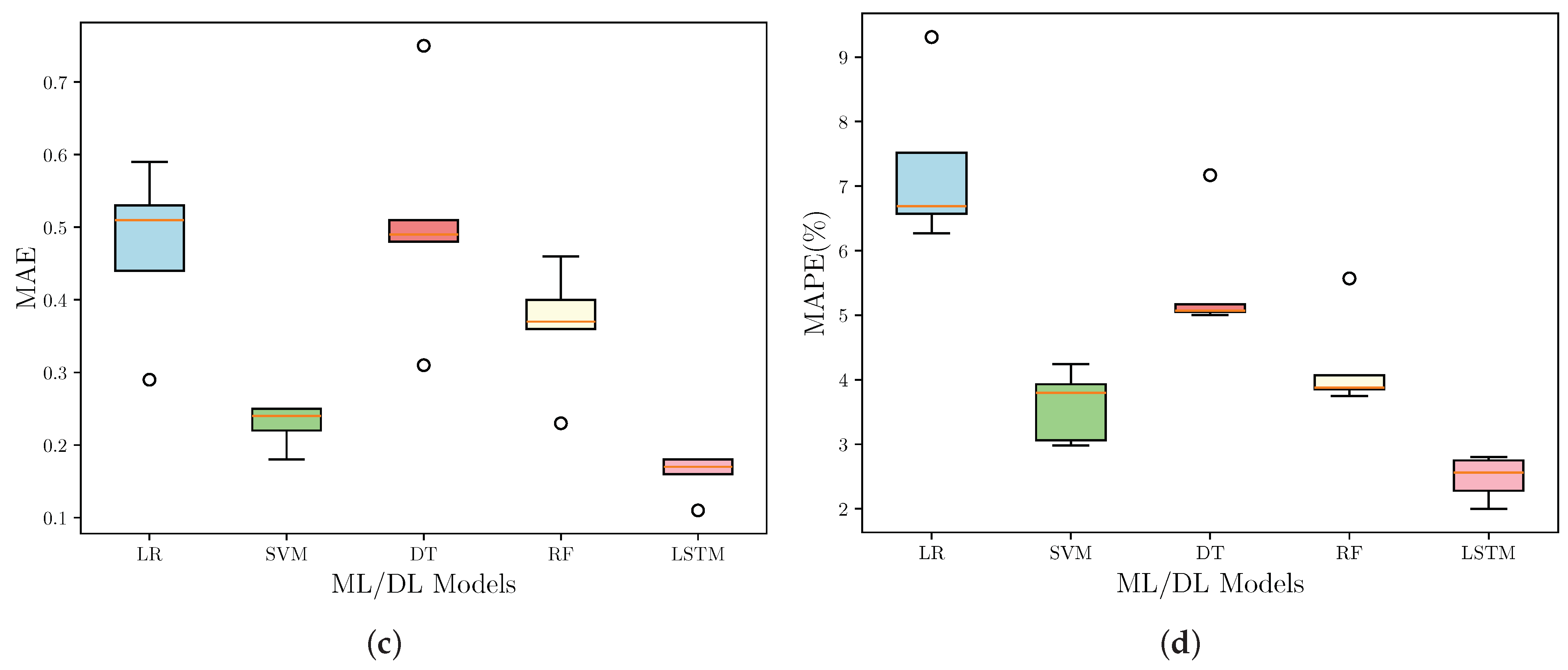
Figure 2 presents a comprehensive comparison of the performance of various ML and DL models, including LR, SVM, DT, RF, and LSTM, using different evaluation metrics for all the regions under consideration. Figure 2a shows the box plot of the MSE values for each model, and we can observe that the LSTM model exhibits the lowest MSE, indicating its superior performance in minimizing the squared differences between predicted and actual values. The DT model, on the other hand, shows the highest MSE, suggesting a poorer fit to the data. The SVM and RF models perform moderately well, with MSE values lower than the DT model but higher than the LSTM model. Figure 2b illustrates the RMSE, which is the square root of the MSE and provides a more interpretable measure of the model’s average prediction error. Consistent with the MSE results, the LSTM model demonstrates the lowest RMSE, followed by the SVM, RF, LR, and DT models, respectively. In Figure 2c, MAE is presented, which measures the average absolute difference between predicted and actual values. The LSTM model again outperforms the other models with the lowest MAE, indicating its ability to minimize the magnitude of prediction errors. The DT model exhibits the highest MAE, while the SVM and RF models perform moderately well. Finally, Figure 2d compares the models based on the MAPE, which expresses the prediction error as a percentage of the actual value. The LSTM model continues to excel, achieving the lowest MAPE, suggesting its superior performance in capturing the relative magnitude of prediction errors. The DT model shows the highest MAPE, indicating a larger relative error compared to the other models.
Based on Figure 2 and Table 2, it is evident that the LSTM model consistently outperformed the other ML and DL models across all evaluation metrics and geographical areas. The LSTM model demonstrated its effectiveness in minimizing prediction errors, achieving higher accuracy, and capturing the long-term dependencies and temporal patterns within the data, which are crucial for accurate forecasting or prediction tasks. Soil moisture data exhibit complex temporal patterns and long-term dependencies, making LSTM’s memory cells crucial for retaining relevant information over multiple time steps. Its sequential data processing capability ensures it captures subtle temporal trends often overlooked by traditional models. Furthermore, LSTMs dynamically adapt to changing patterns, making them robust in capturing non-linear relationships and abrupt changes in soil moisture dynamics. Additionally, they excel at modeling seasonal trends and cyclical patterns inherent in soil moisture data, rendering them superior for accurate time series forecasting of soil moisture estimation. Furthermore, as shown in Table 2, the LSTM model maintained its dominance across various geographic locations, consistently achieving the lowest MSE, RMSE, MAE, and MAPE values in areas such as Cuttack, Kandhamal, Dhenkanal, Talcher, and Angul. This consistency in performance highlights the robustness and adaptability of the LSTM model to different contexts and data patterns.
In contrast, the DT model generally exhibited the poorest performance across both Figure 2 and Table 2. The DT model had the highest MSE, RMSE, MAE, and MAPE values in most cases, potentially due to its tendency to overfit the data or its inability to capture complex patterns effectively. The SVM and RF models performed moderately well, often outperforming the LR model but falling short of the LSTM model’s exceptional performance. This suggests that while SVM and RF models can capture intricate patterns and relationships within the data to some extent, the DL techniques employed by the LSTM model offer a distinct advantage in handling complex, sequential, or time-series data.
Overall, the consistent out-performance of the LSTM model across various evaluation metrics and geographical areas highlights its suitability for accurate forecasting and prediction tasks, particularly in scenarios involving sequential or time-dependent data. Although overfitting can occur if the model memorizes noise in the training data, generalization may be hindered by insufficiently diverse training data. Additionally, meticulous data preprocessing is essential, and training can be computationally demanding. Sensitivity to hyperparameters requires careful tuning, and interpreting model decisions can be challenging due to its black-box nature. Despite these limitations, LSTM models remain powerful tools for capturing temporal dependencies in soil moisture data and making accurate predictions, provided careful attention is given to model development and evaluation.
Additionally, soil moisture estimation models can be compared not only for their predictive accuracy but also for the computing resources they require as shown in Table 3, where n refers to the number of data samples, d refers to the number of input features, T is specific to Random Forests referring to the number of trees, and t represents the number of time steps for LSTM.
Traditional ML algorithms like SVM, Random Forests, Decision Trees, and Linear Regression typically have a time complexity that scales linearly with the number of samples and features, as indicated by the O(nd) time complexity. This suggests that these models can require significant computational resources for feature engineering and training, especially when dealing with large datasets with numerous features. In contrast, the LSTM model has a time complexity of O(tnd), where the additional time step factor t results in higher computational requirements compared to the traditional ML algorithms. This is due to the complex architecture and sequential data processing capabilities of LSTM networks, which demand extensive computational power during the training phase. Despite the higher training time associated with LSTM, its advantages in accuracy and its capacity to capture temporal dependencies in soil moisture data make it a viable option, even if at a greater computational cost. The trade-off between model performance and computational efficiency is an important consideration when selecting the appropriate machine-learning technique for soil moisture estimation tasks.
6. Conclusions and Future Work
In this study, we have explored the utilization of WSNs in conjunction with ML techniques for advancing soil moisture estimation. By leveraging data from WSNs integrated with remote sensing sources such as satellite observations and ground-based sensors, we have demonstrated the effectiveness of ML models in accurately estimating soil moisture content across various geographical regions. Our analysis reveals that models trained on WSN data supplemented with satellite observations exhibit robust performance in estimating soil moisture levels. Specifically, the LSTM model consistently outperforms other ML algorithms across different regions, achieving lower error rates in terms of MSE, RMSE, MAE, and MAPE. The LSTM’s MSE of 0.06 and MAPE of 2.8% indicate a remarkable performance, suggesting that the predicted outcomes closely align with the actual values. The MSE being close to 0 further underscores the accuracy of the predictions, highlighting the model’s ability to minimize the squared differences between predicted and actual values. This underscores the importance of leveraging WSN-driven data to enhance soil moisture estimation accuracy. The findings of our study hold significant implications for agriculture and environmental management. Using the proposed approach, soil moisture can be estimated more accurately. This precision enables optimized irrigation practices, enhancing water use efficiency and crop yields. Moreover, the timely detection of low soil moisture levels facilitates proactive drought mitigation efforts, safeguarding agricultural productivity and rural livelihoods. Additionally, the insights gained support sustainable land management practices, aiding in ecosystem conservation and resilience-building against climate change impacts. It is important to note that our study does not claim to have provided the “best” model for soil moisture estimation [10]. Instead, we aim to offer a comprehensive analysis of the performance of different ML and DL models under similar conditions.
Future research can improve soil moisture estimation models by integrating additional data sources like remote sensing satellites, exploring alternative machine learning algorithms, incorporating climate and environmental factors, and evaluating model uncertainty and robustness. The researchers may focus on the deployment of real-time monitoring systems based on WSNs which can enable continuous monitoring of soil moisture levels, facilitating timely interventions and adaptive management practices. Furthermore, conducting comprehensive validation and calibration studies across diverse environmental conditions and geographical regions will be crucial for ensuring the reliability and applicability of WSN-driven soil moisture estimation models in real-world scenarios.
Author Contributions
T.S.: Writing—original draft preparation, Methodology, data curation. M.K.: Writing—original draft, Conceptualization, Software. T.K.: review and editing, Conceptualization, Supervision. All authors have read and agreed to the published version of the manuscript.
Funding
This research was partly supported by Basic Science Research Program through the National Research Foundation of Korea (NRF) funded by the Ministry of Education (No. NRF-2022R1I1A3072355, 50%) and Innovative Human Resource Development for Local Intellectualization program through the Institute of Information & Communications Technology Planning & Evaluation (IITP) grant funded by the Korea government (MSIT) (IITP-2024-2020-0-01462, 50%).
Data Availability Statement
The datasets generated and/or analyzed during the current study are available from the corresponding author on reasonable request.
Conflicts of Interest
The authors declare that they have no known competing financial interests or personal relationships that could have appeared to influence the work reported in this paper.
References
- Acharya, U.; Daigh, A.L.M.; Oduor, P.G. Machine Learning for Predicting Field Soil Moisture Using Soil, Crop, and Nearby Weather Station Data in the Red River Valley of the North. Soil Syst. 2021, 5, 57. [Google Scholar] [CrossRef]
- Kumar, S.V.; Dirmeyer, P.A.; Peters-Lidard, C.D.; Bindlish, R.; Bolten, J. Information theoretic evaluation of satellite soil moisture retrievals. Remote Sens. Environ. 2018, 204, 392–400. [Google Scholar] [CrossRef] [PubMed]
- Mittelbach, H.; Casini, F.; Lehner, I.; Teuling, A.J.; Seneviratne, S.I. Soil moisture monitoring for climate research: Evaluation of a low-cost sensor in the framework of the Swiss Soil Moisture Experiment (SwissSMEX) campaign. J. Geophys. Res. Atmos. 2011, 116, D05111. [Google Scholar] [CrossRef]
- Mladenova, I.E.; Bolten, J.D.; Crow, W.; Sazib, N.; Reynolds, C. Agricultural drought monitoring via the assimilation of SMAP soil moisture retrievals into a global soil water balance model. Front. Big Data 2020, 3, 10. [Google Scholar] [CrossRef] [PubMed]
- Rajib, M.A.; Merwade, V.; Yu, Z. Multi-objective calibration of a hydrologic model using spatially distributed remotely sensed/in-situ soil moisture. J. Hydrol. 2016, 536, 192–207. [Google Scholar] [CrossRef]
- Saxton, K.E.; Rawls, W.J. Soil water characteristic estimates by texture and organic matter for hydrologic solutions. Soil Sci. Soc. Am. J. 2006, 70, 1569–1578. [Google Scholar] [CrossRef]
- Brady, N.C.; Weil, R.R.; Weil, R.R. The Nature and Properties of Soils; Prentice Hall: Upper Saddle River, NJ, USA, 2008; Volume 13. [Google Scholar]
- Entekhabi, D.; Njoku, E.G.; O’neill, P.E.; Kellogg, K.H.; Crow, W.T.; Edelstein, W.N.; Entin, J.K.; Goodman, S.D.; Jackson, T.J.; Johnson, J.; et al. The soil moisture active passive (SMAP) mission. Proc. IEEE 2010, 98, 704–716. [Google Scholar] [CrossRef]
- Singh, T.; Sharma, N.; Satakshi; Kumar, M. Analysis and forecasting of air quality index based on satellite data. Inhal. Toxicol. 2023, 35, 24–39. [Google Scholar] [CrossRef]
- Singh, A.; Gaurav, K. Deep learning and data fusion to estimate surface soil moisture from multi-sensor satellite images. Sci. Rep. 2023, 13, 2251. [Google Scholar] [CrossRef]
- Orth, R. Global soil moisture data derived through machine learning trained with in-situ measurements. Sci. Data 2021, 8, 1–14. [Google Scholar]
- Romano, E.; Bergonzoli, S.; Bisaglia, C.; Picchio, R.; Scarfone, A. The Correlation between Proximal and Remote Sensing Methods for Monitoring Soil Water Content in Agricultural Applications. Electronics 2023, 12, 127. [Google Scholar] [CrossRef]
- Kumar, M.; Singh, T.; Maurya, M.K.; Shivhare, A.; Raut, A.; Singh, P.K. Quality Assessment and Monitoring of River Water Using IoT Infrastructure. IEEE Internet Things J. 2023, 10, 10280–10290. [Google Scholar] [CrossRef]
- Cai, Y.; Zheng, W.; Zhang, X.; Zhangzhong, L.; Xue, X. Research on soil moisture prediction model based on deep learning. PLoS ONE 2019, 14, e0214508. [Google Scholar] [CrossRef]
- Ge, X.; Wang, J.; Ding, J.; Cao, X.; Zhang, Z.; Liu, J.; Li, X. Combining UAV-based hyperspectral imagery and machine learning algorithms for soil moisture content monitoring. PeerJ 2019, 7, e6926. [Google Scholar] [CrossRef] [PubMed]
- Feng, Y.; Hao, W.; Li, H.; Cui, N.; Gong, D.; Gao, L. Machine learning models to quantify and map daily global solar radiation and photovoltaic power. Renew. Sustain. Energy Rev. 2020, 118, 109393. [Google Scholar] [CrossRef]
- Wu, W.; Zucca, C.; Muhaimeed, A.S.; Al-Shafie, W.M.; Fadhil Al-Quraishi, A.M.; Nangia, V.; Zhu, M.; Liu, G. Soil salinity prediction and mapping by machine learning regression in C entral M esopotamia, I raq. Land Degrad. Dev. 2018, 29, 4005–4014. [Google Scholar] [CrossRef]
- Lu, Z.; Chai, L.; Liu, S.; Cui, H.; Zhang, Y.; Jiang, L.; Jin, R.; Xu, Z. Estimating Time Series Soil Moisture by Applying Recurrent Nonlinear Autoregressive Neural Networks to Passive Microwave Data over the Heihe River Basin, China. Remote Sens. 2017, 9, 574. [Google Scholar] [CrossRef]
- Song, X.; Zhang, G.; Liu, F.; Li, D.; Zhao, Y.; Yang, J. Modeling spatio-temporal distribution of soil moisture by deep learning-based cellular automata model. J. Arid. Land 2016, 8, 734–748. [Google Scholar] [CrossRef]
- Yuan, Q.; Shen, H.; Li, T.; Li, Z.; Li, S.; Jiang, Y.; Xu, H.; Tan, W.; Yang, Q.; Wang, J.; et al. Deep learning in environmental remote sensing: Achievements and challenges. Remote Sens. Environ. 2020, 241, 111716. [Google Scholar] [CrossRef]
- Adab, H.; Morbidelli, R.; Saltalippi, C.; Moradian, M.; Ghalhari, G.A.F. Machine learning to estimate surface soil moisture from remote sensing data. Water 2020, 12, 3223. [Google Scholar] [CrossRef]
- Leng, P.; Yang, Z.; Yan, Q.Y.; Shang, G.F.; Zhang, X.; Han, X.J.; Li, Z.L. A framework for estimating all-weather fine resolution soil moisture from the integration of physics-based and machine learning-based algorithms. Comput. Electron. Agric. 2023, 206, 107673. [Google Scholar] [CrossRef]
- Villegas-Ch, W.; García-Ortiz, J. A Long Short-Term Memory-Based Prototype Model for Drought Prediction. Electronics 2023, 12, 3956. [Google Scholar] [CrossRef]
- Sazib, N.; Bolten, J.D.; Mladenova, I.E. Leveraging NASA Soil Moisture Active Passive for Assessing Fire Susceptibility and Potential Impacts Over Australia and California. IEEE J. Sel. Top. Appl. Earth Obs. Remote Sens. 2022, 15, 779–787. [Google Scholar] [CrossRef]
- Mladenova, I.E.; Bolten, J.D.; Crow, W.T.; Sazib, N.; Cosh, M.H.; Tucker, C.J.; Reynolds, C. Evaluating the Operational Application of SMAP for Global Agricultural Drought Monitoring. IEEE J. Sel. Top. Appl. Earth Obs. Remote Sens. 2019, 12, 3387–3397. [Google Scholar] [CrossRef]
- Sazib, N.; Mladenova, l.E.; Bolten, J.D. Assessing the Impact of ENSO on Agriculture Over Africa Using Earth Observation Data. Front. Sustain. Food Syst. 2020, 4, 509914. [Google Scholar] [CrossRef]
- NASA Power Data Access Viewer. Available online: https://power.larc.nasa.gov/data-access-viewer/ (accessed on 18 February 2024).
- IMD Pune. Available online: https://dsp.imdpune.gov.in/ (accessed on 18 February 2024).
- NASA. SMAP: Soil Moisture Active Passive Mission; National Aeronautics and Space Administration. Available online: https://smap.jpl.nasa.gov/ (accessed on 18 February 2024).
- Zhang, Z. Multiple imputation with multivariate imputation by chained equation (MICE) package. Ann. Transl. Med. 2016, 4, 1–5. [Google Scholar]
- LaValle, S.M.; Branicky, M.S.; Lindemann, S.R. On the relationship between classical grid search and probabilistic roadmaps. Int. J. Robot. Res. 2004, 23, 673–692. [Google Scholar] [CrossRef]
Figure 1.
Methodology overview for soil moisture estimation via WSN-driven ML approaches.

Figure 2.
Comparison of model performance using (a) MSE, (b) RMSE, (c) MAE, and (d) MAPE for LR, SVM, DT, RF, and LSTM models.
Figure 2.
Comparison of model performance using (a) MSE, (b) RMSE, (c) MAE, and (d) MAPE for LR, SVM, DT, RF, and LSTM models.


Table 1.
Optimal hyper-parameters for models identified through grid search.
| Model | Hyper-Parameter | Search Space | Optimal Value |
|---|---|---|---|
| LR | None | None | None |
| SVM | C | {0.1, 1, 10, 100, 1000} | 10 |
| Gamma | {0.0001, 0.001, 0.01, 0.1, 1} | 0.001 | |
| DT | Max depth | {2, 3, 5, 10, 20} | 3 |
| Min samples leaf | {5, 10, 20, 50, 100} | 50 | |
| RF | B | {25, 50, 100, 150} | 25 |
| LSTM | Learning rate | {0.001, 0.01, 0.1, 0.2} | 0.001 |
| Batch Size | {8, 16, 32, 64} | 32 | |
| Dropout | {0.2, 0.3, 0.4} | 0.3 | |
| Optimizer | {SGD, RMSprop, Adam} | Adam |
Table 2.
Location-wise performance of different models using varied matrices.
| Location: | Cuttack | |||
|---|---|---|---|---|
| Model | MSE | RMSE | MAE | MAPE |
| LR | 0.59 | 0.77 | 0.51 | 7.52% |
| SVM | 0.26 | 0.51 | 0.25 | 4.24% |
| DT | 1.02 | 1.01 | 0.75 | 7.17% |
| RF | 0.69 | 0.83 | 0.46 | 5.57% |
| LSTM | 0.06 | 0.24 | 0.16 | 2.80% |
| Location: | Kandhamal | |||
| LR | 0.53 | 0.73 | 0.53 | 6.69% |
| SVM | 0.27 | 0.52 | 0.25 | 2.98% |
| DT | 0.94 | 0.97 | 0.48 | 5.05% |
| RF | 0.47 | 0.68 | 0.36 | 3.75% |
| LSTM | 0.08 | 0.28 | 0.18 | 2.00% |
| Location: | Dhenkanal | |||
| LR | 0.2 | 0.45 | 0.29 | 6.57% |
| SVM | 0.2 | 0.44 | 0.18 | 3.93% |
| DT | 0.56 | 0.75 | 0.31 | 5.00% |
| RF | 0.26 | 0.51 | 0.23 | 3.88% |
| LSTM | 0.03 | 0.17 | 0.11 | 2.56% |
| Location: | Talcher | |||
| LR | 0.37 | 0.61 | 0.44 | 6.27% |
| SVM | 0.18 | 0.42 | 0.22 | 3.06% |
| DT | 0.78 | 0.89 | 0.49 | 5.17% |
| RF | 0.46 | 0.68 | 0.37 | 3.85% |
| LSTM | 0.06 | 0.24 | 0.17 | 2.28% |
| Location: | Angul | |||
| LR | 0.76 | 0.87 | 0.59 | 9.31% |
| SVM | 0.26 | 0.51 | 0.24 | 3.80% |
| DT | 0.96 | 0.99 | 0.51 | 5.07% |
| RF | 0.49 | 0.72 | 0.40 | 4.07% |
| LSTM | 0.05 | 0.21 | 0.18 | 2.75% |
Table 3.
Computational cost of different models used in this study.
| Model | Time Complexity |
|---|---|
| Linear Regression | O(nd) |
| Support Vector Machine | O(nd) |
| Decision Tree | O(ndlog(n)) |
| Random Forest | O(Tndlog(n)) |
| LSTM | O(tnd) |
Disclaimer/Publisher’s Note: The statements, opinions and data contained in all publications are solely those of the individual author(s) and contributor(s) and not of MDPI and/or the editor(s). MDPI and/or the editor(s) disclaim responsibility for any injury to people or property resulting from any ideas, methods, instructions or products referred to in the content. |
© 2024 by the authors. Licensee MDPI, Basel, Switzerland. This article is an open access article distributed under the terms and conditions of the Creative Commons Attribution (CC BY) license (https://creativecommons.org/licenses/by/4.0/).
Share and Cite
MDPI and ACS Style
Singh, T.; Kundroo, M.; Kim, T. WSN-Driven Advances in Soil Moisture Estimation: A Machine Learning Approach. Electronics 2024, 13, 1590. https://0-doi-org.brum.beds.ac.uk/10.3390/electronics13081590
AMA Style
Singh T, Kundroo M, Kim T. WSN-Driven Advances in Soil Moisture Estimation: A Machine Learning Approach. Electronics. 2024; 13(8):1590. https://0-doi-org.brum.beds.ac.uk/10.3390/electronics13081590
Chicago/Turabian StyleSingh, Tinku, Majid Kundroo, and Taehong Kim. 2024. "WSN-Driven Advances in Soil Moisture Estimation: A Machine Learning Approach" Electronics 13, no. 8: 1590. https://0-doi-org.brum.beds.ac.uk/10.3390/electronics13081590
Note that from the first issue of 2016, this journal uses article numbers instead of page numbers. See further details here.