Article

Software-Defined Networking-Enabled Efficient Default Route Configuration in IEEE 802.15.4 Protocol: A Smart Algorithmic Approach

by
Carlos Egas Acosta
,
Luis Criollo
,
Christian Tipantuña
* and
Jorge Carvajal-Rodriguez
Department of Electronics, Telecommunications, and Computer Networks, Escuela Politécnica Nacional, Quito 170525, Ecuador
*
Author to whom correspondence should be addressed.
Submission received: 15 December 2023 / Revised: 20 January 2024 / Accepted: 22 January 2024 / Published: 18 April 2024

Abstract

:
Today’s software-defined networking (SDN) applications have many challenges. Its main applications are focused on networks with nodes with high processing capacity. Applying SDN technology in nodes operating on batteries with limited computing capabilities is challenging. In this context, this paper proposes SDN-enabled algorithms for the remote configuration of the default route to be applied in multi-hop wireless sensor networks (WSNs) with tree-type topology using the IEEE 802.15.4 protocol. The routing algorithm to define the default route of each node is executed in an SDN-enabled WSN controller (SDWSN). The SDWSN controller receives information on the state of the network, executes the Djikstra or Kruskal algorithms, and configures the default route of the nodes remotely. The best route selection is based on the battery level of the nodes and the distance between them. The results show that using network protocols to configure the nodes remotely is unnecessary.

1. Introduction

Wireless sensor networks (WSNs) are a fundamental factor in the growth and development of new applications for IoT networks [1]. WSNs allow for the development of monitoring applications associated with smart cities, factories, and surveillance systems [2,3]. Implementing multi-hop wireless sensor networks presents a significant challenge due to the energy consumption of the relay nodes and the end-to-end delay [4].
Software-defined networking (SDN) is an architecture proposed for networks in which the processes carried out in the network are grouped into two planes: (i) the control plane that determines the traffic routes and (ii) the data plane that forwards the traffic packets [5]. WSNs are different from the conventional networks that SDN was initially designed for. The use of SDN in WSNs is known as software-defined wireless sensor networking (SDWSN), where all the processes a node performs are executed centrally in the controller [6]. WSNs have limited resources, so developing SDWSNs becomes a challenge due to inherent restrictions in the WSN architecture.
Integrating WSN and SDN lies in pursuing enhanced network efficiency, reducing processing delays, and following our previous works [7,8] in which the network layer performance uses solely link layer information. The SDN paradigm facilitates implementation in WSN due to the low computing capacity of the nodes.
The calculation limitations of the nodes of a WSN generate delay times for processing when routing algorithms are executed [9] to find the default route of the nodes. This constraint hinders the application of internet network architecture to WSNs, primarily due to elevated processing delays. Various network architectures are presently employed in developing WSN applications [10], with ongoing adaptation and development of protocols for this network type. Consequently, addressing the challenge of minimizing processing delays at WSN nodes remains a significant concern. In addition, the energy consumption for processing affects the lifetime of the nodes because they run on batteries [11]. The 6LowPAN protocol allows information from the nodes to reach the controller and the controller to configure the nodes remotely [12]. This protocol, derived from IPv6 for WSN, faces extended convergence times in multi-hop scenarios. Employing SDN technology in an SDWSN network facilitates the utilization of a controller for configuring the network, ensuring swift convergence times for the default route of the nodes. The execution of the routing algorithm is not a problem due to the processing capabilities of the controller; however, minimizing the transmission delays to and from the controller with the nodes is a challenge due to the network protocols used in WSN.
Routing control between the sensor node and the gateway in a multi-hop topology using SDWSN controllers is critical because it must be adequate, adaptable, and reliable. Several architectures are currently operating for WSNs [10]. SDN allows us to have a unique architecture, resolve processing delays, minimize node energy consumption, and facilitate new application creation. In an SDN, routing management performed by the controller allows for higher QoS and longer network life. Failures in WSNs frequently occur due to connectivity disruptions, power shortages, changes in environmental conditions, and other disruptive events. Therefore, the network must be configured, managed, and maintained for self-healing and fault tolerance. Using a controller results in a robust feature that allows the WSN to provide useful information even when some failed nodes and links modify the network topology.
Routing management in the WSN must support node mobility, resulting in topology changes, including handling unreliable wireless links. Considering the need to develop technology in the area of SDWSNs, which optimizes the delays between the controller and the nodes due to the processing delay in the node, the use of the IEEE 802.15.4 protocol is proposed, without the use of network and transport to transport information that allows the controller to calculate the default route of each node and configure this parameter for the nodes remotely. Dijkstra [13] and Kruskal [14] algorithms define the route between the sensor node and the gateway and, therefore, the default node to which the sensor node should transmit data. In this context, an algorithmic solution is proposed that allows the transmission of information between the controller and the sensor nodes using the 802.15.4 protocol as a data transport protocol so that the controller finds the optimal tree-type topology and defines the best route between the sensor node and the gateway. In summary, this work has the following features:
  • Use of an SDN-enabled controller that reduces the processing delay in the node.
  • The best route selection is based on node battery level and distance between nodes.
  • Use of IEEE 802.15.4 protocol for data transport between the sensor node and the controller.
  • Proposal of an SDWSN architecture without network-level protocols.

2. Related Work

The importance of routing in WSNs and its impact on the implementations is discussed in several works in the literature [15], even considering energy concerns [16]. Likewise, the use of SDN in WSN is explored in some contributions, for instance, in [17]. Several researchers discuss routing control for SDWSN using computational methods. In [18], the authors analyze the advantages of using a centralized SDN control to plan network routes in which the OpenFlow protocol is used to monitor the routing status and link the routing information of network load in real-time. The routes are obtained using the Elman neural network. In [19], SDN-WISE improves routing processes in WSN operating with TSCH. Instead, reinforcement learning techniques to select the best path in an SDWSN are used in [20], considering all the necessary metrics to have energy efficiency and the QoS of the WSN.
In [21], the Kruskal and clustering algorithms select each group’s nodes to increase the network’s lifetime. Similarly, in [22], the algorithm of Kruskal is used to determine the route within a group of nodes and thus optimize energy consumption. The Dijkstra algorithm is used in SDN in [23,24] for routing control and uses complex metrics to select the best route, including hop count and energy efficiency. In [25], the algorithm for reliable networks is applied by selecting nodes with the lowest transmission power to route data between networks and comparing it with the LEACH algorithm.
Table 1 shows related work focused on the routing problem in SDWSN by implementation or through simulation. A notable observation is that most of the proposals use simulation tools, but in contrast to the works implemented, nodes use high processing capacity due to the complexity of the algorithms.

3. Proposed Algorithmic Approach

This section describes the algorithm implemented in the sensor nodes for information transfer between the controller and the nodes using the protocol IEEE 802.15.4. The nodes send the information to the controller, and the controller calculates the optimal topology of the best route for each node and sends the default route or default node to each sensor node. The relay nodes with the most energy in the batteries and the shortest distance between relay nodes are considered to select the best route. Nodes store their battery level, along with the identifiers of neighboring nodes and the corresponding received signal levels. This information is transmitted to the controller for algorithm execution.
The network diagram used to perform performance tests of the algorithms is shown in Figure 1. The prototype is minimally feasible regarding the number of nodes, but it facilitates algorithm testing, assuming that node identifiers are pre-assigned and tested in controlled scenarios. The network consists of eight ATZB256RFR2 wireless nodes, separated from each other by a distance of 15 cm. These nodes will be assigned the default route generated in the application. The absence of implemented link layer neighbor discovery protocols and network layer routing protocols in the nodes prevents them from determining nodes within their coverage area and identifying the controlling node for direct transmission. Consequently, test scenarios can be created where intermediate nodes relay data, forming a multi-hop network. The communication between nodes is defined by software, enabling emulation of scenarios without communication due to being out of coverage zones. This setup facilitates nodes within the sniffer’s coverage area to capture frames from all nodes, assessing the algorithm’s performance. The nodes are exclusively programmed for operation with the 802.15.4 protocol, with libraries enabling direct frame manipulation. Before algorithm testing, nodes are set up in a predetermined multi-hop topology, programmed to communicate with predefined nodes exclusively. The default route is established, ensuring nodes know the designated relay node for initial data transmission to the controller node. Subsequently, the controller dispatches frames to nodes, enabling each to store reception intensity levels from previously designated neighboring nodes. With these preparations completed, the prototype is poised for validating the proposed algorithm’s functionality.
The nodes maintain operational status with average voltage values ranging from a maximum of 2.8 V to a minimum of 1.8 V, supplied by two AAA batteries. In the conducted tests, it is assumed that the transmit power levels of the nodes remain constant irrespective of the battery level. Consequently, we can infer that a lower reception signal level under a consistent transmit power indicates a greater distance from the node.
In Figure 1, node 8, with address 0x0008, acts as a controller node and is responsible for transporting the generated frames to the computer so that the latter can execute the corresponding algorithms. This node is also responsible for sending the new default route from the application once the user decides. This information must be sent along with the node’s source address within the payload of an IEEE 802.15.4 frame. The information must reach the controller node through a default route and subsequently to the application. The computer is also connected to the sniffer, which allows viewing the frames sent between the nodes and measuring the transmission time of the frames between them.

3.1. Route Generator Application

Figure 2 shows the application in charge of generating new routes by default; it has been developed in the PyCharm integrated development environment using the Python 3.9.0 programming language and the QT Designer tool.
The application was designed to obtain and send data from a controller node using a serial communication interface (USB to UART CP210x). The application integrates the codes corresponding to the Kruskal and Dijkstra algorithms. Based on graph theory, these algorithms have been adapted to receive information from the wireless network. They require vertices, edges, and weights. Therefore, an adaptation is carried out where the nodes represent the vertices, the wireless connections between nodes represent the edges, and the combination of the battery level with the received signal level represents the weights. The information the application receives is displayed on the screen and processed to execute the Kruskal or Dijkstra algorithm. The number of vertices and edges processed will be displayed. Once the algorithms have been implemented, the new default route will be presented in a new window, which can be sent to the wireless network through the communication interface and the controller node.
For the development of the application, the flow diagram represented in Figure 3 is used. In this diagram, the interaction between the route-generating application and the ATZB-256RFR2 nodes is observed, especially with the node that functions as a controller. The application listens to the COM communication port to receive data from some node (neighbors_Table). This completes the application’s neighborsTableList. Once the list above contains sufficient data, the application processes it to verify the information necessary to apply an algorithm. Subsequently, it converts this data into numerical values that can be used to execute the algorithms. The results are stored in the nodesAndWeightsList. If there is no necessary data, the application restarts the lists. When the required data is available, the execution of the Kruskal or Dijkstra algorithm should be selected. By choosing any of the algorithms, the application executes them and generates a new route, which is stored in its respective list (defaultRouteKruskal or defaultRouteDijkstra). With the generated route, the application sends this information to the controller node, which is responsible for transmitting it to the corresponding nodes. Once the new route has been sent, the application empties the data from all the lists, thus avoiding conflicts when executing the algorithms again. For a detailed view of the application and node configuration, readers can access the respective repositories [30,31].

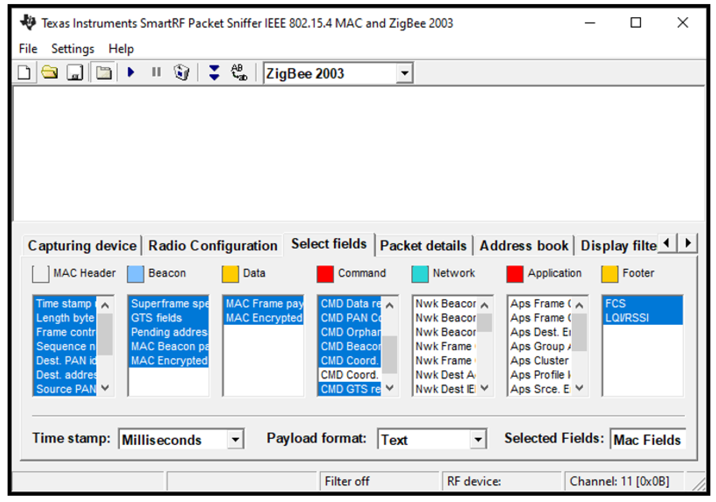
3.2. SmartRF Packett Sniffer

SmartRF Packet Sniffer is a software application developed by Texas Instruments (Dallas, TX, USA) to view IEEE 802.15.4 frames captured through a radio frequency receiver, as shown in Figure 4. This tool provides functionality to filter, decode, and present data and options to filter and store information in binary format. The packet sniffer works with the CC2531 radio frequency receiver for its correct operation, which must be connected to the computer through a USB connection. In addition, it is important to mention that the application is compatible with Windows 7 and Windows 10 operating systems.

3.3. CC2531 USB Hardware

Texas Instruments offers the CC2531 USB dongle (see Figure 1) and corresponding documentation to support a PC interface in IEEE 802.15.4/ZigBee applications. The dongle can be connected directly to your PC and used as an IEEE 802.15.4 packet sniffer, among other purposes. With the CC2531 USB firmware library available online, developing your software to operate this device is possible. An external programmer is required to program the debugger. Both the software and the hardware allow for the verification of the information sent from the nodes to the route-generating application and vice versa. In addition, verifying the new routes that algorithms generate through the Packet Sniffer application is possible. This is achieved by observing the similarity between the source and destination addresses of the 802.15.4 frames presented in both applications.

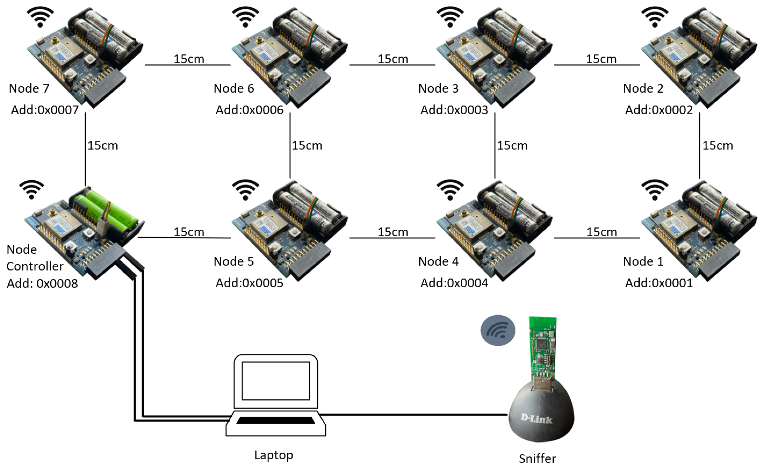
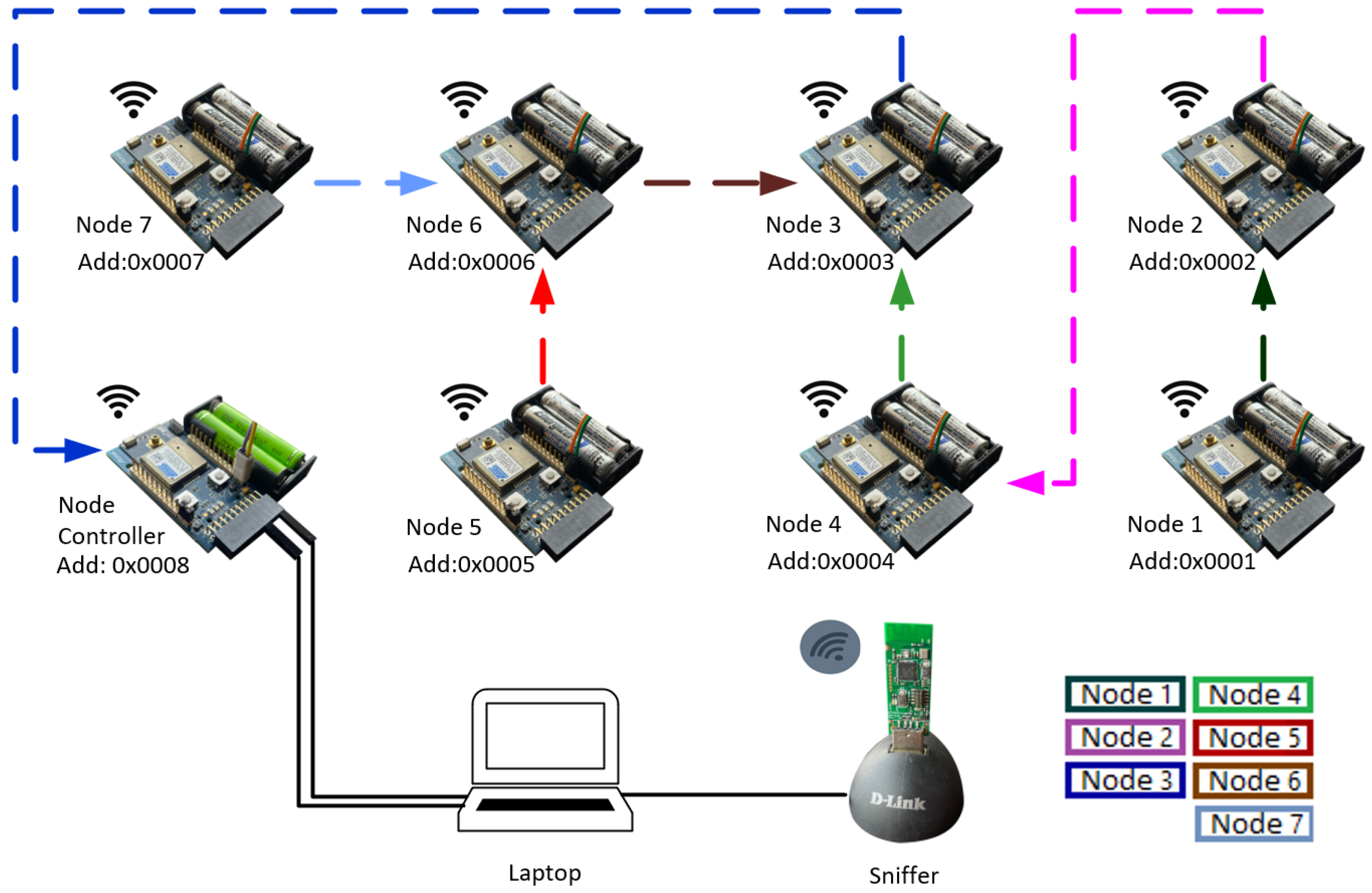
3.4. Operation of the Route Generator Application within the Network Prototype

When the application runs on the computer and the controller node is connected via the USB serial interface, sending a test frame using the “Send” button is possible. This frame will be visible from the sniffer application. After sending the frame, a list will be displayed, allowing the application to view the data received through the controller, as shown in Figure 5. If the above steps have been completed, it can be assumed that the controller is connected correctly. If the controller is connected correctly and can receive information from other nodes, it is already possible to send information from any node via its send button. Through the application’s reception controls, select the device from which you want to receive data, which in this case is a node. The application will wait until it receives the frame with the requested information. The information sent can be verified through the sniffer. After transmitting the initial frame, the nodes retransmit it throughout the network and store the information about the energy and signal levels in memory.
The stored information must be sent to the application through the push button of each node once a Dijkstra or Kruskal algorithm needs to be executed. The information received (neighbor table) is displayed in the application, where the address of the node containing the information (ID_S), the battery level (NB), and the signal quality (NS) of the nodes within range, together with their respective address (ID_S_NS), can be observed. Once the application has received all the information sent by the nodes and the controller, processing needs to be performed using the “Process” button to evaluate if the stored information is adequate to run the algorithms. All the above is shown in Figure 6a.
Once the processing is complete, the application will generate the edges using the directions and weights derived from the battery level and signal quality information. The total number of nodes and edges generated during processing will be displayed in the application. In addition, selecting the algorithm to be executed will be allowed. After selecting the desired algorithm, new routes will be generated and displayed on an additional screen, as shown in Figure 6b. It will be possible to send these new routes to each node through a broadcast transmission from this window. Through the application and the controller, frames containing an End Destination Identifier (ID_DF), a Default Identifier (ID_DEFAULT), and a Frame Identifier (ID_FRAME) will be sent.
The nodes will verify the Final Destination Identifier and modify the node’s destination address to the Default Identifier if it matches the node’s source address. Otherwise, they will retransmit the information if they have not previously stored the identifier of the received frame.
The decision of knowing how far or close the node is at present is based on the reception power of the frame that arrives at the node. The controller, with the information about the neighbors of each node, executes the routing algorithms to define the network’s topology, determine the best route, and define the default node for each sensor node. From the best routes found, each node is sent the identifier of the destination node to which it must send the frames so that they reach the gateway and, thus, the controller. The proposed algorithm to operate in multihop networks that use the IEEE 802.15.4 protocol considers the following scenario:
  • Sensor nodes are fixed.
  • There are several nodes within the coverage area of each node.
  • Topology changes occur by adding or removing a node in the network.
  • The nodes are configured to operate in non-slotted mode with the IEEE 802.15.4 standard (FFD) and do not utilize network-layer protocols or operating systems.
  • The controller updates the route periodically at times defined at the beginning.
Obtaining the default route node default includes three stages: (i) the data collection stage of each node’s battery and received signal strength levels; (ii) the execution stage of the Kruskal or Dijkstra algorithm in the controller; and (iii) the stage where the controller sends the default route to each node. Algorithm 1 defines the following variables and is executed in sensor nodes:
  • ID_S: Identifier of the node that sends the neighbor table to the controller. This identifier is also stored within IEEE802.15.4 frames.
  • NB: Node battery level.
  • NS: Frame receive power level.
  • ID_D: Identifier of the predefined route, located in each node. This identifier is also stored within IEEE802.15.4 frames.
  • ID_DF: Node identifier of the node to which the predefined route will be modified. This identifier is also stored within IEEE802.15.4 frames.
  • SRC_ADDR: Source node address.
  • DST_ADDR: Destination node address.
  • Neighbor_table: Stores NB, NS, and ID_S. This table is also stored within IEEE802.15.4 frames.
  • Uplink_frame: Indicates whether a frame travels on an uplink or downlink.
Algorithm 1: Sensor node pseudocode.
Electronics 13 01537 i001
Algorithm 2 is instead implemented in the controller and calculates the default routes for each node within the network.
Algorithm 2: Controller node pseudocode.
Electronics 13 01537 i002

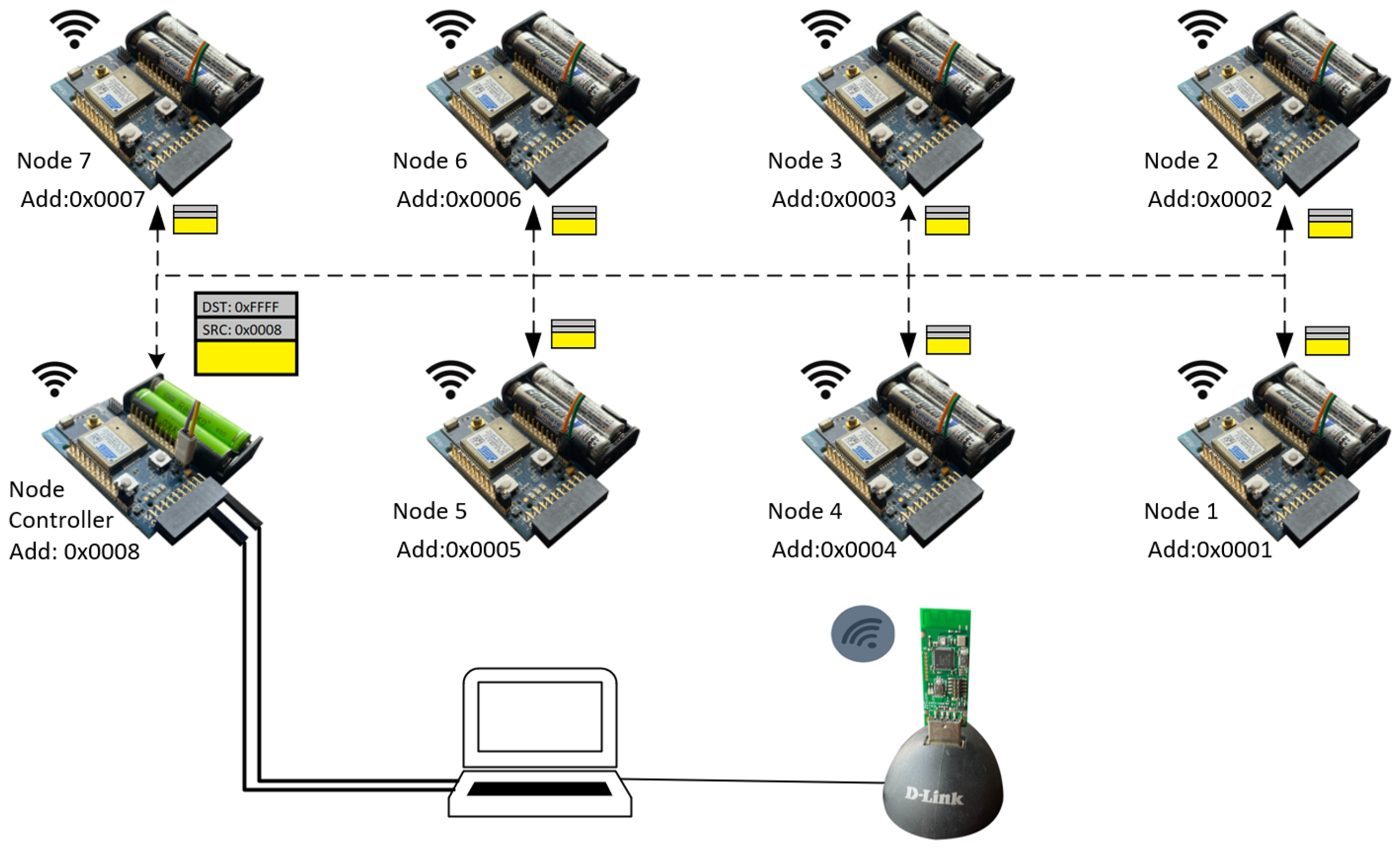
3.5. Uplink and Downlink

For algorithm execution, a wireless network is configured with nodes capable of receiving and transmitting frames from nearby nodes, emulating a multi-hop tree topology. This involves defining uplinks and downlinks: the uplink facilitates the flow of frames from nodes to the controller node, while the downlink enables frames from the controller node to reach each networked node. Initially, the downlink allows for the neighbor tables of each node to be populated. After executing the algorithms, this link will allow you to reconfigure a new default route. The uplink makes it possible to send the neighbor tables, with the information necessary for executing the Kruskal and Dijkstra algorithms, to the controller node and then to the route-generating application. Subsequently, it allows for verifying the operation of the algorithms. This link depends on the default route configured on the nodes.

3.6. Default Route

The default route refers to the path that the data generated by the nodes will follow once the application performs the routing process, which is to say, the selection of the best path as shown in the example in Figure 7. The default route depends on the source and destination address of each node. Therefore, it is important to note that the source address cannot be modified, while the destination address can vary depending on the default route. The application assigns the destination address of each node based on the execution of each algorithm. Depending on the algorithm, this default route can be adjusted according to each node’s battery level and received signal quality.

3.7. Initial Default Route

Because there is not enough information available to execute any algorithm, it is necessary to configure an initial default route that connects all the nodes in a linear manner, which causes a separation of 15 cm between them. Once each node has the necessary information for the controller to run the algorithm, a push button is used to transmit each node’s neighbor tables. When activated, it generates a frame that jumps from node to node until it reaches the controller, as shown in Figure 8.
The transmission times between nodes when communicating through the initial default route were measured to compare algorithms and determine the most efficient. Considering the separation distance and the initial configuration of the default route, the nodes communicate linearly, with a separation distance of 15 cm between them. Measurements of the initial default route reveal that a frame originating from the node furthest from the controller (node 1) takes 42 milliseconds, considering 6 relay nodes in which the source node is included and a delay time in each node of 6 msec, to reach the controller node. Each node’s average retransmission time, totaling six milliseconds, encompasses propagation time, frame transmission time (TF), frame processing ( T F P ) time, backoff time ( T B O ), time to switch from receiver to transmitter ( T T A ), and the duration required to detect a busy channel ( T C A ), as depicted in Figure 9. Notably, propagation time is significantly shorter compared to the other time components, and the average values obtained account for various backoff times in scenarios where two nodes seek access to the channel.
The time recorded by the sniffer denotes the moment when the frame arrives and is stored for processing, excluding the duration from when the frame departs the source node and the propagation time. It is important to note that the subsequent measurements at the next node encompass these times, including the frame’s departure from the source node and the propagation time. This consistency is maintained across all retransmissions due to the test scenario.
The measurement of the transmission time of a frame traveling through the initial default path is considered a reference to compare the performance of the nodes with and without the application of the algorithm.

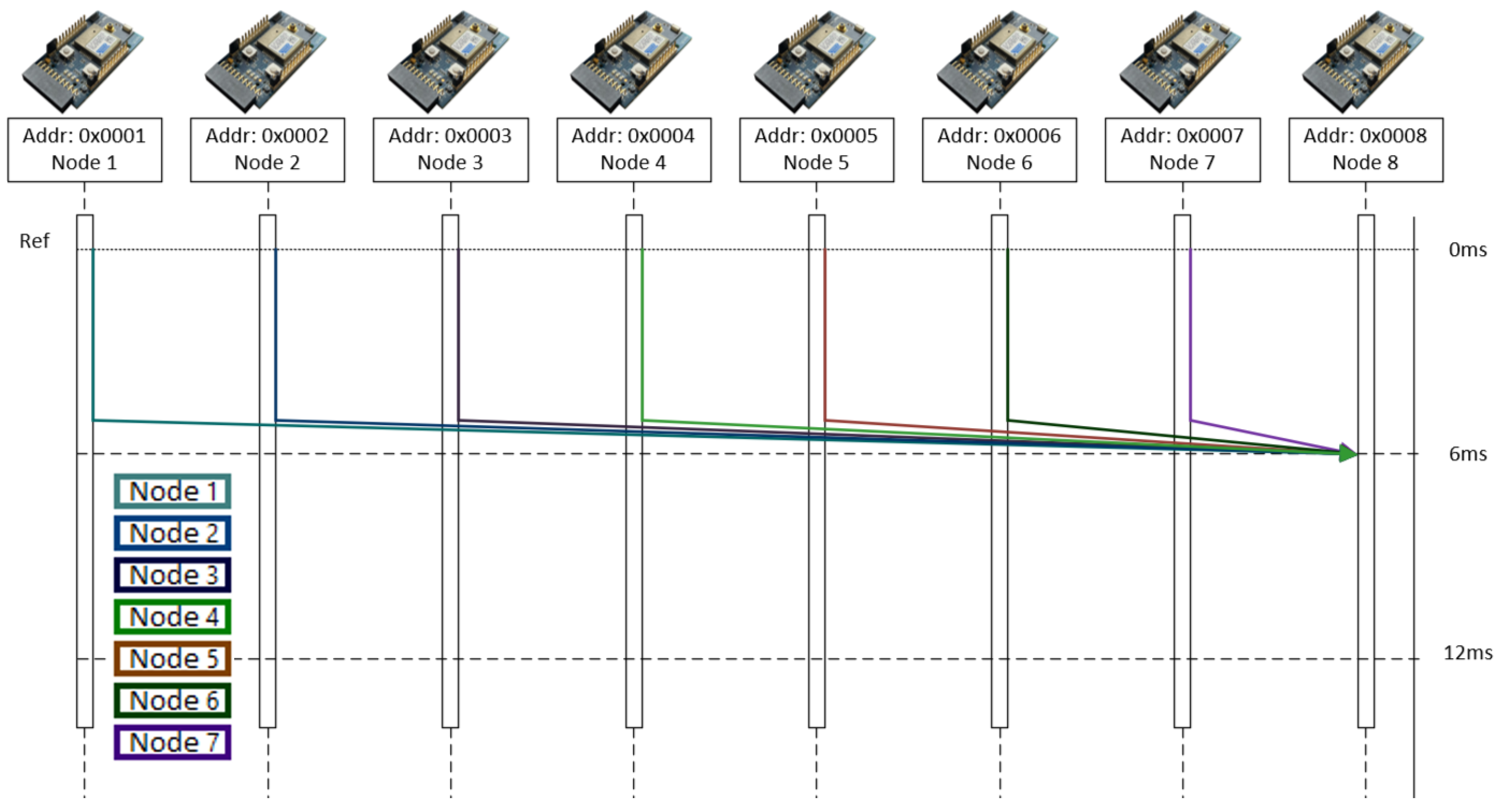
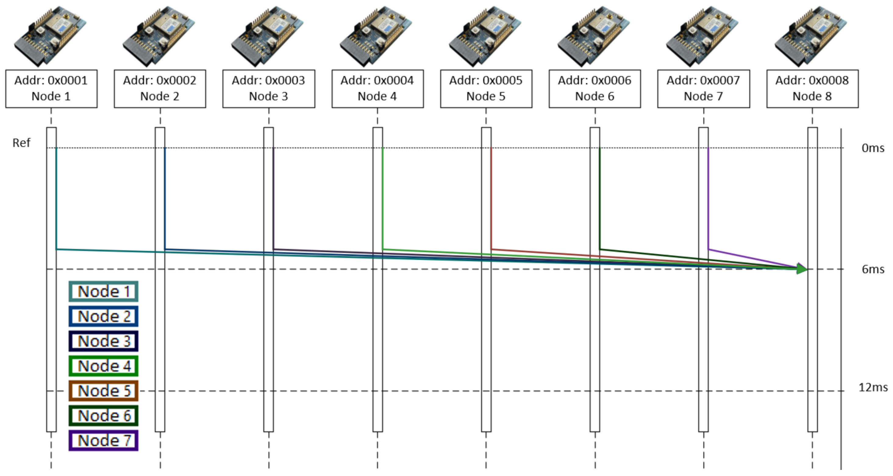
3.8. Exchange of Initial Information

Because the algorithms depend on nodes (vertices), edges (connections between nodes), and weights (battery level and received signal quality), information is required to be sent from the controller to all nodes using a broadcast frame (0xFFFF) and a downlink. The broadcast frame is transmitted and propagates throughout the network through this link and an application, as shown in Figure 10. The receiving nodes store this frame and retransmit it to their nearby nodes, which allows for its propagation in the network, as shown in Figure 11. In this way, all nodes that receive a frame with destination address 0xFFFF must retransmit the information until it reaches all nodes in the network. This broadcast frame allows each node to identify the nodes within its coverage range. Once the retransmission is complete, each node will have information about the battery level and signal quality of all the nodes it can reach.
Figure 12 shows several captured frames sent from the network’s nodes to the controller node. These frames contain information on the node’s battery and energy levels in their payload (neighbors table). For example, in the payload of the first frame, the first two bytes indicate the node’s address that sends the neighbor table (00 07—0x0007). The next four bytes represent the battery level (33 2E 31 35—3.15v). Subsequent bytes represent the energy levels of frames previously received by the node and the node’s source address that generated them. Thus, the seventh to the tenth byte indicates the reception of a frame with an energy level of 00 30, which was transmitted by node 0x0008 (00 08).

4. Results

This section presents the outcomes of implementing the SDN-enabled algorithms for remote default route configuration in IEEE 802.15.4-based multi-hop wireless sensor networks. The experiments aimed to showcase the effectiveness of the proposed algorithm.

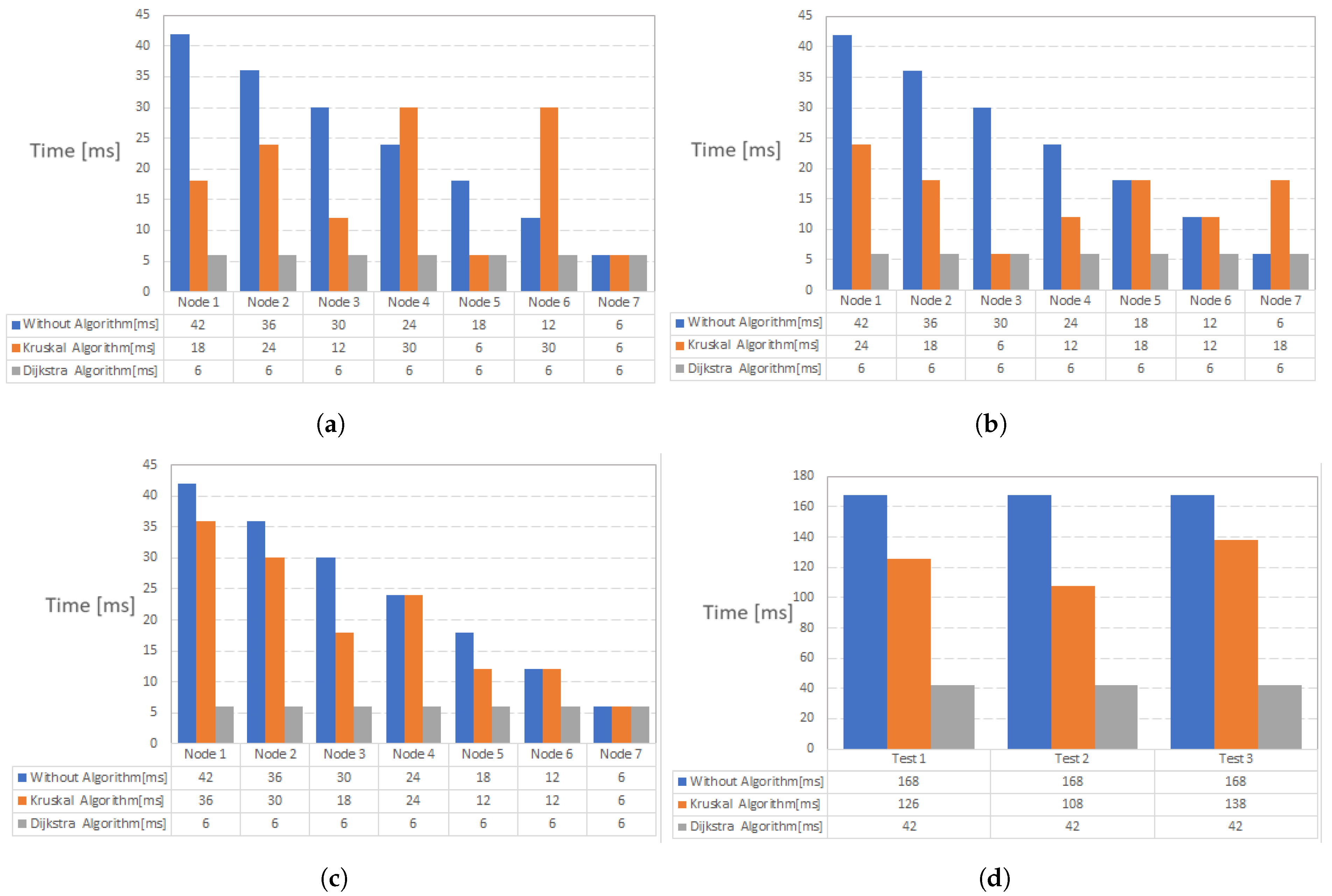
4.1. Results with Kruskal’s Algorithm

Figure 13a shows the values obtained by the controller when executing the Kruskal algorithm. In this case, it can be seen that the controller must send the information of its default route to each node. For instance, node 0x0004 has its default route equal to 0x002. The controller sends broadcast frames to each node; the value of the default route I D D and the value of the node to which the I D S information is directed is in the payload. Figure 13b shows the broadcast frames with the values obtained with the Kruskal algorithm sent to each node.
It is also important to note that the nodes’ batteries present similar voltage values (around 2.55 V) in this test, resulting in similar signal levels (between 0x002D and 0x003B). Using Kruskal’s algorithm, the test generates a route that connects all the wireless network nodes. As a result, the controller will receive frames that follow the new default route. The latter can be verified in Figure 14. Additionally, you can observe a change in the initial default route to a completely different one. This new default route connects all nodes. The nodes closest to the controller relay information from the more distant nodes. The reconfiguration of each node’s source and destination addresses is identical to what is shown in the application (see Figure 13a).

4.2. Results with Dijistra’s Algorithm

Figure 15a shows the values obtained by the controller when executing the Dijkstra algorithm. Figure 15b shows the broadcast frame that the controller sends to each node with the values obtained from the default route with the Dijkstra algorithm. The frames sent to four nodes are presented in the same way the payload contains the data of the node identifier and the default route.
For this test, similar voltage values (approximately 2.55 V) and signal levels between 0x002D to 0x003B obtained for executing the Kruskal algorithm are used. The test is conducted by requesting the application to generate a new default route using Dijkstra’s algorithm. This algorithm creates a default route where the priority is to connect each node to the controller node. In this test, as seen in Figure 16, the information generated by each node does not go through intermediate nodes to reach the controller. Because this algorithm prioritizes the direct connection of the nodes to the controller, a path similar to a star topology is generated.

4.3. Results Using a Pair of Nodes with Voltage Values Higher than the Others

This subsection presents results where the battery voltage values of the nodes are considered.

4.3.1. Results with Kruskal’s Algorithm

In this test, battery levels for nodes three and four increased (approximately 3.1 V), while the rest used the same voltage values as previously used. Because two nodes have a higher battery level, a default route is created where nodes three and four transport the frames to the controller node. It is also noted that these nodes are the primary receivers and senders of most of the frames generated by the other nodes, shown in Figure 17. For this reason, it can be stated that the algorithm assigns the responsibility of receiving and transmitting a more significant amount of information within the wireless network to the nodes with a more powerful electrical load on their batteries, which implies greater power in the frames sent. This approach will help minimize battery drain on the entire network, as nodes with lower battery levels barely need to retransmit data.

4.3.2. Results with Dijistra’s Algorithm

The same voltage and signal levels obtained in the previous test are used for this test. When applying the Dijkstra algorithm, a result identical to that of the first execution of the Dijkstra algorithm is obtained, and the same default route is observed in the shape of a star, as shown in Figure 18. Nodes three and four do not influence obtaining a different route.

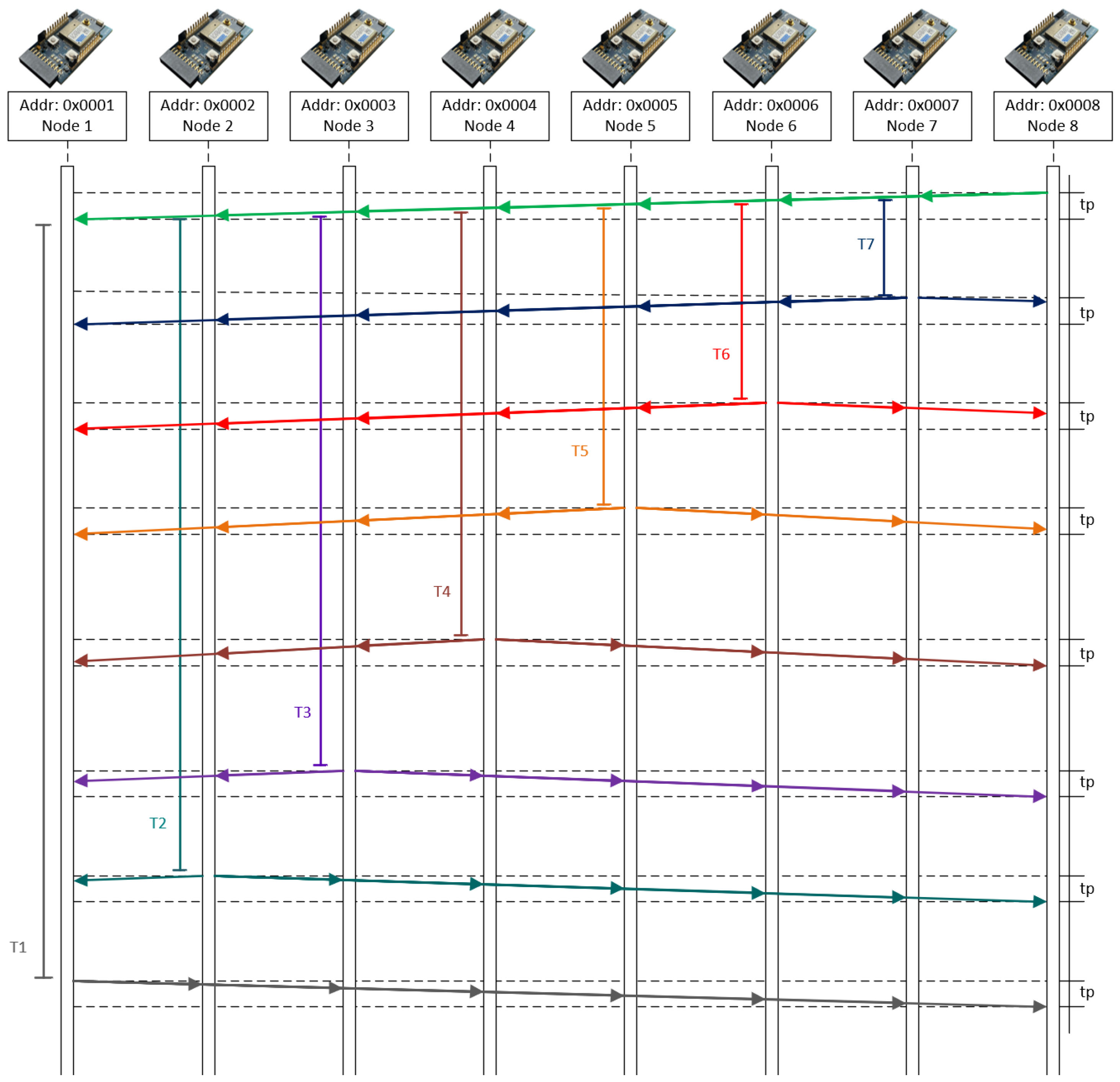
4.4. Transmission Time Measurement

For the measurement of transmission times, the processing time of each node is neglected. The sniffer allows you to display the transmission time in milliseconds; the values obtained do not have decimals.

4.4.1. Measurement of Times Corresponding to the First Test with the Kruskal Algorithm

Different times are obtained when measuring each node’s transmission times by configuring a default route generated by the Kruskal algorithm, as indicated in Figure 19. The diagram illustrates that frames from nodes 6 and 7 require approximately 30 msec to reach the controller, whereas the frame from node 1 takes 18 msec for the same journey. Nodes 5 and 7 are the fastest to reach the controller by not making additional hops. The frames passing through node 1 describe a similar graph until they reach the controller node.

4.4.2. Measurement of Times Corresponding to the Second Test with the Kruskal Algorithm

In this test, a default route generated by the Kruskal algorithm was configured, and higher battery levels were assigned to nodes 3 and 4 compared to the other nodes. Now, it is observed that the frame sent by node 1 needs 24 ms to reach the controller, which implies 6 ms less than in the previous test carried out with the Kruskal algorithm; in this case, the frame sent by node 3 is delayed 6 ms. All frames generated by the other nodes must pass through node 3, causing the last few hops to describe a similar graph for all nodes, as shown in Figure 20. Nodes 4 and 6 generate frames that take 12 ms to reach the controller; the frames of nodes 2, 5, and 7 take 18 ms.

4.4.3. Measurement of Times Corresponding to the First Test with Dijkstra’s Algorithm

By measuring the transmission times of each node when a default route generated by the Dijkstra algorithm was configured, the times indicated in Figure 21 are obtained. The sequence diagram reveals a uniform duration for frames from all nodes to reach the controller, indicating a scenario where frames are directly sent to the controller.

4.4.4. Measurement of Times Corresponding to the Second Test with Dijkstra’s Algorithm

The same results are obtained by configuring a default route generated by the Dijkstra algorithm, with nodes 3 and 4 having higher battery levels than the others, as shown in Figure 22. No changes in transmission times are observed due to the battery levels of the mentioned nodes.

4.5. Results Comparison

Three tests are evaluated, the two previous ones and one additional one, in which nodes 7 and 8 have a higher voltage level. The time it takes for a frame generated by a node to reach the controlling node was analyzed. In the column diagrams in Figure 23, you can see how the sending time of a frame varies when no algorithm is applied, when the Kruskal algorithm is used, and when the Dijkstra algorithm is applied. In all the tests, it is evident that the sending time from node 1 to node 7 decreases when no algorithm is applied, and the communication between the nodes and the controller is carried out using the initial default route. The decrease in time is due to the lower number of hops.
In the first test, as seen in Figure 23a, when implementing the Kruskal algorithm, a decrease in time is observed for nodes 1, 2, 3, and 5 compared to when no algorithm is applied. However, the times of nodes 4 and 6 increase considerably. This change is because, in this test, the nodes have similar voltage values, which causes them to send information along a path further away from the controller than the initial path. This increases the number of hops and, therefore, the sending time of a frame. Applying Dijkstra’s algorithm shows a decrease in the sending time for all nodes, except node 7, compared to the times obtained without applying any algorithm. When comparing these times with those obtained using the Kruskal algorithm, it is observed that lower or similar values are obtained. For node 7, it is noted that the sending time is identical in the three cases because this node is the closest to the controller and only makes one hop to reach it.
In the second test, as seen in Figure 23b, implementing Kruskal’s algorithm channels the nodes’ traffic to nodes 3 and 4, which have a higher voltage. Because of this, it takes more time for other nodes to send a frame to the controller. Regarding Dijkstra’s algorithm, the results are consistent with the first test.
In the third test, as seen in Figure 23c, node 7 and the controller node have the highest voltage. With the application of the Kruskal algorithm, it is observed that the times used by each node are similar to when no algorithm is applied. As in the previous test, the algorithm directs traffic to the nodes with the highest voltage. In this case, almost all generated frames must pass through node 7, closest to the controller. In this test, when using the Dijkstra algorithm, the same time values are observed as in the previous tests. In general, this algorithm provides the best results because, in most cases, the nodes require less time to send a frame to the controller.
Finally, the sum of the transmission times of each node is made, obtained in each test and with each algorithm. In this way, it can be analyzed more precisely if there is a decrease in transmission time with the application of each algorithm. Figure 23d shows how implementing both algorithms reduces the total sending time. In general terms, it stands out that the algorithm that yields the best results is Dijkstra’s because it presents lower sending times individually, node by node, and as a whole. This is because, in this scenario, the nodes communicate directly with the controller, so the delay time is the same.
In addition to evaluating the sending time, comparisons are made regarding the number of hops a frame takes to reach the controller. This hop count is carried out for the three tests reviewed previously, as shown in Figure 24. When the Kruskal algorithm is implemented in the first test, as shown in Figure 24a, it is observed that nodes 4 and 6 present the most significant number of hops, with similar values between them. In contrast, nodes 5 and 7 make only one hop to reach the controller. Applying Dijkstra’s algorithm in this test results in all nodes needing a single hop to reach the controller. The same results are obtained in the following tests, similar to what was observed in the time measurement.
In the second test, as shown in Figure 24b, with the use of Kruskal’s algorithm, it is noted that nodes 2, 5, and 7 have the same number of hops. The other nodes show similar values, but node 3 performs only one jump, which is explained by the higher voltage levels in nodes 3 and 4.
In the third test (as shown in Figure 24c), a graph similar to the graph without the algorithm is observed when applying the Kruskal algorithm. The hops decrease as the nodes closest to the controller are considered. Furthermore, it is highlighted that node 7 makes a single hop in all three cases.
Figure 24d compares the sum of jumps obtained in each test. It can be seen that in all tests, a smaller number of jumps is achieved when applying both algorithms. It is also relevant to mention that, in the second test, when applying the Kruskal algorithm, a decrease in the number of hops is observed, even though the sending time remained constant when no algorithm was used.
In summary, based on the results evidenced in each of the tests and even though both algorithms generate a reduction in sending times and the number of hops, it can be stated that Dijkstra’s algorithm presents better results. This is because both the frame sending time per node and the number of hops decreases significantly with their application.

5. Conclusions

In conclusion, this paper addresses the challenges associated with applying software-defined networking (SDN) technology to wireless sensor networks (WSNs) with nodes operating on limited computing capabilities and battery power.
Minimizing energy consumption, arising from processing at the network layer and delays in routing algorithm execution at nodes, necessitates the adoption of SDN technology in WSNs. Our proposal uses the concept of SDN, but for transmitting information between the controller and the sensor nodes, the IEEE 802.15.4 protocol is used instead of the network protocols used in WSNs. The controller assesses the WSN network to determine the optimal topology, considering both the battery and signal levels upon frame reception to designate the relay node. The received signal level is linked to transmission errors caused by channel noise and the distance at the time of transmission power. To validate our proposal, we implemented a prototype built for this purpose and the Dijkstra and Kruskal algorithm to determine the most optimal topology for the network.
Algorithms are presented so that the nodes can send their information to the gateway and so that the gateway sends the information to the WSN nodes operating with IEEE 802.15.4. With the results obtained, the advantage of using a controller for determining the network topology has been demonstrated, eliminating the implementation of a routing algorithm in the nodes. Using the link protocol instead of routing protocols has been validated, thereby reducing processing and transmission delays in the data. The results obtained allow us to continue developing an architecture for SDWSN.
The key features of this work include the utilization of an SDN-enabled controller to reduce processing delays, the incorporation of node battery levels and distance considerations in route selection, the adoption of the IEEE 802.15.4 protocol for data transport, and the proposal of an SDWSN architecture without network-level protocols.

Author Contributions

Conceptualization, C.E.A., L.C. and C.T.; methodology, C.E.A., L.C., C.T. and J.C.-R.; software, C.E.A. and L.C.; validation, C.E.A., L.C., C.T. and J.C.-R.; formal analysis, C.E.A., L.C., C.T. and J.C.-R.; investigation, C.E.A., L.C., C.T. and J.C.-R.; resources, C.E.A., C.T. and J.C.-R.; data curation, C.E.A., L.C. and C.T.; writing—original draft preparation, C.E.A., L.C., C.T. and J.C.-R.; writing—review and editing, C.E.A., L.C., C.T. and J.C.-R.; visualization, C.E.A., L.C., C.T. and J.C.-R.; supervision, C.E.A., L.C., C.T. and J.C.-R.; project administration, C.E.A. and C.T.; funding acquisition, C.E.A. and C.T. All authors have read and agreed to the published version of the manuscript.

Funding

Escuela Politécnica Nacional has supported this work through project PIIF-21-04.

Institutional Review Board Statement

Not applicable.

Informed Consent Statement

Not applicable.

Data Availability Statement

Data are contained within the article.

Acknowledgments

Jorge Carvajal-Rodriguez acknowledges the support provided by the Escuela Politécnica Nacional for performing doctoral studies.

Conflicts of Interest

The authors declare no conflicts of interest.

References

  1. Sisinni, E.; Saifullah, A.; Han, S.; Jennehag, U.; Gidlund, M. Industrial Internet of Things: Challenges, Opportunities, and Directions. IEEE Trans. Ind. Inform. 2018, 14, 4724–4734. [Google Scholar] [CrossRef]
  2. Ali, A.; Ming, Y.; Chakraborty, S.; Iram, S. A Comprehensive Survey on Real-Time Applications of WSN. Future Internet 2017, 9, 77. [Google Scholar] [CrossRef]
  3. Borges, L.M.; Velez, F.J.; Lebres, A.S. Survey on the Characterization and Classification of Wireless Sensor Network Applications. IEEE Commun. Surv. Tutor. 2014, 16, 1860–1890. [Google Scholar] [CrossRef]
  4. Fabbri, F.; Buratti, C.; Verdone, R. A Multi-Sink Multi-Hop Wireless Sensor Network Over a Square Region: Connectivity and Energy Consumption Issues. In Proceedings of the 2008 IEEE Globecom Workshops, New Orleans, LA, USA, 30 November–4 December 2008; pp. 1–6. [Google Scholar] [CrossRef]
  5. Kreutz, D.; Ramos, F.M.V.; Veríssimo, P.E.; Rothenberg, C.E.; Azodolmolky, S.; Uhlig, S. Software-Defined Networking: A Comprehensive Survey. Proc. IEEE 2015, 103, 14–76. [Google Scholar] [CrossRef]
  6. Modieginyane, K.M.; Letswamotse, B.B.; Malekian, R.; Abu-Mahfouz, A.M. Software defined wireless sensor networks application opportunities for efficient network management: A survey. Comput. Electr. Eng. 2018, 66, 274–287. [Google Scholar] [CrossRef]
  7. Acosta, C.E.; Gil-Castineira, F.; Costa-Montenegro, E.; Silva, J.S. Reliable Link Level Routing Algorithm in Pipeline Monitoring Using Implicit Acknowledgements. Sensors 2021, 21, 968. [Google Scholar] [CrossRef] [PubMed]
  8. Acosta, C.E.; Cali, D.; Espinosa, C. Autoconfiguration with Global Addresses Using IEEE 802.15.4 Standard in Multi-hop Networks. Enfoque UTE 2021, 12, 44–58. [Google Scholar] [CrossRef]
  9. Singh, P.K.; Paprzycki, M. Introduction on Wireless Sensor Networks Issues and Challenges in Current Era. In Handbook of Wireless Sensor Networks: Issues and Challenges in Current Scenario’s; Singh, P.K., Bhargava, B.K., Paprzycki, M., Kaushal, N.C., Hong, W.C., Eds.; Advances in Intelligent Systems and Computing; Springer International Publishing: Cham, Switzerland, 2020; pp. 3–12. [Google Scholar] [CrossRef]
  10. Kumar, S.A.A.; Ovsthus, K.; Kristensen, L.M. An Industrial Perspective on Wireless Sensor Networks—A Survey of Requirements, Protocols, and Challenges. IEEE Commun. Surv. Tutor. 2014, 16, 1391–1412. [Google Scholar] [CrossRef]
  11. Lai, X.; Ji, X.; Zhou, X.; Chen, L. Energy Efficient Link-Delay Aware Routing in Wireless Sensor Networks. IEEE Sens. J. 2018, 18, 837–848. [Google Scholar] [CrossRef]
  12. Ma, X.; Luo, W. The Analysis of 6LowPAN Technology. In Proceedings of the 2008 IEEE Pacific-Asia Workshop on Computational Intelligence and Industrial Application, Wuhan, China, 19–20 December 2008; Volume 1, pp. 963–966. [Google Scholar] [CrossRef]
  13. Javaid, A. Understanding Dijkstra’s Algorithm. Available at SSRN 2340905. 2013. Available online: https://papers.ssrn.com/sol3/papers.cfm?abstract_id=2340905 (accessed on 1 December 2023).
  14. Guttoski, P.B.; Sunye, M.S.; Silva, F. Kruskal’s Algorithm for Query Tree Optimization. In Proceedings of the 11th International Database Engineering and Applications Symposium (IDEAS 2007), Banff, AB, Canada, 6–8 September 2007; pp. 296–302. [Google Scholar] [CrossRef]
  15. Al-Karaki, J.; Kamal, A. Routing techniques in wireless sensor networks: A survey. IEEE Wirel. Commun. 2004, 11, 6–28. [Google Scholar] [CrossRef]
  16. Pedditi, R.B.; Debasis, K. Energy Efficient Routing Protocol for an IoT-Based WSN System to Detect Forest Fires. Appl. Sci. 2023, 13, 3026. [Google Scholar] [CrossRef]
  17. Tyagi, V.; Singh, S. Network resource management mechanisms in SDN enabled WSNs: A comprehensive review. Comput. Sci. Rev. 2023, 49, 100569. [Google Scholar] [CrossRef]
  18. Cui, X.; Huang, X.; Ma, Y.; Meng, Q. A Load Balancing Routing Mechanism Based on SDWSN in Smart City. Electronics 2019, 8, 273. [Google Scholar] [CrossRef]
  19. Orozco-Santos, F.; Sempere-Payá, V.; Albero-Albero, T.; Silvestre-Blanes, J. Enhancing SDN WISE with Slicing Over TSCH. Sensors 2021, 21, 1075. [Google Scholar] [CrossRef] [PubMed]
  20. Younus, M.U.; Khan, M.K.; Bhatti, A.R. Improving the Software-Defined Wireless Sensor Networks Routing Performance Using Reinforcement Learning. IEEE Internet Things J. 2022, 9, 3495–3508. [Google Scholar] [CrossRef]
  21. Jlassi, W.; Haddad, R.; Bouallegue, R.; Shubair, R. A Combination of Kruskal and K-means Algorithms for Network Lifetime Extension in Wireless Sensor Networks. In Proceedings of the 2021 International Wireless Communications and Mobile Computing (IWCMC), Harbin City, China, 28 June–2 July 2021; pp. 658–663. [Google Scholar] [CrossRef]
  22. Duy Tan, N.; Nguyen, D.N.; Hoang, H.N.; Le, T.T.H. EEGT: Energy Efficient Grid-Based Routing Protocol in Wireless Sensor Networks for IoT Applications. Computers 2023, 12, 103. [Google Scholar] [CrossRef]
  23. Fazio, M.; Buzachis, A.; Galletta, A.; Celesti, A.; Wan, J.; Longo, A.; Villari, M. A Map-Reduce Approach for the Dijkstra Algorithm in SDN Over Osmotic Computing Systems. Int. J. Parallel Program. 2021, 49, 347–375. [Google Scholar] [CrossRef]
  24. Zhao, J.; Pang, L.; Li, H.; Wang, Z. A Safety-Enhanced Dijkstra Routing Algorithm via SDN Framework. In Proceedings of the 2020 IEEE Fifth International Conference on Data Science in Cyberspace (DSC), Hong Kong, China, 27–30 July 2020; pp. 388–393. [Google Scholar] [CrossRef]
  25. Abderrahim, M.; Hakim, H.; Boujemaa, H.; Touati, F. A Clustering Routing based on Dijkstra Algorithm for WSNs. In Proceedings of the 2019 19th International Conference on Sciences and Techniques of Automatic Control and Computer Engineering (STA), Sousse, Tunisia, 24–26 March 2019; pp. 605–610. [Google Scholar] [CrossRef]
  26. Xiang, W.; Wang, N.; Zhou, Y. An Energy-Efficient Routing Algorithm for Software-Defined Wireless Sensor Networks. IEEE Sens. J. 2016, 16, 7393–7400. [Google Scholar] [CrossRef]
  27. da Silva Santos, L.F.; de Mendonca Júnior, F.F.; Dias, K.L. μSDN: An SDN-Based Routing Architecture for Wireless Sensor Networks. In Proceedings of the 2017 VII Brazilian Symposium on Computing Systems Engineering (SBESC), Curitiba, PR, Brazil, 6–10 November 2017; pp. 63–70. [Google Scholar] [CrossRef]
  28. Banerjee, A.; Hussain, D.M.A. SD-EAR: Energy Aware Routing in Software Defined Wireless Sensor Networks. Appl. Sci. 2018, 8, 1013. [Google Scholar] [CrossRef]
  29. Al-Hubaishi, M.; Çeken, C.; Al-Shaikhli, A. A novel energy-aware routing mechanism for SDN-enabled WSAN. Int. J. Commun. Syst. 2019, 32, e3724. [Google Scholar] [CrossRef]
  30. Criollo, L.; Egas, C.; Tipantuña, C.; Carvajal, J. SDN-Enabled Efficient Default Route Configuration in IEEE 802.15.4 Protocol: Repository of Node Configuration. 2024. Available online: https://github.com/criolloluis410/ATZB-256RFR2-Normal-Node-Configuration (accessed on 18 January 2024).
  31. Criollo, L.; Egas, C.; Tipantuña, C.; Carvajal, J. SDN-Enabled Efficient Default Route Configuration in IEEE 802.15.4 Protocol: Repository of Controller. 2024. Available online: https://github.com/criolloluis410/Route-Generator-Aplication (accessed on 18 January 2024).
Figure 1. Network prototype implemented.
Electronics 13 01537 g001
Figure 2. Route generator application with several nodes’ voltage and signal level data.
Electronics 13 01537 g002
Figure 3. Flowchart used in the development of the route generator application.
Electronics 13 01537 g003
Figure 4. SmartRF packett sniffer application.
Electronics 13 01537 g004
Figure 5. Application operation.
Electronics 13 01537 g005
Figure 6. Receiving and sending information within the network prototype.
Electronics 13 01537 g006aElectronics 13 01537 g006b
Figure 7. Example of default routes.
Electronics 13 01537 g007
Figure 8. Communication between nodes and the controller through initial default route (uplink).
Electronics 13 01537 g008
Figure 9. Node delay components.
Electronics 13 01537 g009
Figure 10. Communication between nodes and controller through the downlink.
Electronics 13 01537 g010
Figure 11. Sequence diagram 2: Sending the broadcast frame.
Electronics 13 01537 g011
Figure 12. Data sent from nodes to the controller.
Electronics 13 01537 g012
Figure 13. Execution of the Kruskal algorithm on the prototype.
Electronics 13 01537 g013
Figure 14. Test 1.1: Default route generated by the Kruskal algorithm with nodes having a similar battery level.
Electronics 13 01537 g014
Figure 15. Execution of the Dijkstra algorithm on the prototype.
Electronics 13 01537 g015
Figure 16. Test 1.2: Default route generated by the Dijkstra algorithm where the nodes have a similar battery level.
Electronics 13 01537 g016
Figure 17. Test 2.1: Default route generated by the Kruskal algorithm where nodes three and four have higher battery levels.
Electronics 13 01537 g017
Figure 18. Test 2.2 Default route generated by the Dijkstra algorithm where nodes three and four have higher battery levels.
Electronics 13 01537 g018
Figure 19. Sequence diagram 3: Test 1.1 Default route generated by the Kruskal algorithm with nodes having similar battery levels.
Electronics 13 01537 g019
Figure 20. Sequence diagram 4: Test 2.1 Default route generated by the Kruskal algorithm where nodes three and four have higher battery levels.
Electronics 13 01537 g020
Figure 21. Sequence diagram 5: Test 1.2 Default route generated by the Dijkstra algorithm where the nodes have similar battery levels.
Electronics 13 01537 g021
Figure 22. Sequence diagram 6: Test 2.2 Default route generated by the Dijkstra algorithm where nodes three and four have higher battery levels.
Electronics 13 01537 g022
Figure 23. Comparison of results without using algorithms, the Kruskal algorithm, and the Dijkstra algorithm. (a) Test 1: Time for a frame to reach the controller with nodes with a similar battery level. (b) Test 2: Time for a frame to reach the controller with nodes three and four having higher battery levels. (c) Test 3: Time for a frame to reach the controller with nodes seven and eight having higher battery levels. (d) Time comparison for each test.
Electronics 13 01537 g023
Figure 24. Comparing the number of hops without using algorithms, the Kruskal algorithm, and the Dijkstra algorithm. (a) Test 1: Number of hops to reach the controller with nodes having similar battery levels. (b) Test 2: Number of hops to reach the controller with nodes three and four having higher battery levels. (c) Test 3: Number of hops to reach the controller with nodes seven and eight having higher battery levels. (d) Comparison of hops in each test performed.
Electronics 13 01537 g024
Table 1. Summary of routing works in SDWSN.
RefYearDescriptionNetwork Layer ProtocolLink Layer ProtocolHardware/BitsSimulationImplemented Algortihm
[26]2016Energy-efficient routing algorithm for SDWSNsNot reportedNot reportedNo implementedYesNWPSO
[27]2017 μ -SDN6LowPAN802.15.4ARM920T/32ImplementationAODV, LQRP routing protocols
[28]2018Software-defined energy aware routing SD-EARNot reportedNot reportedNo implementedYesbased on sleep request—sleep grant mechanism
[29]2018SDWSN-architectureNot reportedNot reportedNo implementedYesDijkstra
[25]2019Clustering Routing based on Dijkstra algorithm for WSNsNot reportedNot reportedNo implementedYesDijkstra
[21]2021Kruskal-based SDWSNNot reportedNot reportedNo implementedYesKruskal
[20]2022RL-Based on SDWSNIP802.11,STPRaspberry Pi/64ImplementationKruskal, Dijkstra
Our Work2024Routing proposal for SDWSNNot used802.15.4RCB256RFR2/8NoKruskal, Dijkstra
Disclaimer/Publisher’s Note: The statements, opinions and data contained in all publications are solely those of the individual author(s) and contributor(s) and not of MDPI and/or the editor(s). MDPI and/or the editor(s) disclaim responsibility for any injury to people or property resulting from any ideas, methods, instructions or products referred to in the content.

