Multi-Frequency Noise Reduction Method for Underwater Radiated Noise of Autonomous Underwater Vehicles

Abstract

The multi-frequency noisy vibration of an autonomous underwater vehicle (AUV) is a significant factor affecting the performance of shear probes mounted on the head of AUVs. Many efforts have been made to suppress mechanical radiation noise; however, conventional noise reduction methods have their limitations, such as mode mixing. In order to extract thorough information from the aliasing modes and achieve multi-frequency mode targeted correction, a multi-frequency noise reduction method is proposed, based on secondary decomposition and the multi-mode coherence correction algorithm. Weak impulses in aliasing shear mode are enhanced, and mixing frequencies are isolated for thorough decomposition. Noisy mechanical vibrations in the shear modes are eliminated with the use of the acceleration modes along the identical central frequency series. The denoised modes are used to reconstruct the cleaned shear signal, and the updated spectra are aligned with the standard Nasmyth spectrum. Compared with the raw profiles, the variation in the dissipation rate estimated from the corrected shear is reduced by more than an order of magnitude.

1. Introduction

An autonomous underwater vehicle (AUV) provides mobility and carrying capacity for microstructure probes, making it an ideal platform for underwater applications [1]. Robust and accurate underwater measurements are significant in AUV-based turbulence investigation [2]. However, an AUV in motion has the potential to be a noise source [3]. During navigation, the mechanical structures of the AUV generate multi-frequency variations and radiated noise [4]. This can affect the detection of probes through the hull and decrease the quality of collected data. Therefore, it is crucial to eliminate their multi-frequency self-noise for forthcoming turbulence attribute analysis.

Recently, a lot of noise suppression approaches have been developed to remove disturbing contamination and extract accurate information from raw signals. Basically, there are three types of algorithms that are widely used in noise reduction.

Initially, classical noise reduction algorithms based on time–frequency analysis were used to remove noisy oscillations; some representative methods are short-time Fourier transform analysis (STFT) [5], the wavelet transform method [6,7,8,9,10], and adaptive local iterative filtering (ALIF) [11]. STFT has the ability to extract the fixed time–frequency characteristics from nonlinear data. 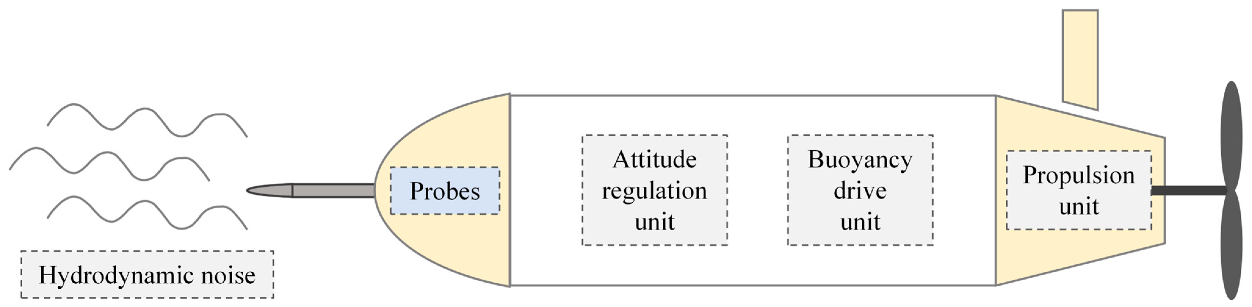It should be noted that the presence of noise is attributed to various sources (Figure 1), including the propulsion unit, the attitude regulation unit, and the buoyancy drive unit [12]. Thus, the noisy vibration observed consists of multi-frequency components that span a wide frequency range and are not limited to a specific frequency. Given the multi-frequency nature of contamination, updated methods have been devised to enhance signal accuracy. Piera [13] developed a time–frequency correction algorithm using a wavelet transform to identify turbulent patches and remove signal noise. Similarly, Suyi [8] presented a wavelet correction technique to suppress oceanic turbulence noise. ALIF decomposes the records into a finite number of stable components, thereby reducing noisy contamination. However, the prior parameters need to be selected according to the signal characteristics, and the performance of these reduction methods is highly dependent on these empirical settings.

A number of noise correction techniques based on decomposition and integration have then been presented, starting with the empirical mode decomposition (EMD) method [14,15,16,17]. Huang [15] introduced a Hilbert–Huang transform that can provide multi-scale information for the denoising procedure and utilize the multiple modes to reconstruct the effective data. The method has been used to successfully remove noise contamination in various fields, including engine signals [14], micro-seismic signals [16], and electrocardiogram signals [17]. It has also been used to improve techniques such as ensemble empirical mode decomposition (EEMD) [18], uniform phase empirical mode decomposition (UPEMD) [19], and modified complete ensemble empirical mode decomposition with adaptive noise (MCEEMDAN) [20]. They obtain the decomposed components through iterative calculation; however, the decomposition in these methods is often lacking in thoroughness, resulting in mode mixing during application. Part of the useful information is hidden in the mixed mode function (MMF), which significantly affects noise correction performance. Furthermore, the corresponding instantaneous frequency and amplitude of modes can only be obtained based on the decomposed variations. In other words, the decomposed modes control the corresponding features. Variational mode decomposition (VMD) [21,22,23] is an adaptive time–frequency domain decomposition method. It decomposes the signal into modes with limited bandwidth, and each component has its specific central frequency. Furthermore, VMD has the advantage for backtracking modes according to the central frequency series [24,25].

In recent years, researchers have explored noise reduction through secondary decomposition to compensate for the limitations of one-time decomposition, which would reduce the noise residue and promote complete decomposition [26,27]. A hybrid noise reduction approach, combining the complete ensemble empirical mode decomposition with adaptive noise (CEEMDAN), the minimum mean square variance criterion (MMSVC), and the least mean square adaptive filter (LMSAF) has been introduced for underwater acoustic signals [28]; it combines the multiple advantages of these methods to suppress mode mixing and provide an appropriate parameter decision. Furthermore, a combined secondary optimization decomposition model has been employed to suppress noisy contamination with the use of amplitude-aware permutation entropy, dynamic interval threshold filtering, and mutual information [29]. In addition, secondary decomposition is in its initial stages of implementation in noise reduction in turbulence signals. It has great advantages in detecting multi-frequency components and ameliorating the quality of records.

Considering the complexity of the turbulence shear signal, the limitations of existing noise reduction approaches should be addressed. Therefore, we propose a novel multi-frequency noise reduction (MFNR) method for turbulence shear signals combined with secondary decomposition and the cross-spectral coherence correction (CSCC) algorithm. The secondary decomposition technique is capable of identifying all relevant multi-frequency peaks and partitioning the raw signal into thorough modes. In addition, when accompanied by vibration modes with equivalent frequency characteristics, the multi-frequency noisy vibration contained in the shear modes can be suppressed. Compared with the traditional noise reduction method, it is verified that it effectively suppresses the multi-frequency noisy contamination induced by vibration and has good performance in ameliorating the data quality of turbulence microstructure shear signals.

The paper is structured as follows: In Section 2, a new noise reduction method combined with secondary decomposition and the multi-mode coherence correction algorithm is presented. In Section 3, the feasibility of this method is demonstrated by using turbulence data obtained from a turbulence microstructure instrument, wave number spectrum characteristics, and dissipation rate variation. The paper concludes in Section 4.

2. Methods

In general, a one-time traditional decomposition method is insufficient to thoroughly decompose the original signal, and effective information may be hidden in the aliasing modes. Accordingly, aliasing modes would lead to the incomplete reduction in the multi-frequency noisy contamination and affect the measurement quality for turbulence analysis. As a result, a multi-frequency noise reduction (MFNR) method based on secondary decomposition and the CSCC algorithm has been developed. The overview of the proposed MFNR method is shown in Figure 2. The proposed reduction methodology consists of first decomposition, secondary decomposition, constrained decomposition, and multi-mode coherence correction.

2.1. First Decomposition

The original shear signal is composed of multi-frequency variations, and multiple mode decomposition methods are generally used to separate and extract the multi-frequency features contained in the original data. Since the variational mode decomposition (VMD) method provides a way to adaptively decompose a signal into modes with different central frequencies, we chose to use it for the preliminary decomposition of the raw shear signal ($s\left(t\right)$).

In order to separate the raw shear signal ($s\left(t\right)$) into original modes by using the VMD algorithm, the widths of the decomposed modes (${su}_k\left(t\right)$) are required to be minimized, and the sum of the modes $({su}_k\left(t\right)$) is required to be equal to the original signal ($s\left(t\right)$). Further, the constrained variational problem in the decomposition procedure is given as

$$\left\{\begin{array}{c}\underset{\left\{u_k\right\},\left\{{\omega }_k\right\}}{\min }\left\{{\displaystyle \sum _k}{‖{\partial }_t\left[\left(\delta \left(t\right)+\frac{j}{\pi t}\right)u_k\left(t\right)\right]exp\left(-j{\omega }_{k}t\right)‖}_2^2\right\},\\ s.t.{\displaystyle \sum _k}{su}_k=s\left(t\right)\end{array}\right.$$

(1)

where ${su}_k\left(t\right)$ represents the decomposed components and ${\omega }_k$ represents the original central frequency of the mode. Subsequently, it is transformed into an unconstrained variational problem with the utilization of a quadratic penalty factor ($\alpha$) and the Lagrange operator ($\mathsf{\lambda }$).

By using the alternating direction multipliers, the original shear modes (${su}_k$), the original central frequency (${\omega }_k$), and the Lagrange operator ($\mathsf{\lambda }$) are iterated to obtain the corresponding optimal solution:

$${su}_k^{n+1}\left(\omega \right)=\frac{s\left(\omega \right)-\sum _{i\ne k}{su}_i\left(\omega \right)+\frac{\mathsf{\lambda }\left(\omega \right)}{2}}{1+2\alpha {\left(\omega -{\omega }_k\right)}^2}$$

(2)

$${\omega }_k^{n+1}=\frac{{\int }_0^{\mathrm{\infty }}\omega {\left|u_k\left(\omega \right)\right|}^{2}d\omega }{{\int }_0^{\mathrm{\infty }}{\left|u_k\left(\omega \right)\right|}^{2}d\omega }$$

(3)

$${\lambda }^{n+1}\left(\omega \right)\leftarrow {\lambda }^n\left(\omega \right)+\tau \left[s\left(\omega \right)-\sum _k{su}_k^{n+1}\left(\omega \right)\right]$$

(4)

${su}_k$, ${\omega }_k$, and $\mathsf{\lambda }$ are iteratively updated until $\sum _k{‖{\widehat{su}}_k^{n+1}-{\widehat{su}}_k^n‖}_2^2/{‖{\widehat{su}}_k^n‖}_2^2<\tau$ is satisfied.

In general, overdecomposition leads to computational redundancy and the over-refinement of signal variation information. Therefore, energy entropy ($E$) [23] is introduced to determine the optimal number of decomposed components ($n$) which guarantees efficient decomposition and information preservation. Energy entropy is expressed as

$$E=-\sum _{i=1}^n{p}_i\log p_i$$

(5)

where $p_i=e_i/e$ is the energy weight, $\left[e_1,e_2,\cdots ,e_n\right]$ is the energy of each mode, and $e$ represents the total energy of the raw signal. It is assumed that the higher the energy entropy, the lower the proportion of mode energy, and vice versa. The optimal number of decomposed modes is determined by the energy entropy sequence. When the original signal is decomposed into $n$ and $n+1$ modes, we can evaluate their corresponding energy entropy, $E_n$ and $E_{n+1}$, respectively. If $E_{n+1}$ is different from $E_n$, it means that the $n$ decomposition is incomplete. On the contrary, if $E_{n+1}$ is similar to $E_n$, it means that $n+1$ modes have been overdecomposed, containing illusive components.

2.2. Secondary Decomposition

Based on the above operation, the original shear modes (${su}_k=\left\{{su}_1,\cdots ,{su}_{n-1},{su}_m\right\}$) and the original central frequency (${\omega }_k=\left\{{\omega }_1,\cdots ,{\omega }_{n-1},{\omega }_m\right\}$) can be obtained, but it should be noted that the one-time decomposition using the VMD method usually lacks thoroughness and leads to mode mixing [29] and multi-frequency variation fusion, which impede efficient noise reduction. Therefore, we introduce secondary decomposition to thoroughly extract the multi-frequency residue from the mixed mode function (MMF).

Prior to the secondary decomposition, an attempt should be made to distinguish the MMF and the organized mode function (OMF). Here, kurtosis ($k$) [9] is utilized to differentiate the MMF and OMF from the original mode sequences, given as $k={\sum }_{i=1}^N\left(x_i-\mu \right)/N{\delta }^4$. Typically, an OMF, e.g., ${su}_k=\left\{{su}_1,\cdots ,{su}_{n-1}\right\}$, has a relatively organized frequency, and its $k$ value is relatively small. Conversely, an MMF, e.g., ${su}_k=\left\{{su}_m\right\}$, contains significant interfering frequencies, and its corresponding $k$ value is relatively high.

Taking into account the residual components, the demodulation method is utilized to extract the residual frequency mixed in the mode. Since the multiresolution Teager energy operator (MTEO) is sensitive to vibration characteristics and has high temporal resolution for concentrated vibrations at short intervals [30,31], we opted to utilize it for the residual frequency demodulation of the MMF. The equation of discrete-time demodulation is expressed as follows [21]:

$$\mathsf{\psi }\left({su}_p\left(n\right)\right)={\left({su}_p\left(n\right)\right)}^2-{su}_p\left(n-p\right){su}_p\left(n+p\right)$$

(6)

where $\mathsf{\psi }\left[·\right]$ is the demodulation transform operator and $p$ represents the multiresolution parameter. The differentiation operator ($D_p$), the integration operator ($I_p$), and the composite operator (${∆}_p$) are defined to enhance noisy vibration.

$$D_p\left({su}_p\left(n\right)\right)=\left({su}_p\left(n\right)-{su}_p\left(n-1\right)\right)-\cdots -\left({su}_p\left(n-p+1\right)-{su}_p\left(n-p\right)\right)$$

(7)

$$I_p\left({su}_p\left(n\right)\right)=\left({su}_p\left(n\right)+{su}_p\left(n-1\right)\right)-\cdots -\left({su}_p\left(n-p+1\right)+{su}_p\left(n-p\right)\right)$$

(8)

$${∆}_p\left({su}_p\left(n\right)\right)=D_{p-1}\left(I_1\left(\left({su}_p\left(n\right)\right)\right)\right)=I_{p-1}\left(D_1\left(\left({su}_p\left(n\right)\right)\right)\right)={su}_p\left(n\right)-{su}_p\left(n-p\right)$$

(9)

Thus, Equation (6) can be obtained as follows:

$${\mathsf{\psi }}_p\left({su}_p\left(n\right)\right)={\left({∆}_p\left({su}_p\left(n\right)\right)\right)}^2-{su}_p\left(n\right)·{∆}_p\left({∆}_p\left({su}_p\left(n\right)\right)\right)$$

(10)

where ${∆}_p\left({∆}_p\left({su}_p\left(n\right)\right)\right)={su}_p\left(n\right)-2{su}_p\left(n-p\right)-{su}_p\left(n-2p\right)$.

According to the above procedures, frequencies mixed in the MMF are extracted. Here, $\left\{{\omega }_n,\cdots ,{\omega }_K\right\}$ refers to the central frequency series that is demodulated from the MMF ${su}_k=\left\{{su}_m\right\}$ but ignored. This sequence is appended to the original organized frequency series. That is, the original central frequency series, ${\omega }_k=\left\{{\omega }_1,\cdots ,{\omega }_{n-1},{\omega }_m\right\}$, is updated to ${\omega }_k=\left\{{\omega }_1,\cdots ,{\omega }_{n-1},{\omega }_n,\cdots ,{\omega }_K\right\}$. Similarly, the residual components mixed in the MMF ${su}_k=\left\{{su}_m\right\}$ are extracted into isolated new modes, e.g., ${su}_k=\left\{{su}_n,\cdots ,{su}_K\right\}$. That is, according to the specific central frequency series, the original shear modes, ${su}_k=\left\{{su}_1,\cdots ,{su}_{n-1},{su}_m\right\}$, are updated to ${su}_k=\left\{{su}_1,\cdots ,{su}_{n-1},{su}_n,\cdots ,{su}_K\right\}$ by secondary VMD. Based on the secondary decomposition procedure, the complete central frequency and the multi-frequency components can be thoroughly separated.

2.3. Constrained Decomposition

As mentioned above, raw shear data are thoroughly decomposed into a complete mode sequence, ${su}_k=\left\{{su}_1,\cdots ,{su}_{n-1},{su}_n,\cdots ,{su}_K\right\}$, and provide an identical central frequency series, ${\omega }_k=\left\{{\omega }_1,\cdots ,{\omega }_{n-1},{\omega }_n,\cdots ,{\omega }_K\right\}$. Therefore, based on the specific central frequency series, the vibration signal ($a\left(t\right)$) can be decomposed into complete modes ${au}_k=\left\{{au}_1,\cdots ,{au}_{n-1},{au}_n,\cdots ,{au}_K\right\}$ by using the VMD algorithm once.

2.4. Multi-Mode Coherence Correction

The measured shear signal is assumed to be correlated with the pure shear data and vibration contamination [32,33,34]. The conventional CSCC algorithm would directly remove coherent variation induced by vibration. However, it would mask noise contamination caused by low-frequency vibration, as high-frequency vibration is too prominent. Therefore, multi-mode coherence correction is improved based on the conventional CSCC method to effectively suppress multi-frequency vibration.

Similarly, a raw shear mode is considered to be a combination of a pure shear component and a vibration component with identical central frequency. To improve data quality, the useless components need to be suppressed, leaving the useful component for effective data reconstruction. With the accompaniment of vibration modes sharing an identical frequency band, the noisy contamination contained in the shear modes can be thoroughly removed. The reduction equation can be expressed as follows:

$${su}_k\left(t\right)={\widehat{su}}_k\left(t\right)+b\mathrm{\ast }{au}_k\left(t\right)$$

(11)

where ${su}_k\left(t\right)$ represents the raw shear modes, ${au}_k\left(t\right)$ represents the vibration mode of identical central frequency, the caret ${\widehat{su}}_k\left(t\right)$ denotes the pure shear mode in fluid flow, and $\mathrm{\ast }$ is the convolution. Moreover, $b$ represents the influence of vibration exerted on the shear mode and the weight coefficient, and it is given as $b^2={\varphi }_{sa}\left(\omega \right){\varphi }_{sa}^{\mathrm{*}}\left(\omega \right)/{\varphi }_{ss}\left(\omega \right){\varphi }_{aa}\left(\omega \right)$. ${\varphi }_{sa}\left(\omega \right)$ is the cross-correlation spectrum of the shear mode and acceleration mode, ${\varphi }_{ss}\left(\omega \right)$ represents the auto-correlation spectrum of the shear mode, and ${\varphi }_{aa}\left(\omega \right)$ represents the auto-correlation spectrum of the acceleration mode.

Subsequently, the noise induced by multi-frequency vibration is suppressed in each shear mode. We denoise the shear modes and restructure them to obtain the cleaned signal, $\widehat{s}\left(t\right)$.

3. Results

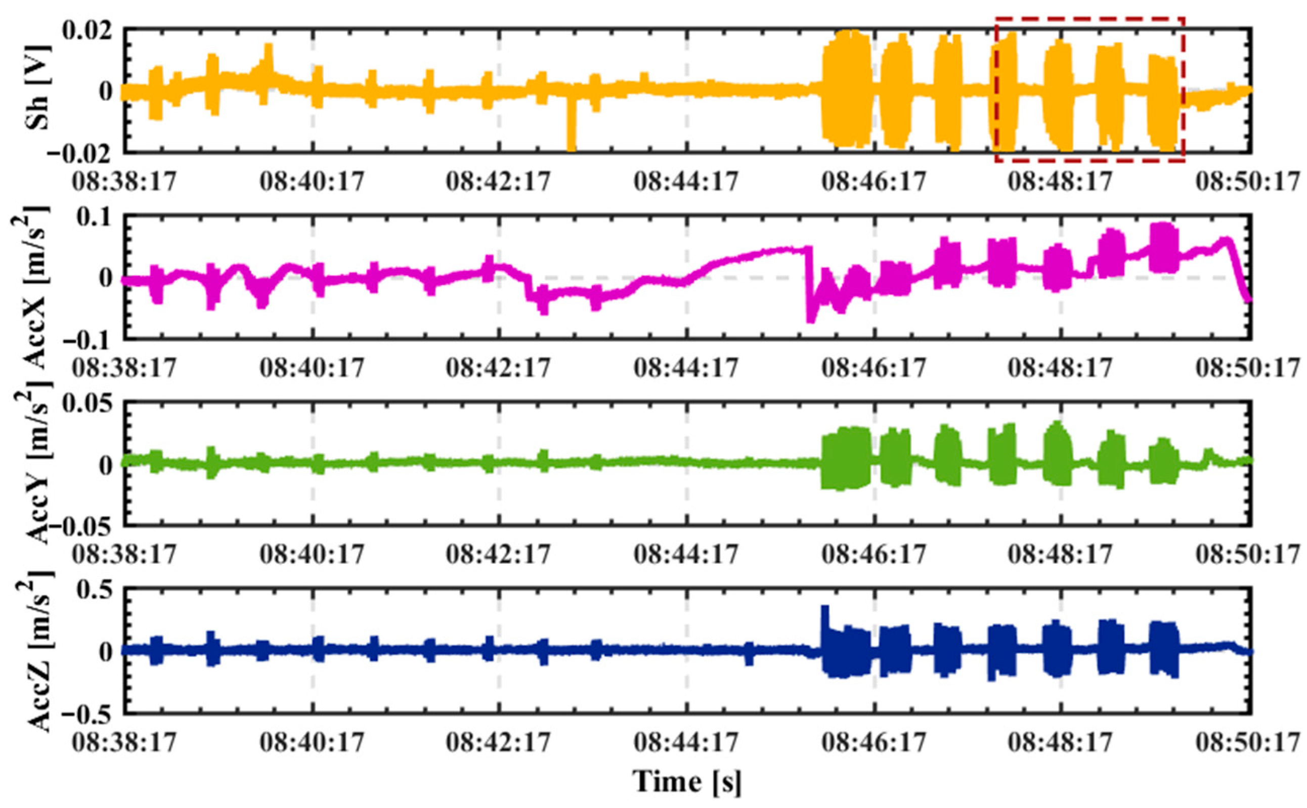
Here, we present experiments demonstrating the effectiveness of noise reduction by using the proposed MFNR algorithm. An autonomous underwater vehicle (AUV) (Figure 3) was deployed in Thousand Lake (with an average water depth of 30 m) on 18 July 2020. We measured the time series of shear and acceleration by using an AUV equipped with a shear probe and a three-directional acceleration probe at a sampling rate of 1024 Hz. Three navigation patterns were recorded: the diving stage, the horizontal navigation stage, and the upward-floating stage. The unprocessed shear variation (upper panel in Figure 4) was contaminated by multiple sources of vibration, as indicated by the acceleration variations (bottom three panels). Therefore, the proposed MFNR method was used to eliminate the vibration interference.

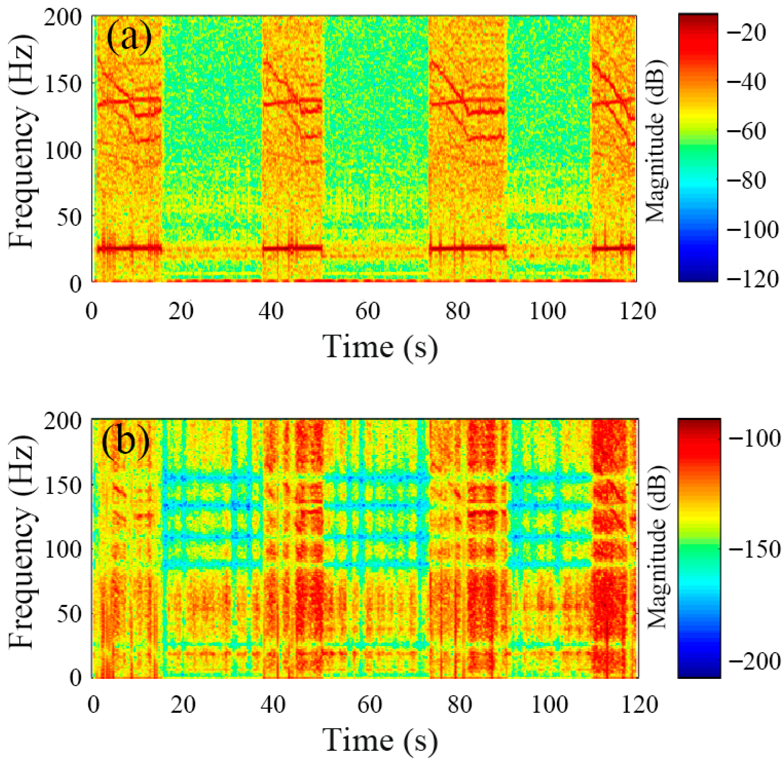
The shear data were sampled over 120 s (red rectangle in Figure 4) to differentiate the overlapping characteristic frequencies from a total of 204 min of records. The frequency spectrum of original shear data (black line in Figure 5b) showed only the clear recognition of 25 Hz. However, other vibration frequencies, previously observed in experiments, could not be easily identified and distinguished. As a result, the proposed algorithm was implemented to extract these mixed frequencies. The optimal number of separated modes for the first decomposition procedure was determined by using energy entropy. The number of separated modes was iteratively increased, and we evaluated the corresponding energy entropy variation of each mode at each decomposition step. When we decomposed the original shear signal into six modes, we discovered that they had energy entropy values that were extremely similar to those found when they were decomposed into five modes (see

Table 1. The energy entropy variation.

Decomposition Number	Energy Entropy
	${\mathit{E}}_1$	${\mathit{E}}_2$	${\mathit{E}}_3$	${\mathit{E}}_4$	${\mathit{E}}_5$	${\mathit{E}}_6$
2	0.3037	0.1573
3	0.3032	0.1567	0.0015
4	0.2667	0.3515	0.3045	0.0013
5	0.2665	0.3508	0.3042	0.1887	0.0013
6	0.2661	0.3508	0.3042	0.1867	0.0013	0.0011

). That is, when the original signal was decomposed into six modes, it was overdecomposed, and there were illusive components in these decomposed modes.

Consequently, the optimal number of modes to decompose the signal into was five, and the shear signal was decomposed into five modes in the first decomposition procedure. Figure 5a presents the decomposition of the five shear modes. Figure 5b displays the frequency spectrum of the corresponding mode components. It is clear that only $\left\{{su}_1,{su}_5\right\}$ were successively isolated, while $\left\{{su}_2,{su}_3,{su}_4\right\}$ were modes mixed at 25 Hz. Therefore, the vibration features contained in $\left\{{su}_2,{su}_3,{su}_4\right\}$ were unclear for the denoising process due to this significantly mixed frequency. Then, the $k$ criterion was required to differentiate the MMF from the ambiguous modes, and we applied the MTEO to it to separate these mixed frequencies. The corresponding $k$ curve of the modes is depicted in Figure 6. ${su}_5$ had the highest $k$ value, yet its central frequency exceeded 150 Hz, posing a considerable deviation from the cut-off frequency. Therefore, the MMF was identified as the ${su}_3$ with the highest $k$ value in the lower frequency range. The MTEO demodulation method was then applied to suppress strong disturbances and enhance weak impulses.

The above procedures effectively extracted the hidden frequencies from the residual mode. A comparison of the original time–frequency spectrum and the demodulating time–frequency spectrum is shown in Figure 7. The multi-frequency variations were mixed in the original shear variation, so we could not directly distinguish all of these hidden variations based on the time–frequency spectrum (Figure 7a), except for these extremely obvious variations, such as the 4 Hz and 25 Hz variations (red lines at the bottom of Figure 7a). However, these multi-frequency mixing variations could be thoroughly extracted by using the secondary decomposition procedure. Figure 7b shows the central frequency series that was completely isolated. The original central frequency series was updated to ${\omega }_k=\left[4,25,90,110,130\right]$, which represents the total information mixed in the shear signal. Based on the updated central frequency series, the shear and vibration modes with identical frequencies were then backtracked and constructed. Figure 8 shows the backtracked shear modes and their corresponding frequency spectra. All mixing modes were successively isolated to promote the following denoising procedure, which suppressed multi-frequency vibration contamination.

The raw shear mode is assumed to be correlated with the pure shear component and coherent noise induced by vibration. Thus, multi-mode coherence correction was applied to each pair of shear and acceleration modes to eliminate the vibration-induced inference contained in each shear mode. The original shear modes (black solid curves), the cleaned shear modes (green, purple, and blue solid lines), and the acceleration modes (gray dotted lines) are shown in Figure 9. For simplicity, only the first three modes and their outcomes are presented. The original shear mode peaks induced by variation are clearly suppressed in the corresponding cleaned shear modes.

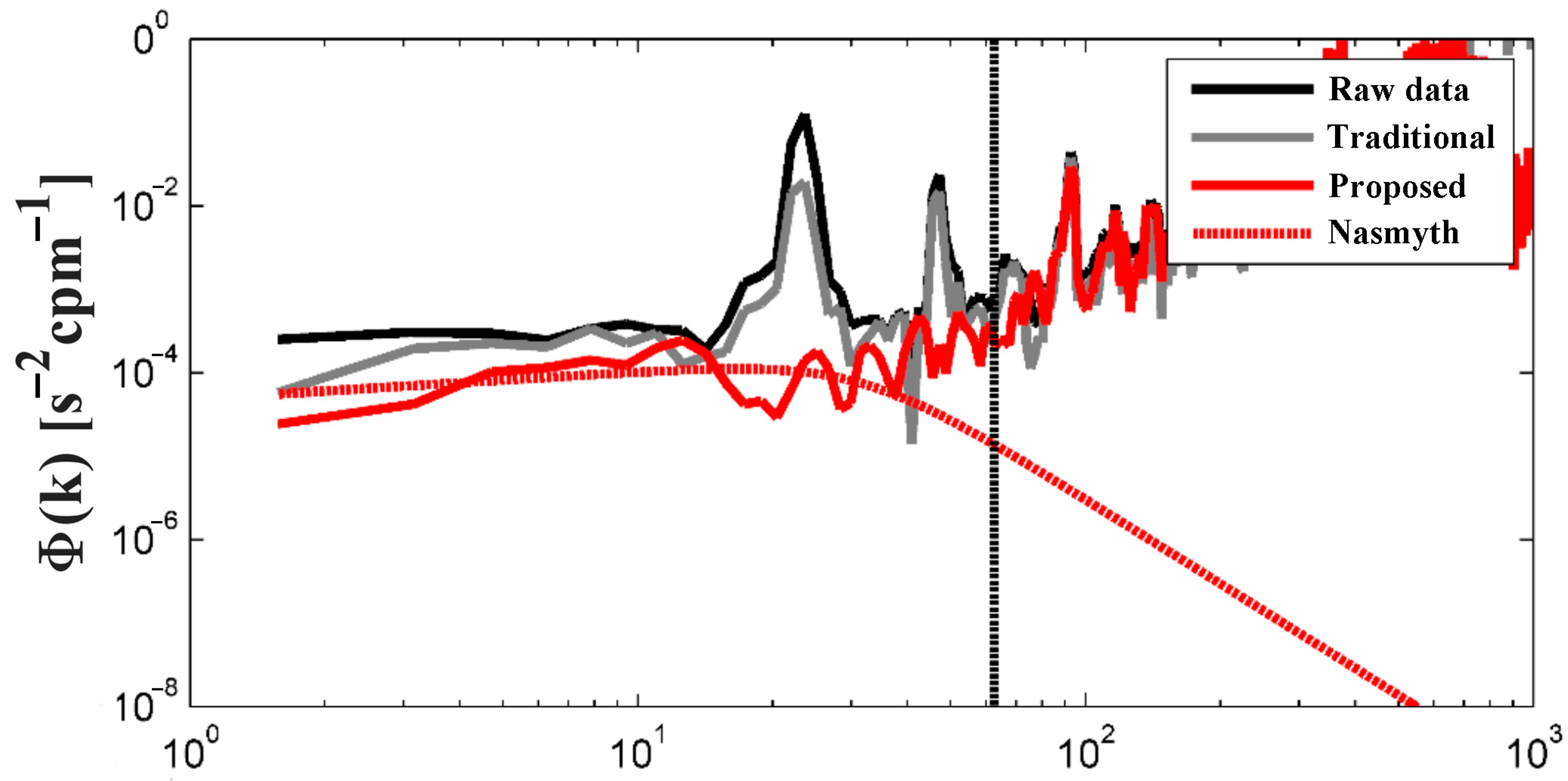
Subsequently, these cleaned modes were reconstructed to examine the turbulence characteristics. Assuming Taylor’s frozen hypothesis [35], the dissipation rate of turbulent kinetic energy is a crucial parameter for scrutinizing the turbulence properties [36]. Furthermore, the Nasmyth spectrum is assumed as a standard criterion for evaluating shear spectra [37].

Figure 10 shows the raw shear spectrum and the cleaned shear spectra processed by using both the proposed MFNR method and the exclusive CSCC algorithm. It is important to note that the raw shear spectrum (represented by the solid black line) exhibits two distinct peaks caused by vibration. These peaks cannot be effectively eliminated through the exclusive utilization of the CSCC algorithm. While the peak at 25 Hz shows some slight attenuation, the peak around 50 Hz remains unchanged. On the contrary, the proposed MFNR method could effectively remove the two prominent peaks, as shown in the cleaned spectrum. The corrected spectrum obtained by the proposed method closely matched the standard Nasmyth spectrum, and the corresponding dissipation rates decreased from ${5.42\times 10}^{-8}$ WKg⁻¹ to ${4.3\times 10}^{-9}$ WKg⁻¹.

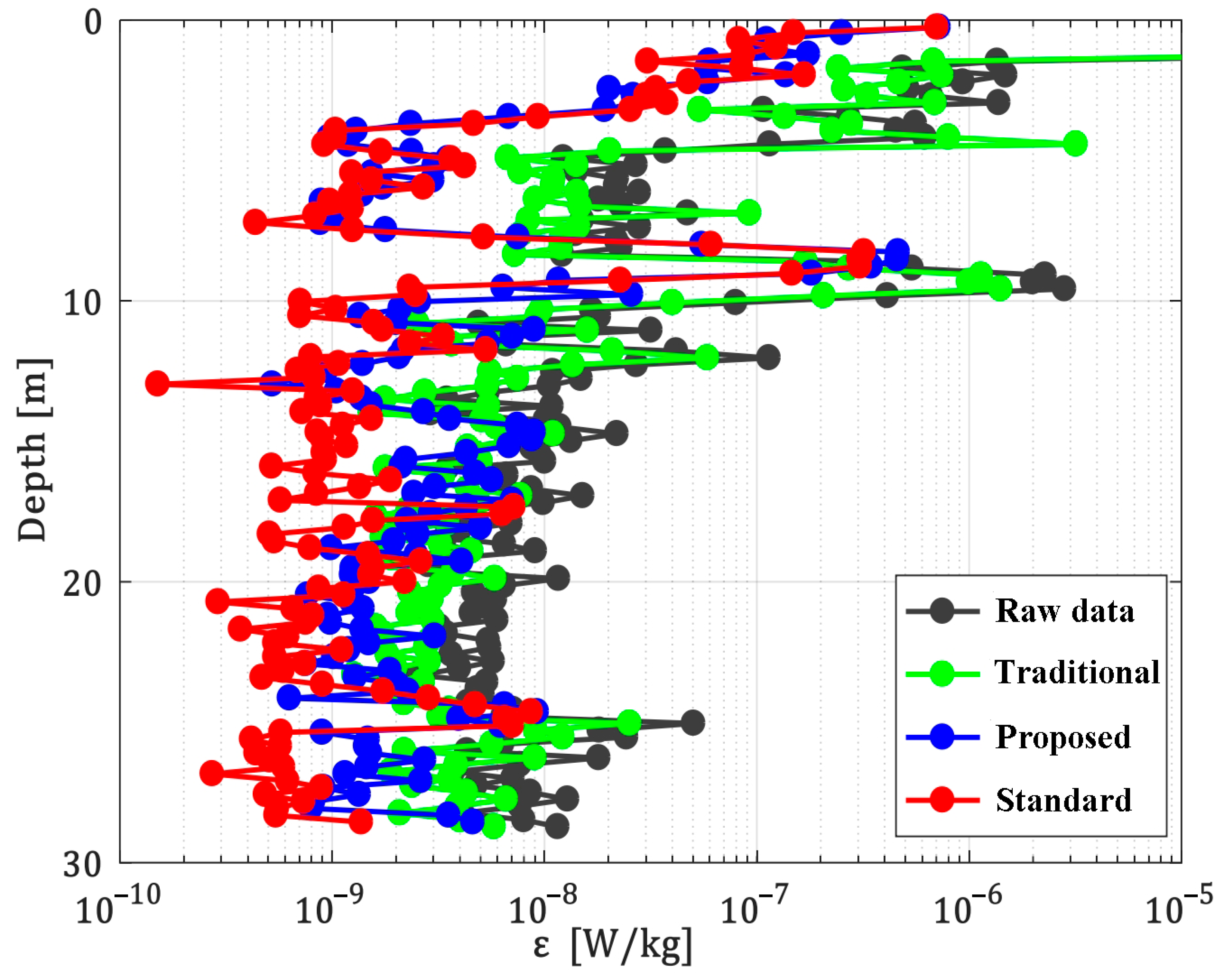
The variation in dissipation rate magnitude estimated from the original shear velocity spectra was approximately in the range from ${10}^{-6}$ WKg⁻¹ to ${10}^{-8}$ WKg⁻¹ (represented by black solid circles in Figure 11). Moreover, the dissipation rate variation obtained with the exclusive use of the CSCC algorithm (represented by green solid circles) displayed a less notable difference from the original profile. However, the corrected dissipation rates (represented by blue solid circles) obtained with the proposed MFNR method exhibited a significant decrease of over one order of magnitude. To verify the effectiveness of our method, the standard records were synchronously measured by the MicroRider instrument (manufactured by the Rockland Scientific International (RSI), Victoria, BC, Canada) and were also used to evaluate the dissipation rates (red solid circles). The dissipation rate variation calculated by the MFNR method aligned well with that obtained from standard records in the strong disturbance range (0–11 m) and was only slightly higher than the red profile in the weak disturbance range (11–30 m). This signifies that the proposed MFNR method is efficient in eliminating multi-frequency contamination induced by vibration and that it provides a purified shear signal for subsequent turbulence analysis.

4. Conclusions

In this work, an MFNR method based on secondary decomposition and the multi-mode coherence correction algorithm is proposed to suppress the noisy contamination contained in shear data, and the effectiveness of the proposed MFNR method is verified by the experimental measurements collected by using an AUV in Thousand Lake. The mechanical structure of AUVs causes multi-frequency noisy vibrations during turbulence measurements, obstructing the exploration of turbulence mechanisms. Conventional correction methods can only detect a part of prominent vibration features, and mixing modes still degrade data quality. Therefore, the thorough extraction of vibration information is critical for targeted noise suppression.

Turbulence measurements are complex nonlinear signals. Decomposing turbulence data into multi-frequency modes and conducting targeted correction is considered an effective way to suppress noisy contamination. Based on the results of frequency spectrum analysis, weak frequencies are amplified and isolated. Therefore, the complete central frequency series is obtained, providing identical frequency intervals to separate the raw measurements and the vibration signal, refining the vibration causality. Accompanied by acceleration modes in identical central frequency bands, the raw shear components allow for targeted correction. The vibration peaks in the wavenumber spectrum are obviously suppressed. Further, the cleaned shear spectrum, denoised by the MFNR method, agrees well with the standard Nasmyth spectrum, improving the quality of shear data. Practical applications show that dissipation rates evaluated from denoised shear spectra are reduced by almost an order of magnitude compared with the original profiles. The method proposed in this paper performs well in both strong and weak disturbance ranges.

As a consequence, the proposed noise correction method has the following dominant advantages: (1) Secondary decomposition extracts the residual information from the MMF and provides thorough multi-frequency information. (2) Secondary decomposition separates the shear and acceleration signals into several pairs of shear and acceleration modes with the same central frequencies based on the complete multi-frequency information. (3) Shear modes and acceleration modes with identical central frequencies provide the raw signal and its corresponding vibration-induced signal at the specific frequency. (4) The idea of multi-mode coherence correction is applied to each pair of shear and acceleration modes in identical frequency bands, which allows for targeted noisy vibration suppression. The result of the experimental analysis proves the superior performance of the proposed approach in suppressing the multi-frequency mechanical noise contained in the original shear signals. For future study, the proposed approach provides an optimal perspective on multi-mode noise correction for complicated turbulence data in the marine environment.