
Multi-View Synthesis of Sparse Projection of Absorption Spectra Based on Joint GRU and U-Net


State Key Laboratory of Dynamic Measurement Technology, North University of China, Taiyuan 030051, China
*
Author to whom correspondence should be addressed.
Appl. Sci. 2024, 14(9), 3726; https://0-doi-org.brum.beds.ac.uk/10.3390/app14093726
Submission received: 1 April 2024
/
Revised: 18 April 2024
/
Accepted: 25 April 2024
/
Published: 27 April 2024
(This article belongs to the Section Applied Physics General)
Abstract
:Tunable diode laser absorption spectroscopy (TDLAS) technology, combined with chromatographic imaging algorithms, is commonly used for two-dimensional temperature and concentration measurements in combustion fields. However, obtaining critical temperature information from limited detection data is a challenging task in practical engineering applications due to the difficulty of deploying sufficient detection equipment and the lack of sufficient data to invert temperature and other distributions in the combustion field. Therefore, we propose a sparse projection multi-view synthesis model based on U-Net that incorporates the sequence learning properties of gated recurrent unit (GRU) and the generalization ability of residual networks, called GMResUNet. The datasets used for training all contain projection data with different degrees of sparsity. This study shows that the synthesized full projection data had an average relative error of 0.35%, a PSNR of 40.726, and a SSIM of 0.997 at a projection angle of 4. At projection angles of 2, 8, and 16, the average relative errors of the synthesized full projection data were 0.96%, 0.19%, and 0.18%, respectively. The temperature field reconstruction was performed separately for sparse and synthetic projections, showing that the application of the model can significantly improve the reconstruction accuracy of the temperature field of high-energy combustion.
1. Introduction
In order to optimize combustion processes, improve combustion efficiency and reduce pollutant emissions, accurate and reliable measurements of temperature and gas component concentrations in combustion fields are of paramount importance. Taking the temperature measurement as an example, although the development of contact temperature measurement methods represented by thermocouples is relatively mature, most of them are single-point or wall temperature distribution measurements. Usually, multiple measurement points need to be deployed to reflect the temperature distribution within the combustion field, which cannot meet the demand for high-quality field distribution measurements, and the contact measurements will destroy the combustion flow field, affecting the measurement results [1,2]. In contrast, infrared thermography and radiation thermometry, as two types of non-contact measurement methods, do not interfere with the measurement area and more easily achieve the field distribution measurement [3,4], but these methods usually measure the temperature of the surface of the combustion field, and it is difficult to meet the needs of temperature measurement inside the combustion field.
Tunable diode laser absorption spectroscopy (TDLAS), known for its sensitivity, accuracy, reliability, and non-invasiveness, has become one of the most accurate in situ temperature and gas concentration measurement techniques for combustion diagnostics [5,6]. In particular, the method can optimize the combustion process, improve the efficiency of energy utilization, and reduce the generation of emissions by accurately monitoring the temperature, concentration, and other parameters of gasifiers, internal combustion engines, and aircraft engines, thereby achieving more environmentally friendly and efficient energy utilization. The application of this technology enables researchers to gain a deeper understanding of the details of the combustion process, providing strong support for the design, control, and optimization of combustion systems [7,8,9,10,11].
TDLAS measurement results represent the average values along the optical path and do not directly reflect the spatial distribution of information in the combustion field. To address this limitation, scholars have combined TDLAS technology with computed tomography (CT) imaging technology, proposing tunable diode laser absorption tomography (TDLAT). The two-dimensional distribution of parameters within the combustion field can be obtained by utilizing multiple intersecting laser beams. The bilinear ratio method is used, which involves selecting two laser beams of specific wavelengths and using the integral absorbance ratio obtained from the projection data to reconstruct the temperature and concentration values within each pixel grid. This method offers a dependable way to extract spatial data on temperature and concentration distributions in the combustion field [12].
In the field of combustion, many scholars have contributed to investigating and reconstructing temperature fields. Kristin et al., from the University of Virginia, measured the two-dimensional temperature distribution at the exit of a supersonic combustion wind tunnel using multi-angle and direct absorption spectral data from two water vapor lines combined with a classical filtered inverse projection algorithm [13,14]. Although the method produced satisfactory reconstruction results, it requires a large number of beams, which may be impractical for real-world applications. Xu, Liu et al. developed a pentagonal TDLAS detection system and used a modified Landweber algorithm to reconstruct two-dimensional temperature and water vapor concentration distribution in vortex combustion [15,16].
However, when dealing with a large amount of TDLAS projection data, challenges such as low reconstruction accuracy and slow processing speed arise. The rapid development of artificial intelligence has led to the widespread use of deep learning in combustion diagnostics. Compared to traditional reconstruction methods, deep learning offers excellent advantages in terms of reconstruction efficiency and accuracy [17,18,19]. To reconstruct nonlinear tomographic absorption spectra with limited data, Huang, Liu et al. used a convolutional neural network. The reconstruction process was accelerated, but satisfactory results required at least six projection views [20]. Chen, Hao et al. used a U-shaped residual network for super-resolution reconstruction of the temperature field [21]. Obtaining sufficient probe data can be challenging due to harsh test conditions in practical engineering applications. Although deep learning-based methods can produce laminar temperature field images with a limited number of angles, the quality of the reconstruction is relatively low. In addition, these methods do not fully exploit the sequential properties among the probe projection data to enhance the projection data and improve the temperature field reconstruction. It is a pressing issue in combustion diagnostics to ensure the quality of temperature field reconstruction with fewer projection views [22].
This paper proposes a neural network-based projection data enhancement algorithm named GMResUNet to address the problem of low accuracy in TDLAS detection reconstruction with limited detection projection angles. The network model utilizes the gate recurrent unit (GRU) and multilevel residual learning based on U-Net to achieve the multi-view synthesis of sparse projection data. The U-shaped deep learning network’s cross-connection structure ensures shallow correlation structuring while preserving the deep feature information of the integral absorbance data [23]. The multilevel residuals can learn the residual part more efficiently, reducing the number of parameters that need to be learned and improving the network’s efficiency and generalization ability [24]. The GRU can learn the sequence properties among the projection angles [25]. Compared to traditional interpolation methods and UNet, the GMResUNet proposed in this study exploits the sequence characteristics of the projection data from adjacent viewpoints to achieve multi-view synthesis of sparse projection data. The synthesized projection data significantly improve the reconstruction accuracy of the combustion temperature field, especially when there are only a small number of probe viewpoints.
2. Mathematical Background
2.1. Tunable Diode Laser Absorption Tomography
The TDLAS technique is a line-of-sight (LOS)-based path-integrated measurement technique characterized by fast response and high sensitivity. The technique is usually combined with computed tomography (CT) for the distribution measurements of gas temperatures, concentrations, and other parameters [26]. The basic theory of the TDLAS technique, the mathematical expression of Beer–Lambert’s law, can be described as:
In this equation, and represent the intensities of the outgoing and incoming laser beams, respectively. is the pressure in the region of interest, while is the concentration of absorbing molecules in the region. The linear strength of the absorbing molecules, denoted by , depends on the temperature . is the length of the optical path through which the beam is absorbed. is a linear function satisfying the normalization condition for . is the path-integrated absorbance.
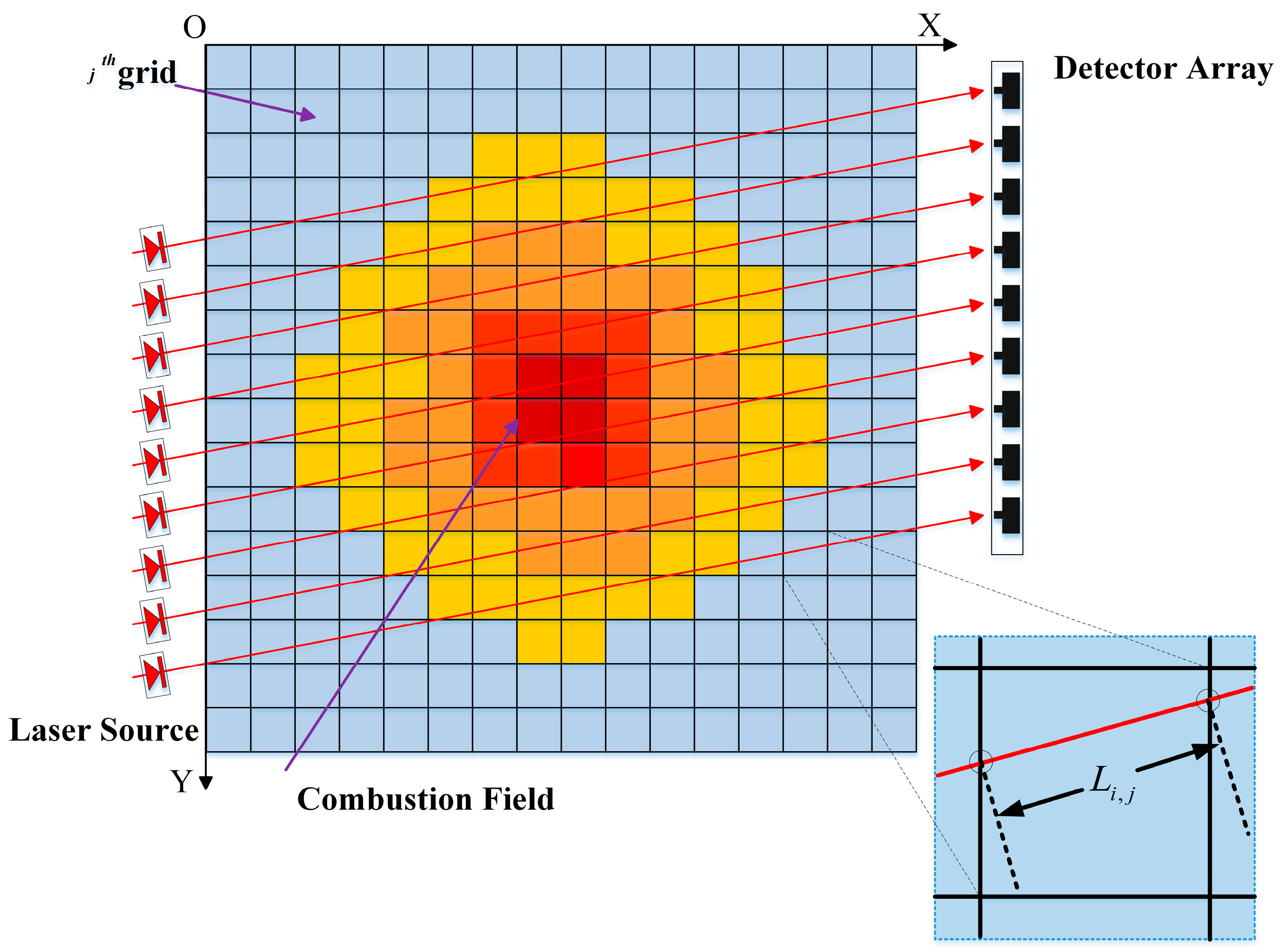
Figure 1 illustrates the importance of the individual physics of the TDLAT measurement system as the laser passes through the combustion field to be measured. For the non-uniform characteristics of the two-dimensional temperature distribution of the high-energy combustion field, the area to be measured can be divided into grids, and assuming that the distribution within each grid is uniform, i.e., the combustion field area is discretized, Equation (1) can be transformed into Equation (2):
The discretization formula of Equation (2) can be written in the form of a matrix:
where denotes the integral absorption value of the detection path of the th laser beam at frequency ; denotes the th grid number, and is the total number of grids in the discretized field; denotes the path length of the th laser beam through the th grid and the weight of the grid.
Under this discretized model, the problem of reconstructing the temperature distribution in the TDLAT system can be described as follows: solve the information asymmetry between the temperature distribution and the concentration distribution coupled according to the path integral absorption value and the lattice weights . In this paper, the two-dimensional reconstruction of the temperature field is realized by using the absorbance ratio of two absorption spectral lines according to the two-line ratio thermometry.
2.2. GRU Module for Absorbance Data
The gate recurrent unit (GRU) network is a kind of recurrent neural network (RNN). It deals with time series data. It can solve some complexity and computational overhead problems existing in the long short-term memory (LSTM) network [27,28]. It can also simplify the model structure to some extent and improve the training efficiency. For example, in the case of the stationary TDLAS temperature measurement system, the measurement of the combustion temperature field involves the measurement of the region of interest from multiple angles. The obtained projections represent the two-dimensional datasets obtained by the laminar scanning process. Each row of these data represents the projection of the laser absorption spectrum obtained by the detector at increasing angles. The features are sinusoidal throughout the image. Along a particular sinusoidal curve, the gray values of each detector element show a strong correlation. Therefore, we can treat each row of projected data as a sequence over the projected angle.
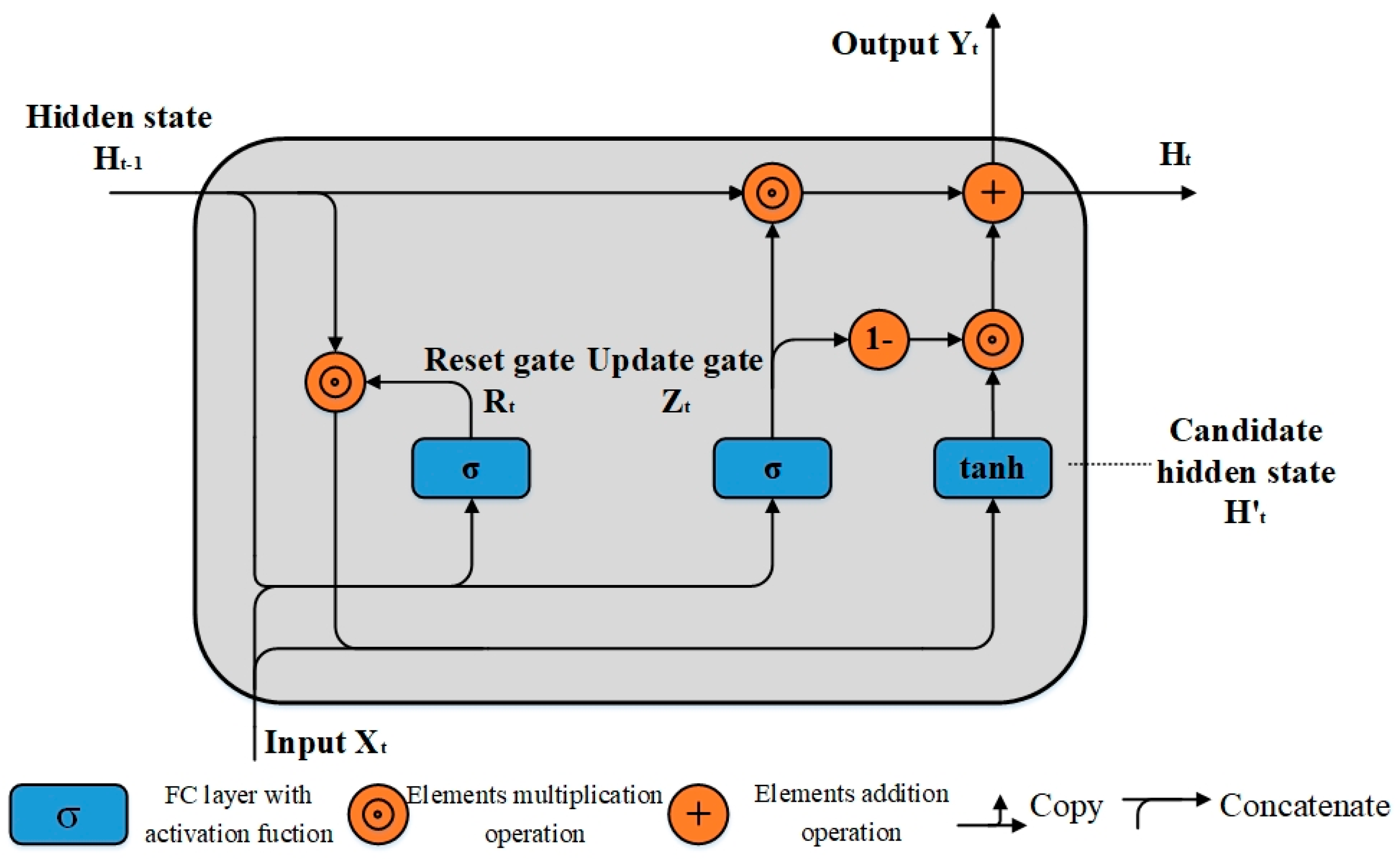
The GRU network shows excellent performance in processing sequential data, so the inherent sequential nature and sinusoidal correlation of projection data make it ideal for synthesizing sparse projection data. The structure of the GRU network cell is shown in Figure 2; it controls the flow of information through the network by introducing two gating mechanisms, namely the reset gate and the update gate, and updating then. These gating mechanisms help the GRU network to better capture the intrinsic relationships in the sequence of lines and rows of the projected data, with a smaller number of parameters compared to the LSTM network.
The flow of the projected data within the module is as follows:
At the th projection angle, Equation (5) defines the variable as the gate of the control reset of the projection data:
where is the absorbance data at the th projection angle; is the hidden state at the st projection angle, and this hidden state contains the relevant information about the previous projection angle; and denote the weight matrices corresponding to and , respectively, at the input of the reset gate; is the bias matrix of the reset gate; and is the activation function of the reset gate, which is essentially a nonlinear mapping sigmoid function that transforms the data into the range of 0–1 and acts as a gating signal. The variable is the gate for the control update of the absorbance data at the th projection angle, which is defined by Equation (6):
Similarly, is the activation function of the update gate; and are used as the inputs of the update gate; and denote the weight matrices corresponding to and at the input of the update gate, respectively; and is the bias matrix of the update gate. In Equation (7), the variable is the candidate hidden state at the projection angle t and is defined as follows:
where the data after the reset are obtained by resetting the Hadamard product of the gate and the hidden state of the projection angle. and denote the weights of the current input and the reset data, respectively, and is the bias for calculating the candidate hidden state at the projection angle t. The data are deflated to the range of −11 by the tanh activation function to obtain the candidate under the current projection angle t of the hidden state . It can be seen that mainly contains part of the information of the current input and the control by the reset gate as a way to memorize the information state of the current projection angle.
The variable is the hidden state under the current input , defined as in Equation (8):
where is the update gate, which controls how the hidden state of the previous moment is passed to the current moment and how the inputs of the current moment are integrated into the hidden state. Also, is the output of the GRU module in state t.
2.3. Residual Networks
Residual networks, with a very effective deep neural network architecture, are widely used, especially in image processing tasks. Traditional deep neural networks suffer from gradient vanishing and model degradation during training. The performance tends to deteriorate as the depth of the network increases. To address this problem, the concept of residual networks was proposed. The network is characterized by the inclusion of hopping connections that allow for information to bypass several layers and flow directly through the network. This structural innovation ensures smoother information propagation and avoids the problems of vanishing gradients and model degradation [29]. Residual networks can learn constant mappings more easily, avoiding information loss and loss of information. This allows the model to fit the training data better, improving the expressiveness and accuracy of the model. At the same time, residual networks also reduce the number of parameters and improve the computational efficiency of the network. Deeper training of the network is realized to extract more complex and abstract features. The structure of a single residual module is shown in Figure 3.
In this context, x represents the input, ReLU is the activation function, and and denote the mapping before and after the summation, respectively. The difference between residual network and traditional network structures is the inclusion of an extra hop connections that directly connect the input to the output layer, called shortcut connections, denoted as . Typically, represents the input x. If the mapping of inputs to the outputs of the channel is inconsistent, the number of channels in the residual connection is adjusted by convolving with a kernel of 1.
2.4. GMResUnet Structure
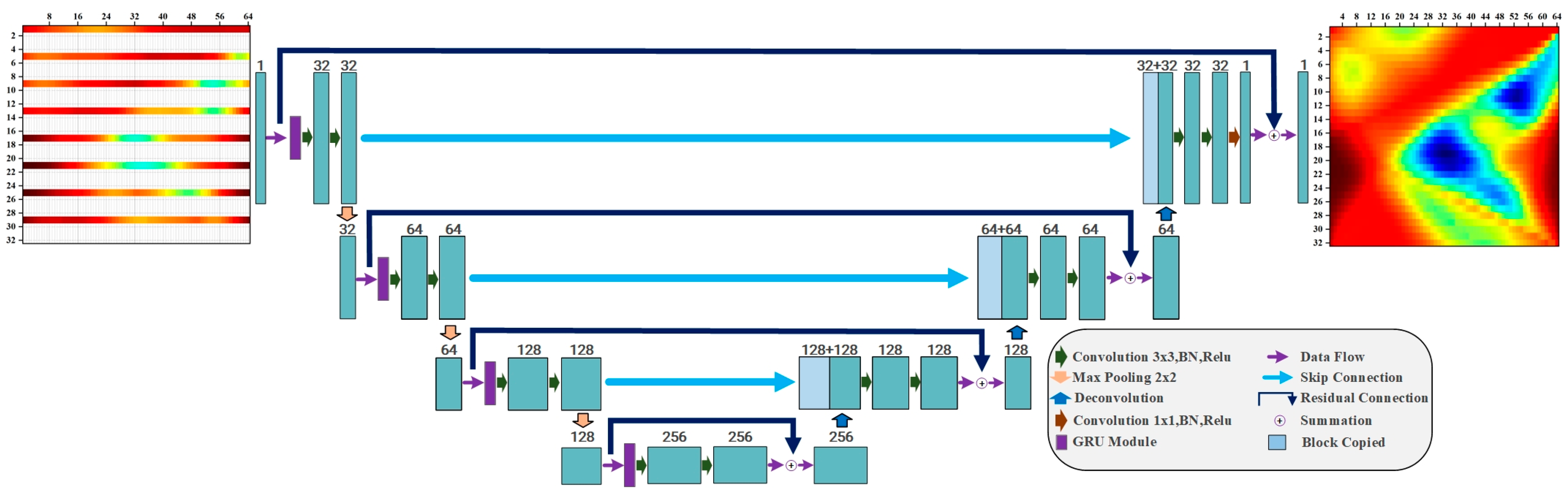
In this section, a sparse projection synthesis network is proposed, which incorporates the GRU network with multilevel residual connectivity on the basis of U-Net, and is named GMResUnet, as shown in Figure 4. The combination of the U-Net, the multilevel residual connectivity, and the GRU module with the learnable sequence feature has not been applied in the synthesis of laser absorption spectral projection data from sparse projections. Therefore, this study paid special attention to the sequence characteristics of the TDLAT projection data with respect to the projection angle, where the data from each detector are sinusoidally regular along the detection angle and where U-Net embodies a classical network architecture with encoding and decoding structures. Downsampling is accomplished through a series of successive convolutional and pooling layers, while upsampling involves successive convolutional and deconvolutional layers, with cascade connections between the corresponding layers.
The GMResUnet architecture consists of seven convolutional modules, four GRU modules, and multilevel residual connections.
During the encoding phase, the encoder’s coding module comprises a GRU module, two 3 × 3 convolutional layers, and a ReLU activation function. The GRU module extracts sequential features based on the projected view from the projected data, while the convolutional layers capture spatial features. The nonlinear activation function enhances the network’s expressive power. Increasing the number of channels enables the capture of rich semantic information. Additionally, a maximum pooling layer is utilized between each coding module to decrease the size of the feature mapping. This gradual downsampling process aids in broadening the sensory field and extracting global features.
During the decoding stage, the feature map’s spatial resolution is gradually restored through upsampling while simultaneously reducing the number of channels. The decoder’s decoding module comprises an inverse convolutional layer and an activation function that gradually recovers the feature map’s spatial dimensions. The inverse convolutional layer’s gradual upsampling operation recovers detailed image information and enables fine modeling of the local features. Additionally, each decoding module in the decoder is fused twice with the corresponding feature map of the encoder to introduce low-level fine-grained information. Two methods are used to connect the feature maps of the encoder and decoder levels in image restoration. The first method involves splicing the feature maps element-by-element, while the second method involves the summation of the initial feature maps with the feature maps in the decoder via residual connection. The use of jump connections helps to convey low-level details and boundary information, resulting in better restoration of the original image. Additionally, the introduced multilevel residual connections provide noise immunity.
By adding the inputs and outputs directly and using jump connections to introduce low-level features into the high-level computation, the network can focus more on the difference between the inputs and outputs. This approach is relatively insensitive to noise because it fits the difference between the inputs and outputs by learning the residual function. Residual learning can improve the network’s robustness to noise, accelerate its convergence, and better synthesize sparse projection data. The network uses zero-padding to maintain input and output image size during training. The last convolutional module in the decoding stage has a kernel size of 1, ensuring that each pixel corresponds to a category label.
In the GMResUNet framework, the encoder’s convolution operation is preceded by the GRU module. The data from the projected viewpoints are treated as time-series data, with each row representing a sequence. This sequence is then recursively processed in behavioral units by the GRU module.
Figure 5 shows the data flow of this module assuming projection angles. represents the projection data at the th projection angle, which serve as the input to the GRU unit. is the output corresponding to the last hidden layer. The n outputs are spliced as input features to the convolutional layer. The convolutional layer can include the sequence features of the projection data at adjacent viewpoints, achieving deep fusion of spatial and sequence information [30].
3. Settings for Simulative Studies
This section presents a simulation study that validates the feasibility of the GMResUNet for synthesizing multi-view absorbance data. This study included dataset preparation, network training, and quality assessment.
3.1. Dataset Preparation
Gaussian flames were utilized to simulate real flames, and a stochastic mixed Gaussian flame model was constructed to generate Gaussian flames with varying numbers of peaks and peaks with stochasticity [31,32]. This approach enables the simulation of complex temperature distributions in actual combustion fields. A total of 20,000 temperature distribution samples were manually created. These simulated samples described a typical combustion temperature range from 800 K to 2600 K and included one to three randomly distributed Gaussian peaks. A visual representation of these temperature distributions is depicted in Figure 6.
Numerical simulations were conducted to model the process of temperature field probing using the TDLAS technique. The network training used 16,000 samples, while 2000 samples were used for network validation, and another 2000 samples for network testing. Each sample consisted of five types of projection data captured using a 64-way detector in the formats of 2 × 64, 4 × 64, 8 × 64, 16 × 64, and 32 × 64. The projection data with the size specification of 32 × 64 were designated as the labeling data, while the other sparse projection data were used as the network input for the synthesis of the multi-angle projection data. Figure 7 shows the label projection data corresponding to the three typical temperature fields simulated in Figure 6.
Taking the projection data corresponding to the complex multi-peak temperature field as an example, each projection data sample contained projections with different sparsity levels, as shown in Figure 8. The white area is the projection angle to be synthesized, and the data preprocessing fills it with zeros, which ensures the same resolution of the network inputs and outputs.
3.2. Network Training and Implementation
The GMResUNet proposed in this study was trained using the PyTorch framework with an L2 loss function, defined as follows [33]:
where N is the total number of samples in each batch of projected data, and K is the total number of pixels in each distribution. The variables and refer to the ground truth and predicted values of the k-th pixel, respectively. The training process consisted of repeating the batch until the loss function converged.
The optimizer used was the adaptive moment estimation (Adam) [34] optimization method, which combines the concepts of the RMSprop algorithm and the momentum-based approach to not only implement momentum-driven parameter updates but also to adaptively adjust the learning rate to improve the gradient descent. Compared to other adaptive learning rate algorithms, Adam converges faster and learns better. The network was trained on an NVIDIA GeForce RTX 3090 GPU with a learning rate of 2.6 × 10⁻⁴ and a training time of nearly 10 h.
The validation set was used during training to assess the model convergence to avoid network overfitting. In the validation set, the network parameters were not updated. In Figure 9, two plots show the evolution of the loss function for the training and validation sets under four sparse projection data. It can be observed that the model converged quickly in the first 300 periods on the training set and gradually stabilized after 300 periods; the validation set shows a similar pattern, so the network was not overfitted. In particular, the model converged slowly when N = 2 and quickly for N > 2 (N = 4, 8, 16). The results show that the model converged faster as the richness of the projected data increased; the difference in the convergence of the loss function was smaller for projection angles N above 4.
3.3. Indexes of the Quality Assessment
To evaluate the performance of the GMResUnet, we defined three metrics to evaluate the effect of sparse projection data synthesized into multi-angle projection data, i.e., the difference between the predicted values and the real labeled dataset, as the peak signal-to-noise ratio (PSNR), structural similarity (SSIM), and the projection data synthesis error [35]. These performance metrics are defined as follows:
The peak signal-to-noise ratio (PSNR) is the ratio of the maximum power of the signal to the noise power of the signal in decibels (dB). It is defined based on the mean square error (MSE) for the given original image I of size m × n and a noisy image K to which noise has been added. Its MSE and PSNR are defined as:
where m and n are the length and width dimensions of the image respectively; MSE is the mean square error; I is the true value; K is the predicted value; and is the maximum possible pixel value in the image.
The structural similarity (SSIM) is a measure of the similarity of two images. The closer the SSIM value is to 1 means that the two images are more similar. The specific mathematical representation is:
where x and y are the original and reconstructed images, respectively; and are the mean values corresponding to the images x and y, respectively; and are the variance of the images, respectively; is the covariance of x and y; and and are the constants used to maintain stability, where L is the range of pixels of the images x and y, usually taken as , .
The relative error represents the error between the generated values of the projection data and the labeled data:
where Δ is the absolute error; L is the true value; and are the true and generated values of the th pixel of the projection data matrix, respectively, and N is the total number of pixels of the absorbance data.
4. Results and Discussion
4.1. Image Reconstruction Results
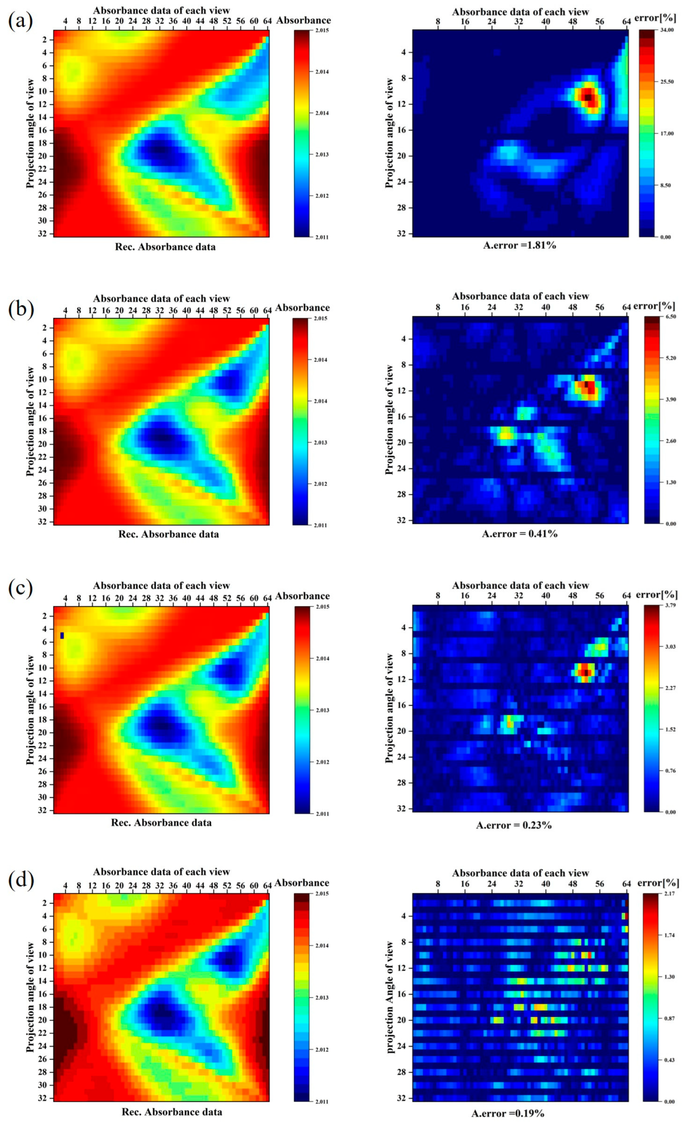
The projection data with different specifications in the test set were fed into the trained GMResUNet model to generate the multi-angle projection data matrix (N = 32). As shown in Figure 10, Figure 11 and Figure 12, the synthesized typical single-peak, double-peak, and multi-peak temperature field multi-angle projection data and error map distributions under the conditions of N = 2, 4, 8, and 16 are shown, respectively, with the generated multi-angle projection data on the left and the corresponding relative error distributions on the right. Table 1 shows the average relative errors of the four sparse projection data for the three temperature field modes.
It can be seen that as the complexity of the temperature field increased, the normalized error of the synthetic multi-angle projection data of this network remained below 0.5% under the number of projections of N = 4 and above. Under the extremely sparse projection probing of N = 2, the normalized error of its synthetic multi-angle data was less than 0.8% for the single-peak and double-peak temperature fields, and greater than 1% for the multi-peak temperature field due to its complexity.
In order to evaluate the quality of the complete projection data generated by the GMResUnet, the temperature distributions of the synthesized projection data were reconstructed using typical CNN [20] algorithms available in the literature, as well as a reconstruction network based on the U-Net framework, as shown in Figure 13. The PSNR, SSIM, and relative error were also used as specific metrics to evaluate their quality for temperature field reconstruction.
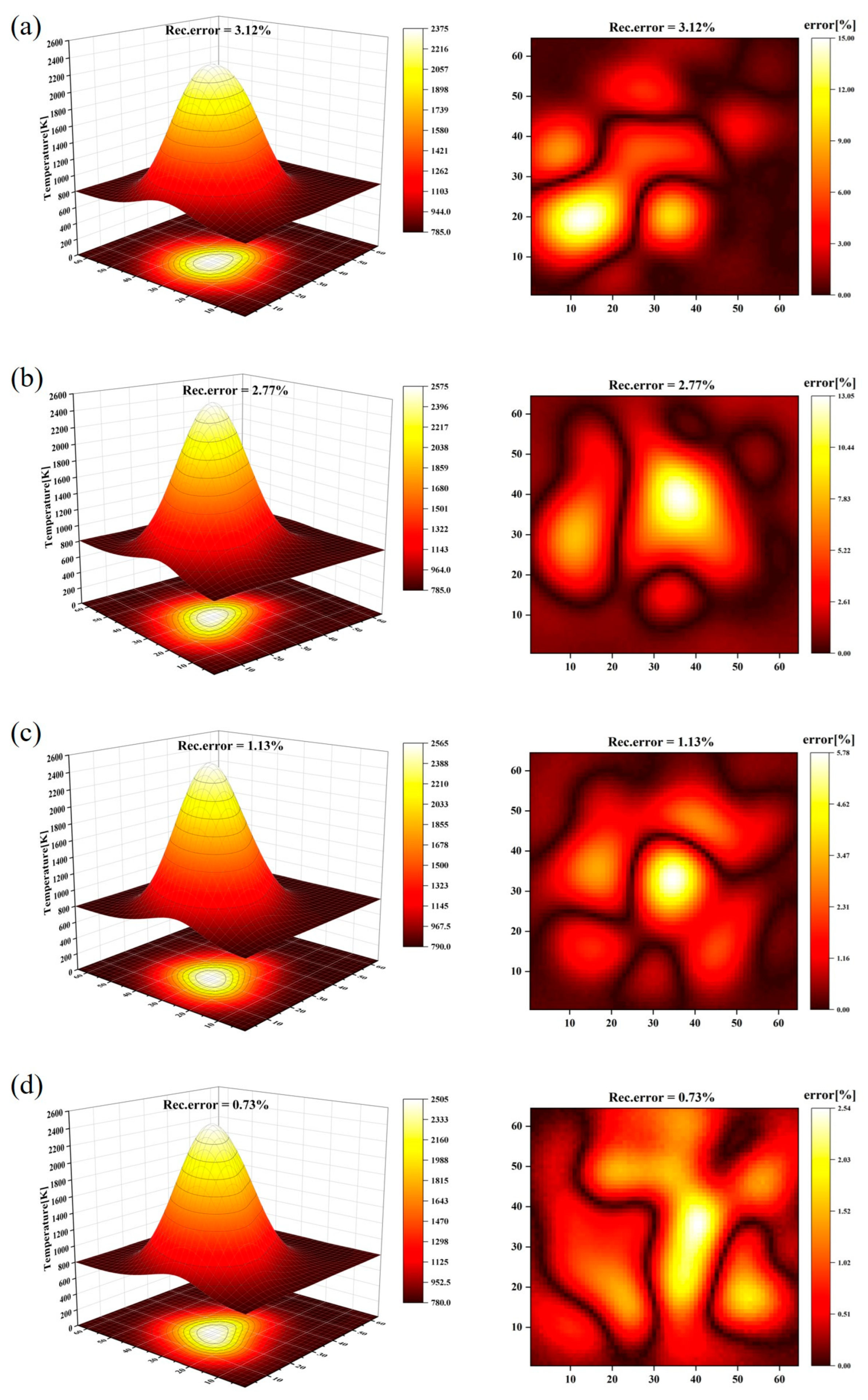
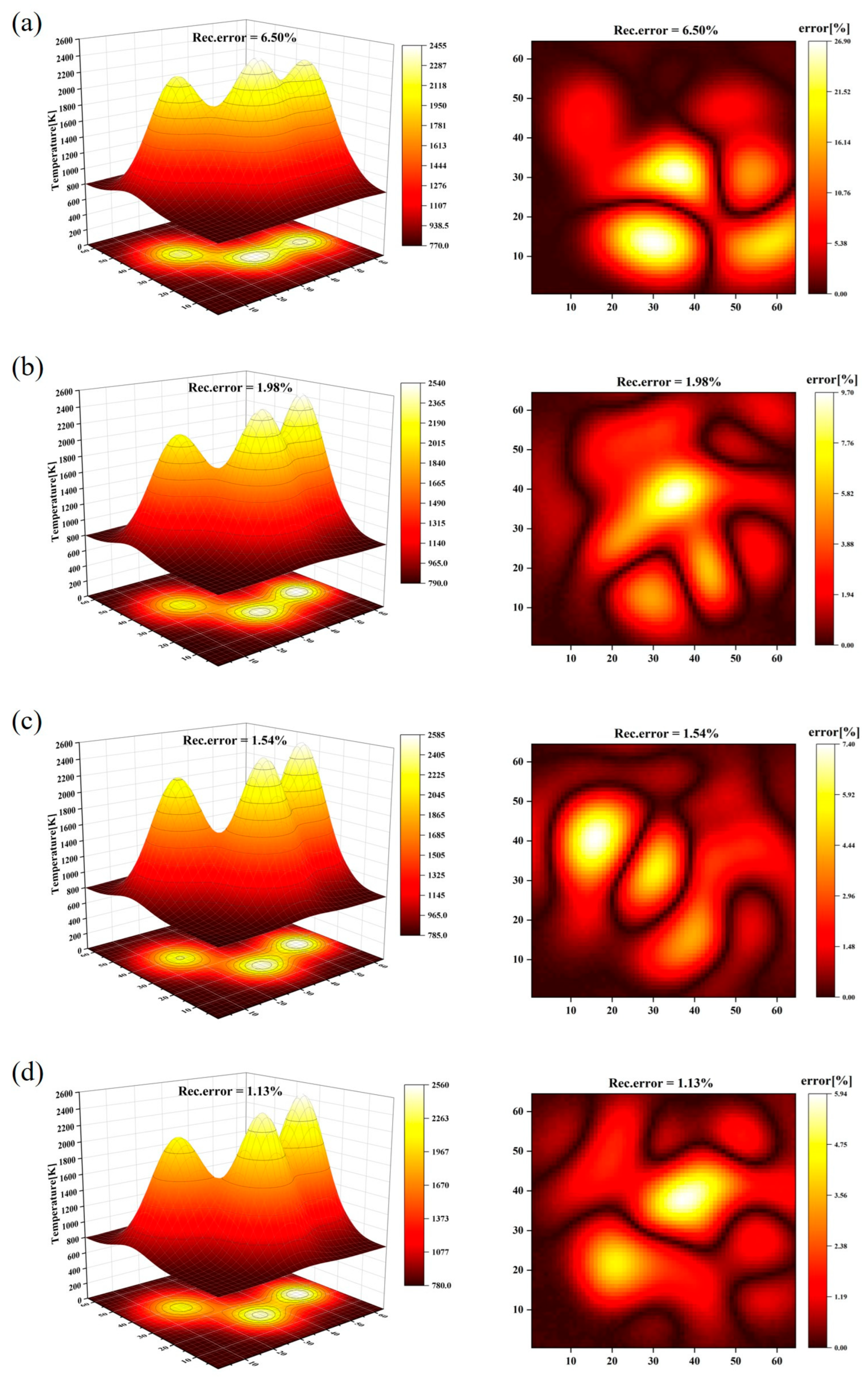
The U-Net was used to evaluate the effect of the synthesized temperature field reconstruction, as shown in Figure 14, Figure 15 and Figure 16, which represent typical single-peak, double-peak, and multi-peak temperature fields reconstructed under the N = 2, 4, 8, and 16 conditions, as well as the relative error plots. The network input projection data correspond to the multi-angle projection data synthesized in Figure 10, Figure 11 and Figure 12. Table 2 shows the reconstruction errors of the three temperature fields.
The results show that the reconstruction error of the temperature field was less than 2% for N = 4 and above, and the reconstruction error of the single-peak and double-peak temperature fields was less than 3.5% for the extremely sparse projection probe with N = 2. This means that this sparse projection synthesis method can be widely applied to synthesize probe data for various distributions. The basic trend of the reconstruction error was to increase with the increase in the complexity of the temperature field and to decrease with the increase in the number of projections, N. However, the reconstruction error of the multi-peak complex temperature field under the condition of N = 2 was still less than 7%, although the synthesis of its corresponding projection data was less effective. On the other hand, the error of the highest temperature peaks with drastic changes was slightly larger than that of the places with gentle changes, which may be determined by the theory of molecular absorption spectroscopy, where the absorption sensitivity of molecules decreases with an increasing temperature. Especially in the case of the extremely high temperature of 2600 K in the present simulation, the neural network may not be able to decouple the feature mapping of higher-temperature values very well [36,37].
4.2. Evaluation of Indicators
In order to quantitatively analyze the effects of multi-angle projection data synthesis, the PSNR, SSIM, and error of the -angle data synthesis metrics for different sparse projections were calculated on the test set with 2000 samples. As shown in Table 3, we applied three methods to calculate the PSNR, SSIM, and error of different sparse projections for N = 2, 4, 8, and 16 data, respectively, and the results are the average values of 2000 data on the test set. The three synthesized methods are the interpolation method, the UNet, and the GMResUNet.
In Table 3, it can be seen that the results of the interpolation method were the worst in all three metrics, while the UNet performed better than the interpolation method, and GMResUNet performed the best among the three. Regarding errors, the GMResUNet had the lowest results, the interpolation method had significantly higher results, and the UNet performed well. These results show that the GMResUNet can maintain high-quality synthesis of sparse to multi-angle projections and achieve further improvement of the projection data.
In order to evaluate the quality of temperature field reconstruction of the synthesized multi projection data, the synthesized multi-angle projection data were also subjected to temperature field reconstruction on the test set with a sample of 2000. As shown in Table 4, we applied two methods to calculate the evaluation metrics of the temperature field under N = 2, 4, 8, and 16, and the results are the average values of the test set. Two of the synthesized methods were based on traditional CNN and U-Net and were specially trained for temperature field reconstruction in this paper. It can be observed that as the sparse angle N increased, the results of both the CNN and the U-Net reconstruction became significantly better, with the PSNR, SSIM, gradually increasing, and the error gradually decreasing. This proves that our proposed GMResUNet can realize the improvement of sparse projection, and thus, maintain the high quality of temperature field reconstruction in the sparse TDLAS technique for tomographic imaging tasks.
The quality analysis of temperature field reconstruction with limited projection data and synthetic projection data using the same reconstruction U-Net is shown in Table 5. It can be seen that the algorithm proposed in this section, which synthesizes a small amount of projection data into multi-angle data, enhanced the input data of the network well, and the quality of the reconstructed temperature field was obviously improved.
4.3. Noise Resistance Analysis of the Algorithm
To evaluate the noise immunity of the GMResUNet, Gaussian noise ranging from 0% to 12% was added to the original sparse projection data. As shown in Figure 17a, the average relative error after the synthesis of various types of sparse projections increases with the increase of noise intensity. Overall, the projected views with N = 16 are highly resistant to interference in the synthesis, and the average relative error of the synthesized multi projection data is less than 1%. When the noise level reaches 12%, the average relative error of projection number synthesis for N = 4 and above is less than 1.5%; while when N = 2, the average error of multi projection data synthesis is relatively large and has the worst anti-interference ability. In addition, the effect of noise on the quality of temperature field reconstruction was also investigated. As shown in Figure 17b, a similar trend was found in the reconstructed temperature field. For N = 4 and above, the reconstruction error remained below 8%. As the noise level increased, the temperature field reconstruction using the full projection data synthesized from N = 2 encountered significant errors and larger fluctuations.
5. Conclusions
In this paper, a neural network-based projection data enhancement algorithm is proposed to address the problem of low accuracy in TDLAS detection reconstruction using limited detection projection angles. The network model incorporates GRU and multi-level residual learning based on U-Net to realize the multi-view synthesis of sparse projection data. The cross-connection structure of the U-type deep learning network ensures a shallow correlation structurality with the premise of guaranteeing deeper feature information of the projection data. The multilevel residual learning of the higher-level feature representation, which improves the efficiency and generalization ability of the network, makes it easier to optimize and converge the network. The GRU is capable of learning the sequence properties among projection angles.
The feasibility of the network model was evaluated using numerical simulation methods, and an experimental study was conducted to synthesize 32 multi-angle projection data from a finite number of projection angles. Realizing the -fold enhancement of the projection data, the experimental results show that the GMResUNet algorithm has an excellent projection data synthesis ability. Its 8-fold synthesis ability was especially effective (sparse projection N = 4); the PSNR was 40.726, the SSIM was 0.997, and the average relative error was 0.35%. At the same time, the sparse projection and synthetic projection are used separately for temperature field reconstruction, and the results show that the synthetic ability of the algorithm can significantly improve the reconstruction accuracy of the high-energy combustion temperature field, especially in cases of a small number of detection perspectives. The algorithm can not only realize high-quality temperature distribution reconstruction with a small number of projections but also has a potential market economic value for simplifying the hardware composition of detection systems in the future.
Author Contributions
Conceptualization, Y.S.; methodology, Y.S.; software, Y.S.; validation, Y.S.; formal analysis, Y.S. and X.H. (Xiaojian Hao); investigation, Y.S. and X.H. (Xiaodong Huang); writing—original draft preparation, Y.S. and P.P.; writing—review and editing, Y.S. and P.P.; visualization, Y.S.; funding acquisition, X.H. (Xiaojian Hao), S.L. and T.W. All authors have read and agreed to the published version of the manuscript.
Funding
This work was supported in part by the National Natural Science Foundation of China (NSFC) under grant 52075504; the State Key Laboratory of Quantum Optics and Quantum Optics Devices (No. KF202301); the Shanxi Province Graduate Practice Innovation Project (2023SJ209); the Shanxi Province Graduate Practice Innovation Project (2023KY608); the Shanxi Provincial Key Research and Development Project (202302150101016); and Shanxi 1331 Project Key Subject Construction.
Institutional Review Board Statement
Not applicable.
Informed Consent Statement
Not applicable.
Data Availability Statement
The data presented in this study are available within the article.
Conflicts of Interest
The authors declare no conflicts of interest.
References
- Kim, D.; Kubota, Y.; Izato, Y.; Miyake, A. Temperature variation measurements of an ignited energetic ionic liquid. Sci. Technol. Energ. Mater. 2023, 84, 14–16. [Google Scholar]
- Manjhi, S.K.; Kumar, R. Surface heat flux measurements for short time-period on combustion chamber with different types of coaxial thermocouples. Exp. Heat Transf. 2020, 33, 282–303. [Google Scholar] [CrossRef]
- Stoukatch, S.; Dupont, F.; Laurent, P.; Redouté, J.-M. Package Design Thermal Optimization for Metal-Oxide Gas Sensors by Finite Element Modeling and Infra-Red Imaging Characterization. Materials 2023, 16, 6202. [Google Scholar] [CrossRef] [PubMed]
- Zhao, Y.; Lv, J.; Zheng, K.; Tao, J.; Qin, Y.; Wang, W.; Wang, C.; Liang, J. Multispectral radiometric temperature measurement algorithm for turbine blades based on moving narrow-band spectral windows. Opt. Express 2021, 29, 4405–4421. [Google Scholar] [CrossRef] [PubMed]
- Huang, A.; Cao, Z.; Zhao, W.; Zhang, H.; Xu, L. Frequency Division Multiplexing and Main Peak Scanning WMS Method for TDLAS Tomography in Flame Monitoring. IEEE Trans. Instrum. Meas. 2020, 69, 9087–9096. [Google Scholar] [CrossRef]
- Lackner, M. Tunable diode laser absorption spectroscopy (TDLAS) in the process industries—A review. Rev. Chem. Eng. 2007, 23, 65–147. [Google Scholar] [CrossRef]
- Bolshov, M.A.; Kuritsyn, Y.A.; Romanovskii, Y.V. Tunable diode laser spectroscopy as a technique for combustion diagnostics. Spectrochim. Acta Part B At. Spectrosc. 2015, 106, 45–66. [Google Scholar] [CrossRef]
- Gao, Y.G.; Liu, Y.; Dong, Z.C.; Ma, D.; Yang, B.; Qiu, C.C. Preliminary experimental study on combustion characteristics in a solid rocket motor nozzle based on the TDLAS system. Energy 2023, 268, 126741. [Google Scholar] [CrossRef]
- Song, A.C.; Qin, Z.; Li, J.W.; Li, M.; Huang, K.; Yang, Y.J.; Wang, N.F. Real-Time Plume Velocity Measurement of Solid Propellant Rocket Motors Using TDLAS Technique. Propellants Explos. Pyrotech. 2021, 46, 636–653. [Google Scholar] [CrossRef]
- Wang, J.; Hao, X.J.; Pan, B.W.; Huang, X.D.; Sun, H.L.; Pei, P. Spectroscopic measurement of the two-dimensional flame temperature based on a perovskite single photodetector. Opt. Express 2023, 31, 8098–8109. [Google Scholar] [CrossRef]
- Liu, X.; Hao, X.; Xue, B.; Tai, B.; Zhou, H. Two-dimensional flame temperature and emissivity distribution measurement based on element doping and energy spectrum analysis. IEEE Access 2020, 8, 200863–200874. [Google Scholar] [CrossRef]
- Nadir, Z. A Model Based Iterative Reconstruction Approach to Tunable Diode Laser Absorption Tomography. Ph.D. Thesis, Purdue University, West Lafayette, IN, USA, 2018. [Google Scholar]
- Bryner, E.; Sharma, M.; Diskin, G.; Mcdaniel, J.; Goyne, C.; Snyder, M.; Martin, E.; Krauss, R. Tunable Diode Laser Absorption Technique Development for Determination of Spatially Resolved Water Concentration and Temperature. In Proceedings of the 48th AIAA Aerospace Sciences Meeting Including the New Horizons Forum & Aerospace Exposition, Orlando, FL, USA, 4–7 January 2010. [Google Scholar]
- Martin, E.F.; Goyne, C.P.; Diskin, G.S. Analysis of a Tomography Technique for a Scramjet Wind Tunnel. Int. J. Hypersonics 2010, 1, 173–179. [Google Scholar] [CrossRef]
- Huang, A.; Cao, Z.; Zhao, W.; Zhang, H.; Xu, L. Fast Wavelength Modulated TDLAS Imaging System for Flame monitoring. In Proceedings of the 2019 IEEE International Instrumentation and Measurement Technology Conference (I2MTC), Auckland, New Zealand, 20–23 May 2019. [Google Scholar]
- Liu, C.; Cao, Z.; Lin, Y.Z.; Xu, L.J.; McCann, H. Online Cross-Sectional Monitoring of a Swirling Flame Using TDLAS Tomography. IEEE Trans. Instrum. Meas. 2018, 67, 1338–1348. [Google Scholar] [CrossRef]
- Xue, B.; Hao, X.; Liu, X.; Han, Z.; Zhou, H. Simulation of an NSGA-III Based Fireball Inner-Temperature-Field Reconstructive Method. IEEE Access 2020, 8, 43908–43919. [Google Scholar]
- Deng, A.; Huang, J.; Liu, H.; Cai, W. Deep learning algorithms for temperature field reconstruction of nonlinear tomographic absorption spectroscopy. Meas. Sens. 2020, 10, 100024. [Google Scholar] [CrossRef]
- Li, H.; Ren, T.; Liu, X.; Zhao, C. U-Net applied to retrieve two-dimensional temperature and CO2 concentration fields of laminar diffusion flames. Fuel 2022, 324, 124447. [Google Scholar] [CrossRef]
- Huang, J.; Liu, H.; Dai, J.; Cai, W. Reconstruction for limited-data nonlinear tomographic absorption spectroscopy via deep learning. J. Quant. Spectrosc. Radiat. Transf. 2018, 218, 187–193. [Google Scholar] [CrossRef]
- Chen, S.; Hao, X.; Pan, B.; Huang, X. Super-resolution residual U-Net model for the reconstruction of limited-data tunable diode laser absorption tomography. ACS Omega 2022, 7, 18722–18731. [Google Scholar] [CrossRef] [PubMed]
- Liu, C.; Tsekenis, S.-A.; Polydorides, N.; McCann, H. Toward customized spatial resolution in TDLAS tomography. IEEE Sens. J. 2018, 19, 1748–1755. [Google Scholar] [CrossRef]
- Han, Y.; Ye, J.C. Framing U-Net via Deep Convolutional Framelets: Application to Sparse-View CT. IEEE Trans. Med. Imaging 2018, 37, 1418–1429. [Google Scholar] [CrossRef] [PubMed]
- Wu, Z.; Zhao, L.; Zhang, H. MR-UNet commodity semantic segmentation based on transfer learning. IEEE Access 2021, 9, 159447–159456. [Google Scholar] [CrossRef]
- Chung, J.; Gulcehre, C.; Cho, K.; Bengio, Y. Empirical Evaluation of Gated Recurrent Neural Networks on Sequence Modeling. arXiv 2014, arXiv:1412.3555. [Google Scholar]
- Sun, P.; Zhang, Z.; Li, Z.; Guo, Q.; Dong, F. A Study of Two Dimensional Tomography Reconstruction of Temperature and Gas Concentration in a Combustion Field Using TDLAS. Appl. Sci. 2017, 7, 990. [Google Scholar] [CrossRef]
- Nosouhian, S.; Nosouhian, F.; Khoshouei, A.K. A review of recurrent neural network architecture for sequence learning: Comparison between LSTM and GRU. Preprints 2021, 2021070252. [Google Scholar] [CrossRef]
- Yamak, P.T.; Yujian, L.; Gadosey, P.K. A comparison between ARIMA, LSTM, and GRU for time series forecasting. In Proceedings of the 2019 2nd International Conference on Algorithms, Computing and Artificial Intelligence, Sanya, China, 20–22 December 2019; pp. 49–55. [Google Scholar]
- Targ, S.; Almeida, D.; Lyman, K. Resnet in Resnet: Generalizing residual architectures. arXiv 2016, arXiv:1603.08029. [Google Scholar]
- Li, S.; Ye, W.; Li, F. LU-Net: Combining LSTM and U-Net for sinogram synthesis in sparse-view SPECT reconstruction. Math. Biosci. Eng. 2022, 19, 4320–4340. [Google Scholar] [CrossRef] [PubMed]
- Si, J.J.; Fu, G.C.; Cheng, Y.B.; Zhang, R.; Enemali, G.; Liu, C. A Quality-Hierarchical Temperature Imaging Network for TDLAS Tomography. IEEE Trans. Instrum. Meas. 2022, 71, 4500710. [Google Scholar] [CrossRef]
- Zhao, R.; Zhou, B.; Zhang, J.; Cheng, R.; Liu, Q.; Dai, M.; Wang, B.; Wang, Y. Rapid online tomograph in non-uniform complex combustion fields based on laser absorption spectroscopy. Exp. Therm. Fluid Sci. 2023, 147, 110930. [Google Scholar] [CrossRef]
- Janocha, K.; Czarnecki, W.M. On loss functions for deep neural networks in classification. arXiv 2017, arXiv:1702.05659. [Google Scholar] [CrossRef]
- Mehta, S.; Paunwala, C.; Vaidya, B. CNN Based Traffic Sign Classification Using Adam Optimizer. In Proceedings of the 2019 international conference on intelligent computing and control systems (ICCS), Madurai, India, 15–17 May 2019; pp. 1293–1298. [Google Scholar]
- Sara, U.; Akter, M.; Uddin, M.S. Image quality assessment through FSIM, SSIM, MSE and PSNR—A comparative study. J. Comput. Commun. 2019, 7, 8–18. [Google Scholar] [CrossRef]
- Li, R.J.; Li, F.; Lin, X.; Yu, X.L. Error Analysis of Integrated Absorbance for TDLAS in a Nonuniform Flow Field. Appl. Sci. 2021, 11, 10936. [Google Scholar] [CrossRef]
- Lin, S.; Chang, J.; Sun, J.C.; Xu, P. Improvement of the Detection Sensitivity for Tunable Diode Laser Absorption Spectroscopy: A Review. Front. Phys. 2022, 10, 853966. [Google Scholar] [CrossRef]
Figure 1.
Schematic of the discretization method for the temperature field under measurement.

Figure 2.
Structure of GRU network cells.

Figure 3.
Structure diagram of the residual module.

Figure 4.
GMResUnet framework.

Figure 5.
Data flow diagram of the GRU module.

Figure 6.
Simulation of the temperature field distribution at a 64 × 64 resolution. (a) Single peak; (b) double peak; (c) multiple peaks.
Figure 6.
Simulation of the temperature field distribution at a 64 × 64 resolution. (a) Single peak; (b) double peak; (c) multiple peaks.

Figure 7.
Multi-angle projection data of three typical temperature fields (N = 32). (a) Single peak; (b) double peak; (c) multiple peaks.
Figure 7.
Multi-angle projection data of three typical temperature fields (N = 32). (a) Single peak; (b) double peak; (c) multiple peaks.

Figure 8.
Projection data for different sparsity levels. (a) N = 2; (b) N = 4; (c) N = 8; (d) N = 16.
Figure 8.
Projection data for different sparsity levels. (a) N = 2; (b) N = 4; (c) N = 8; (d) N = 16.

Figure 9.
Evolution of the loss function with training cycles for 4 sparse projection data. (a) Training set; (b) validation set.
Figure 9.
Evolution of the loss function with training cycles for 4 sparse projection data. (a) Training set; (b) validation set.

Figure 10.
Synthesis results and error distributions of four sparse projections of the single-peak temperature field. (a) N = 2; (b) N = 4; (c) N = 8; (d) N = 16.
Figure 10.
Synthesis results and error distributions of four sparse projections of the single-peak temperature field. (a) N = 2; (b) N = 4; (c) N = 8; (d) N = 16.

Figure 11.
Synthesis results and error distributions of four sparse projections of the bimodal temperature field. (a) N = 2; (b) N = 4; (c) N = 8; (d) N = 16.
Figure 11.
Synthesis results and error distributions of four sparse projections of the bimodal temperature field. (a) N = 2; (b) N = 4; (c) N = 8; (d) N = 16.

Figure 12.
Synthesis results and error distributions of four sparse projections of the multi-peak temperature field. (a) N = 2; (b) N = 4; (c) N = 8; (d) N = 16.
Figure 12.
Synthesis results and error distributions of four sparse projections of the multi-peak temperature field. (a) N = 2; (b) N = 4; (c) N = 8; (d) N = 16.

Figure 13.
U-Net temperature field reconstruction model for test projection data.

Figure 14.
Temperature field reconstruction results with error plots after projection synthesis of four sparse views of the single-peak temperature field. (a) N = 2; (b) N = 4; (c) N = 8; (d) N = 16.
Figure 14.
Temperature field reconstruction results with error plots after projection synthesis of four sparse views of the single-peak temperature field. (a) N = 2; (b) N = 4; (c) N = 8; (d) N = 16.

Figure 15.
Temperature field reconstruction results with error plots after projection synthesis of four sparse views of the bimodal temperature field. (a) N = 2; (b) N = 4; (c) N = 8; (d) N = 16.
Figure 15.
Temperature field reconstruction results with error plots after projection synthesis of four sparse views of the bimodal temperature field. (a) N = 2; (b) N = 4; (c) N = 8; (d) N = 16.

Figure 16.
Temperature field reconstruction results with error plots after projection synthesis of four sparse views of the multi-peak temperature field. (a) N = 2; (b) N = 4; (c) N = 8; (d) N = 16.
Figure 16.
Temperature field reconstruction results with error plots after projection synthesis of four sparse views of the multi-peak temperature field. (a) N = 2; (b) N = 4; (c) N = 8; (d) N = 16.

Figure 17.
Error distributions of sparse views with different noise levels. (a) Projection domain; (b) temperature field.
Figure 17.
Error distributions of sparse views with different noise levels. (a) Projection domain; (b) temperature field.


Table 1.
Synthesis error of four sparse projection data for three temperature field modes.
| Projection Angle N | Single-Peak Distribution | Bimodal Distribution | Multimodal Distribution |
|---|---|---|---|
| N = 2 | 0.79% | 0.77% | 1.81% |
| N = 4 | 0.24% | 0.37% | 0.41% |
| N = 8 | 0.13% | 0.20% | 0.23% |
| N = 16 | 0.16% | 0.18% | 0.19% |
Table 2.
Distribution error of temperature field reconstruction after synthesis of four sparse projections for three temperature field modes.
Table 2.
Distribution error of temperature field reconstruction after synthesis of four sparse projections for three temperature field modes.
| Projection Angle N | Single-Peak Distribution | Bimodal Distribution | Multimodal Distribution |
|---|---|---|---|
| N = 2 | 3.12% | 2.43% | 6.50% |
| N = 4 | 2.77% | 2.08% | 1.98% |
| N = 8 | 1.13% | 1.16% | 1.54% |
| N = 16 | 0.73% | 1.12% | 1.13% |
Table 3.
Effects of multi-angle projection data synthesized by different methods.
| Projection Angle N | Methods | PSNR | SSIM | Error |
|---|---|---|---|---|
| N = 2 | Interpolation | 20.139 | 0.446 | 18.26% |
| UNet | 30.823 | 0.814 | 2.16% | |
| GMResUNet | 32.996 | 0.985 | 0.96% | |
| N = 4 | Interpolation | 25.694 | 0.592 | 13.62% |
| UNet | 34.456 | 0.835 | 1.31% | |
| GMResUNet | 40.726 | 0.997 | 0.35% | |
| N = 8 | Interpolation | 28.536 | 0.603 | 8.03% |
| UNet | 38.144 | 0.867 | 0.54% | |
| GMResUNet | 44.977 | 0.998 | 0.20% | |
| N = 16 | Interpolation | 32.585 | 0.780 | 5.34% |
| UNet | 43.684 | 0.933 | 0.32% | |
| GMResUNet | 46.572 | 0.998 | 0.18% |
Table 4.
Quality analysis of reconstructed images with different algorithms.
| Projection Angle N | Methods | PSNR | SSIM | Error |
|---|---|---|---|---|
| N = 2 | CNN | 28.510 | 0.921 | 5.00% |
| U-Net | 30.503 | 0.942 | 3.74% | |
| N = 4 | CNN | 31.543 | 0.954 | 3.45% |
| U-Net | 34.969 | 0.964 | 2.07% | |
| N = 8 | CNN | 35.456 | 0.957 | 3.00% |
| U-Net | 36.955 | 0.984 | 1.32% | |
| N =16 | CNN | 37.166 | 0.961 | 2.37% |
| U-Net | 39.827 | 0.987 | 1.05% |
Table 5.
Quality analysis of temperature field reconstruction before and after multi-view absorption synthesis using U-Net reconstruction.
Table 5.
Quality analysis of temperature field reconstruction before and after multi-view absorption synthesis using U-Net reconstruction.
| Projection Angle N | Composite State | PSNR | SSIM | Error |
|---|---|---|---|---|
| N = 2 | Incomplete view | - | - | - |
| Synthetic multi-view | 30.503 | 0.942 | 3.74% | |
| N = 4 | Incomplete view | 33.522 | 0.953 | 3.43% |
| Synthetic multi-view | 34.969 | 0.964 | 2.07% | |
| N = 8 | Incomplete view | 36.423 | 0.969 | 1.68% |
| Synthetic multi-view | 36.955 | 0.984 | 1.32% | |
| N = 16 | Incomplete view | 38.821 | 0.987 | 1.23% |
| Synthetic multi-view | 39.827 | 0.987 | 1.05% |
Disclaimer/Publisher’s Note: The statements, opinions and data contained in all publications are solely those of the individual author(s) and contributor(s) and not of MDPI and/or the editor(s). MDPI and/or the editor(s) disclaim responsibility for any injury to people or property resulting from any ideas, methods, instructions or products referred to in the content. |
© 2024 by the authors. Licensee MDPI, Basel, Switzerland. This article is an open access article distributed under the terms and conditions of the Creative Commons Attribution (CC BY) license (https://creativecommons.org/licenses/by/4.0/).
Share and Cite
MDPI and ACS Style
Shi, Y.; Hao, X.; Huang, X.; Pei, P.; Li, S.; Wei, T. Multi-View Synthesis of Sparse Projection of Absorption Spectra Based on Joint GRU and U-Net. Appl. Sci. 2024, 14, 3726. https://0-doi-org.brum.beds.ac.uk/10.3390/app14093726
AMA Style
Shi Y, Hao X, Huang X, Pei P, Li S, Wei T. Multi-View Synthesis of Sparse Projection of Absorption Spectra Based on Joint GRU and U-Net. Applied Sciences. 2024; 14(9):3726. https://0-doi-org.brum.beds.ac.uk/10.3390/app14093726
Chicago/Turabian StyleShi, Yanhui, Xiaojian Hao, Xiaodong Huang, Pan Pei, Shuaijun Li, and Tong Wei. 2024. "Multi-View Synthesis of Sparse Projection of Absorption Spectra Based on Joint GRU and U-Net" Applied Sciences 14, no. 9: 3726. https://0-doi-org.brum.beds.ac.uk/10.3390/app14093726
Note that from the first issue of 2016, this journal uses article numbers instead of page numbers. See further details here.