Transforming Landslide Prediction: A Novel Approach Combining Numerical Methods and Advanced Correlation Analysis in Slope Stability Investigation

Abstract

Landslides cause significant economic losses and casualties worldwide. However, robust prediction remains challenging due to the complexity of geological factors contributing to slope stability. Advanced correlation analysis methods can improve prediction capabilities. This study aimed to develop a novel landslide prediction approach that combines numerical modeling and correlation analysis (Spearman rho and Kendall tau) to improve displacement-based failure prediction. Simulations generate multi-location displacement data sets on soil and rock slopes under incremental stability reductions. Targeted monitoring points profile local displacement responses. Statistical analyses, including mean/variance and Spearman/Kendall correlations, quantified displacement-stability relationships. For the homogeneous soil slope, monitoring point 2 of the middle section of the slope showed a mean horizontal displacement of 17.65 mm and a mean vertical displacement of 9.72 mm under stability reduction. Spearman’s rho correlation coefficients ranged from 0.31 to 0.76, while Kendall’s tau values ranged from 0.29 to 0.64, indicating variable displacement–stability relationships. The joint rock slope model had strong positive total displacement correlations (Spearman’s and Kendall’s correlation ranges of +1.0 and −1.0) at most points. Horizontal and vertical displacements reached mean maxima of 44.13 mm and 22.17 mm, respectively, at the unstable point 2 of the center section of the slope. The advanced correlation analysis techniques provided superior identification of parameters affecting slope stability compared to standard methods. The generated predictive model dramatically improves landslide prediction capability, allowing preventive measures to be taken to mitigate future losses through this new approach.

1. Introduction

Predicting landslides remains a challenge in the fields of civil engineering, mining, and environmental protection because slope stability is of paramount importance [1,2,3,4,5,6,7,8,9,10,11]. The safety factor is a critical parameter in slope design. Methods for slope stability analysis can be divided into three main categories: kinematic analysis, limit equilibrium analysis, and rockfall simulators [12,13]. Firstly, methods based on the principle of limit equilibrium: These methods assume that the slope is close to collapse and that the forces acting on the potential failure surface are in equilibrium. Some examples of these methods are the Fellenius, Bishop, Spencer, and Morgenstern–Price approaches [14]. Secondly, methods based on observation and experience for the analysis of rock slopes: Approaches such as SMR (Slope Mass Rating) and Q-Slope are based on the correlation between slope stability and geological characteristics [15]. Finally, numerical methods include three different modeling approaches: continuum, discontinuum, and hybrid. The finite element method (FEM) and the finite difference method (FDM) are both examples of continuum modeling [16,17].

The slope safety factor is calculated numerically using the Strength Reduction Method (SRM). It gradually weakens the soil until the slope fails. The SRM can account for maximum and residual material strength, improving the representation of slope behavior [18]. Suitable for complicated shapes and materials, the SRM requires more data and computational resources than limited equilibrium techniques [19]. A single safety factor is difficult to determine due to the lack of uniqueness of the failure mechanism. Three criteria are used to determine slope failure using the SRM [20]: (1) Sudden genetic change: As the reduction coefficient decreases, the displacement at slope monitoring sites changes rapidly. This tendency predicts instability and helps explain slope deformation. (2) Computational convergence failure: During the solution search, the calculation may not reach a stable state, indicating failure. However, the numerical technique can change the reliability of this criterion. The connection of the plastic zone within the slope body is a key indicator of collapse. This criterion is not universal due to material properties such as Young’s modulus and Poisson’s ratio. (3) Abrupt displacement variation is a promising strategy. By monitoring specific slope body locations, researchers have found dramatic displacement changes as the reduction coefficient increases. This finding confirms slope instability better than non-convergence or plastic zone coupling.

Slope failures are a widespread and devastating natural phenomenon, causing approximately $153 billion in damage worldwide each year [21]. Although there have been improvements in geotechnical engineering, accurate prediction of slope instability based on displacement is still a difficult task [22]. The main reason for this is the complex interaction of elements such as soil or rock composition, climatic conditions, and human activities, all of which can lead to slope instability [23,24]. To overcome these limitations, this paper presents a new method that combines sophisticated correlation analysis with numerical modeling to improve the accuracy of landslide prediction based on displacement. The current methodology uses correlation analysis, specifically Spearman’s rank correlation coefficient (rho) and Kendall’s tau correlation coefficient, to measure the relationships between displacement data from multiple monitoring points for both soil and rock slopes that are experiencing a gradual decrease in stability. This methodology provides a more complete understanding of deformation patterns and their correlation to slope stability conditions. Statistical tests are used to examine the relationships between displacement distributions and stability parameters. The results indicate the presence of specific areas of instability within the simulated slopes, highlighting the effectiveness of correlation analysis in identifying likely failure zones.

In previous studies on combining correlation analysis and numerical modeling, Spearman’s rank correlation coefficient measures the rank correlation of two variables nonparametrically. In landslide prediction, it has been used to investigate how parameters affect landslides. We used Spearman’s rank correlation coefficient to investigate slope angle, elevation, topographic roughness, curvature, and landslide frequency. These metrics had a moderate association with landslides, suggesting that they may be useful in predicting landslides [25,26]. Kendall’s tau correlation coefficient is a nonparametric measure that quantifies the strength and direction of the association between two measures. No examples of its use in landslide prediction or geotechnical engineering were found in the literature [27]. It can be used, like Spearman’s rank correlation coefficient, to understand the relationships among the components of geotechnical difficulties [28]. Geotechnical engineering relies on numerical modeling to simulate and predict the performance of geological structures. The deformation and collapse of jointed rock slopes have been studied using numerical modeling [29,30]. The combination of correlation analysis and numerical modeling can help explain landslide occurrence and slope stability. Landslide prediction models can be improved by using correlation analysis and numerical modeling based on displacement across multiple monitoring points in a slope to predict failure.

The primary objective of this study is to develop and evaluate a novel approach for improving the accuracy of displacement-based landslide prediction. By combining sophisticated numerical modeling and advanced correlation analysis techniques, such as Spearman’s rho and Kendall’s tau, we aim to provide a more comprehensive understanding of deformation patterns and their relationship to slope stability conditions. The ultimate goal is to create more reliable predictive models and early warning systems to mitigate the risks and impacts of landslides. Correlation analysis shows a continuous and strong relationship between the majority of monitoring stations, suggesting a high degree of predictability in displacement patterns. This method goes beyond traditional visual evaluation by providing a quantitative and objective assessment of the progression of localized instability. In addition, correlation analysis enhances traditional stability indicators and provides a more thorough understanding of slope behavior. Although showing potential, additional physical validation and field calibrations are required before this technology can be used for operational early warning systems. However, the results of this study illustrate how improved correlation analysis can completely transform the prediction of landslides based on displacement. This opens up opportunities for the development of more accurate and efficient hazard mitigation solutions.

The slope material properties used in this study were obtained from two sections of the Changde–Jishou Expressway in Hunan Province, China. The rationale for the selection of the monitoring points was to capture the critical locations and failure mechanisms of the retrogressive landslide. The monitoring points were placed at strategic locations along the slope profile, including the crest, middle section, and toe of the slope, to measure parameters such as displacement during the failure process. Figure 1 shows some structural collapse caused by landslides due to slope failure.

The data presented in this paper are from numerical simulations using the FLAC 3D software version 7, rather than from direct field measurements. The FLAC 3D model was calibrated using laboratory test data, such as direct shear tests, to determine the appropriate micro-parameters for the soil and rock material behavior. In a real-world scenario, the following instrumentation and field measurement techniques could be used to obtain the necessary data: (a) Slope inclinometers and extensometers to monitor slope deformations and displacements at critical locations. (b) Piezometers to measure groundwater levels and pore water pressures within the slope. (c) Rainfall gauges to record precipitation data. (d) Topographic surveys using total stations or LiDAR to track changes in slope geometry over time. (e) Geotechnical laboratory testing of soil and rock samples to determine the physical and mechanical properties of the materials. The combination of field measurements, laboratory testing, and numerical modeling would provide a comprehensive understanding of the slope behavior and failure mechanisms, which is crucial for the analysis and mitigation of such landslide events.

2. Mechanism of Strength Reduction Method

The Strength Reduction Method (SRM) is an iterative procedure that continues until a certain condition is met, such as a failure criterion or a non-convergence criterion [4,13]. For example, in a finite element analysis, the shear strength parameters (cohesion and angle of internal friction) of soil or rock slopes can be reduced until the slope “fails”, i.e., the algorithm does not converge, and the deformations become severe. The SRM defines a safety factor (K) that quantifies how much the shear strength parameters (cohesion, C, and internal friction angle, φ) must be reduced to bring the slope to a critical failure state. To implement this method, start with the original slope parameters: cohesion, ${\mathrm{C}}_0,$ and friction angle, φ₀. Reduce C and φ by a factor K (i.e., C = C₀/K, φ = φ₀/K). Perform slope stability analysis using the reduced parameters. Progressively increase K and repeat analysis until slope reaches the critical failure state. When the slope reaches failure with K = K″, the corresponding C″ and φ″ represent reduced shear strengths that result in a safety factor of 1. Compare K″ to the original parameters C₀ and φ₀ to quantify the built-in safety factor of the original slope. Use this information to evaluate/improve slope design to achieve desired safety factors. The flowchart of the method is shown in Figure 2. Substituting the reduced shear strength parameters into the FOS equation gives Equation (1).

$$\mathrm{F}=\frac{\mathrm{K}}{{\mathrm{K}}^{″}}=\mathrm{K}=\frac{{\mathrm{C}}_0}{{\mathrm{C}}^{″}}=\frac{\tan {\mathrm{\varnothing }}_0}{\tan {\mathrm{\varnothing }}^{″}}$$

(1)

3. Basic Statistical Analysis

Descriptive statistics are fundamental to understanding and interpreting data. They are also critical for summarizing and describing the main features of data collection quantitatively and objectively [24]. They form the basis for more complex statistical analyses and are essential for exploring data, testing hypotheses, and making decisions in research and applied settings. They provide a summary of the central tendency, dispersion, and shape of the distribution of a data set [31].

The mean, often referred to as the average, is a measure of central tendency and is calculated by summing all the values in a data set and dividing by the number of values. It is the most common measure used to determine the center of a data set [32]. The standard deviation is a measure of the amount of variation or dispersion in a set of values. It quantifies how much, on average, the values in the data set deviate from the mean. A larger standard deviation indicates that the data points are more spread out from the mean, while a smaller standard deviation indicates that they are closer to the mean [32]. The min and max values are the smallest and largest values in the data set, respectively. They are used to understand the range of the data and can help identify outliers or extreme values in a data set. Percentiles are indicators of the distribution of data. They represent the value below which a given percentage of observations in a group of observations falls [33].

The 25th percentile is known as the first quartile, the 50th percentile is the median (the middle value of the data set), and the 75th percentile is the third quartile. These measures help to understand the spread and skewness of the data. The median, like the 50th percentile, is particularly useful in skewed distributions because it is less affected by extreme values than the mean. The interquartile range (IQR), which is the difference between the 75th and 25th percentiles, provides a measure of statistical dispersion and is less sensitive to outliers than the range [33].

3.1. Correlation Analysis

This involves assessing the strength and direction of the relationship between two variables.

3.1.1. Spearman’s Rank Correlation Coefficient (Spearman’s Rho)

Spearman’s rank correlation coefficient (Spearman’s rho) is a nonparametric statistic that measures the strength and direction of the association between two ranked variables by assessing how well a monotone function can describe the relationship between the rankings [34]. It is denoted by ρ and ranges from +1 to −1, where +1 indicates a perfectly increasing monotonic relationship, −1 indicates a decreasing relationship, and 0 indicates no monotonic relationship [35]. Spearman’s rho converts raw data to ranks, calculates differences in paired ranks, squares these rank differences, and bases the coefficient on the covariance of these squared rank differences. Because it uses ranks rather than raw values and makes minimal distributional assumptions, Spearman’s correlation can be useful with non-normal data or ordinal variables and is often used when Pearson’s correlation can be misleading [36]. For each monitoring point, assign ranks to displacement values and stability reduction factors separately, from the smallest to the largest. If ties exist, assign the average rank. The general formula for Spearman’s rho is in Equation (2).

$$\mathsf{\rho }=1-\frac{6\sum {\mathrm{d}}_{\mathrm{i}}^2}{\mathrm{n}\left({\mathrm{n}}^2-1\right)}$$

(2)

where

• ${\mathrm{d}}_{\mathrm{i}}$ = For each pair, calculate the difference between the ranks of the displacement and the stability reduction factor
• n = number of observations (or data points) at a monitoring point
• $\mathsf{\rho }$ = incorporating the rank differences to assess the correlation.

3.1.2. Kendall’s Tau Coefficient

Kendall’s tau coefficient (τ) is a nonparametric statistic that measures the ordinal association between two ranked variables, assessing the similarity of the rankings by counting concordant and discordant pairs of observations; it ranges from −1 (perfect disagreement) to 1 (perfect agreement), with 0 indicating independence between the rankings [37]. Specifically, Kendall’s tau counts the number of paired observations that are in the same order (concordant) or different orders (discordant) in the two rankings, adjusting for ties, and bases a coefficient on this count to quantify agreement [38]. Because it makes no distributional assumptions, Kendall’s tau is often useful for non-normal data or ordinal variables where Pearson’s correlation may not apply [39]. Because it focuses on comparing rankings rather than a linear relationship, Kendall’s tau is useful for assessing agreement between ratings or rankings generated by qualitative human judgment [40]. For instance, compare each pair of observations at the monitoring point. A pair is concordant if the ranks of both the displacement and stability reduction factors move in the same direction (both increase or both decrease). It is discordant if they move in opposite directions. The general formula for Kendall’s tau is in Equation (3).

$$\mathsf{\tau }=\frac{\mathrm{M}-\mathrm{N}}{\frac{1}{2}\mathrm{n}\left({\mathrm{n}}^2-1\right)}$$

(3)

where

• $\mathsf{\tau }=$ reflects the balance between concordant and discordant pairs
• M = tally of the number of concordant pairs
• N = tally of the number of discordant pairs
• n = number of observations (or data points) at a monitoring point.

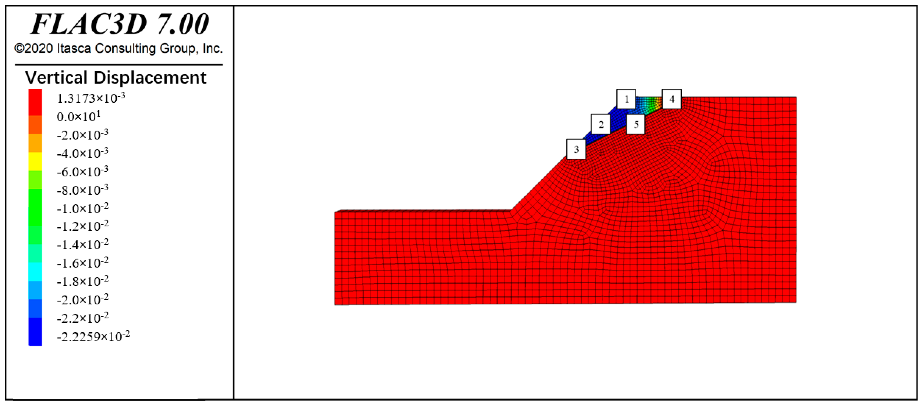
4. Homogeneous Soil Slope (Simple Slope) Stability Analysis Using the FLAC3D Model

A FLAC3D model was constructed to analyze the stability of an 8 m high, 45° inclined, homogeneous soil slope. The slope model consists of 2280 zones and 4794 grid points (Figure 3).

Table 1. Material properties for soil Mohr–Coulomb models.

Parameter	Symbol	Value	Unit
Density	ρ	27	kN/m3
Young’s Modulus	E	12	MPa
Poisson’s Ratio	ν	0.25	-
Cohesion	c	25	kPa
Friction Angle	φ	30	degrees

summarizes the material properties of the homogeneous soil slope. The base of the slope is fixed, while the sides are horizontally constrained. The top is a free boundary. Displacements are monitored at strategic locations—the top, center, toe, and 3.8 m apart horizontally from the slope (Figure 4, Figure 5 and Figure 6), for different modes of contour displacement—horizontal, vertical, and total—are compared across these monitored points (points 1, 2, 3, 4, 5, 6, 7, 8 and 9).

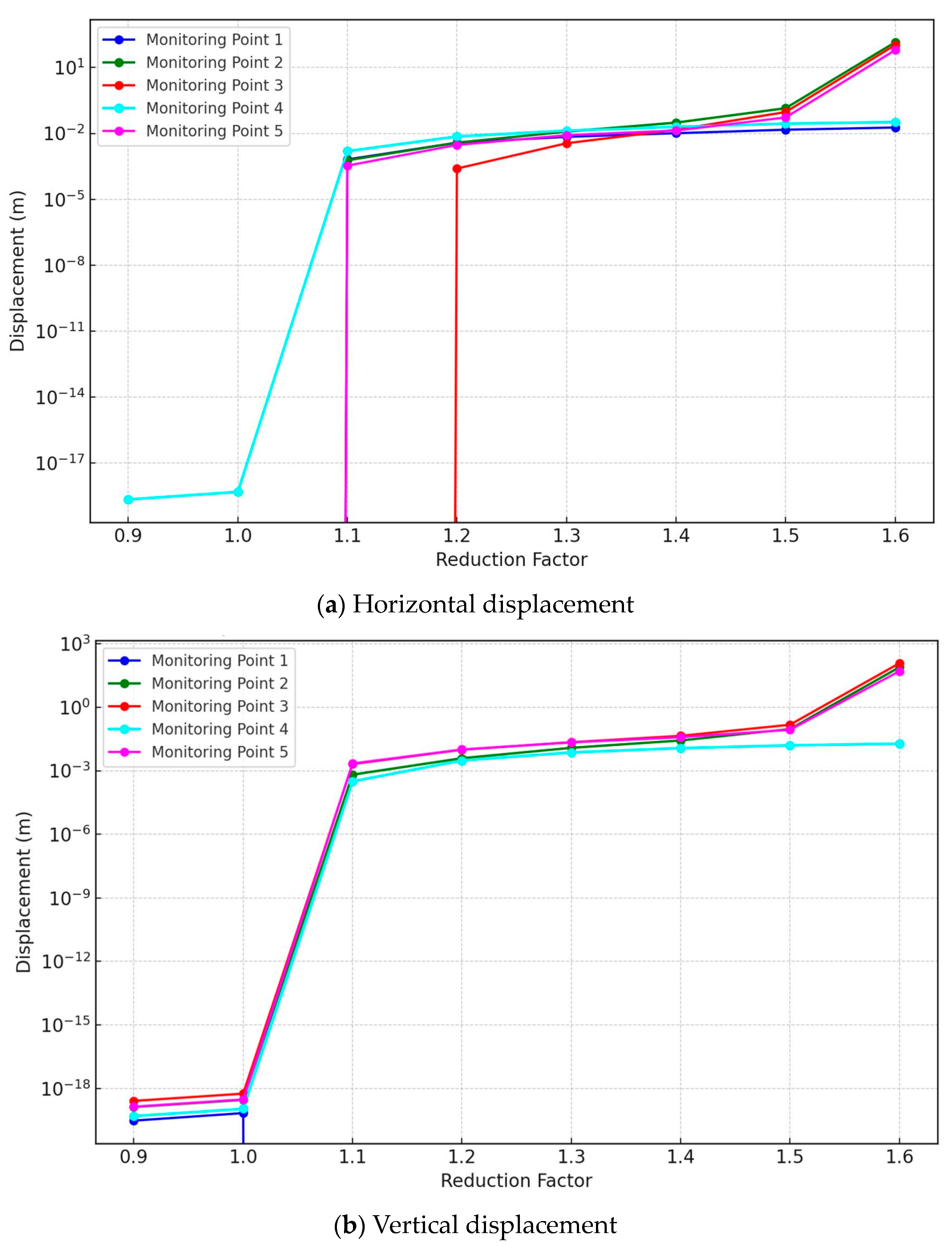
4.1. Analysis of Displacement-Reduction Factor Relationships at Monitoring Points

The relationship between the horizontal, vertical, and total displacements and the reduction coefficient of different monitoring points is recorded, as shown in Figure 7. Also, as can be seen from contour plots, only the displacement curves of points 1, 2, 3, 4, and 5 exist near the boundary slip line, so qualitatively, these points can be considered effective monitoring points with horizontal, vertical, and total displacement positions. The closer the point is to the slope curve, the greater the slope. In some literature, the foot of the slope is chosen as the monitoring point. This is not universal; in this example, the critical slip line does not pass through the foot of the slope, and it cannot indicate whether the slope is damaged or not. Therefore, the position of the slip line is not determined. In this case, it is inappropriate to select the toe of the slope as the monitoring point.

The numerical model displays simulated displacement outputs across monitoring locations and parametric scenarios for a homogenous soil slope stability model. Figure 7a presents the horizontal component of displacements. Positive values represent downslope translations, with magnitudes increasing over higher displacement reduction factors up until instability thresholds are exceeded, indicating translational failures. This is consistent with the findings of Sun et al. regarding the acceleration of horizontal deformations prior to collapse [41]. Figure 7b contains the vertical settlement displacements, with subsidence trends observable leading up to instability thresholds, as highlighted by Zhang et al. regarding precursory deformation [42]. Finally, Figure 7c summarizes the total 3D displacement vectors. At some monitoring points, horizontal translations dominate the failures, while vertical subsidence dominates at other locations—demonstrating spatially heterogeneous modes as analyzed by Call et al.’s geotechnical fragility framework [43,44,45].

4.2. Basic Statistical Properties of Simple Slope

By analyzing each monitoring point separately from

Table 2. Basic statistical properties of simple slope for displacements (horizontal, vertical, and total).

Monitoring Point	Displacement Type	Mean δ (mm)	Standard Deviation δ (mm)	Range δ (mm)
1	Horizontal	0.006846	0.007076	0.0185
2	Horizontal	17.64841	49.84159	141
3	Horizontal	13.26401	37.47101	106
4	Horizontal	0.012809	0.012851	0.0326
5	Horizontal	7.759776	21.91637	62
1	Vertical	−0.00116	0.000966	0.00243
2	Vertical	9.717119	27.42884	77.6
3	Vertical	15.02845	42.41494	120
4	Vertical	0.007152	0.007575	0.019
5	Vertical	6.34475	17.88184	50.6
1	Total	0.006945	0.00711	0.0186
2	Total	20.15416	56.91034	161
3	Total	20.03215	56.55558	160
4	Total	0.014691	0.014899	0.0377
5	Total	10.0222	28.27532	80

, the study recognizes the heterogeneity of slope materials and conditions, resulting in more localized and relevant predictions. The different characteristics between the reduction factor and displacement at each monitoring point highlight the complexity of landslide-triggering mechanisms [46,47,48]. As noted in the analysis, some points show little to no discernible relationship, while monitoring point 2 indicates a potential trend. The minimal displacements and lack of clear correlations at points 1, 3, 4, and 5 suggest that these locations on the slope are likely stable, with marginal changes occurring even under varying stability conditions [48]. This is consistent with Schulz et al., who found that certain areas of a slope can remain unaffected while other sections fail [49]. In contrast, point 2 shows more variability in displacement measurements, which may signal the onset of local ground movement. As discussed by Wright et al., the initiation of slope failure is complex, but increasing deformations suggest changing levels of stability that may precede eventual mass movements [50,51]. The spread in the point 2 data may reflect this early development of failures from additional weight higher up the slope. Overall, these variable strengths and even directions of correlations highlight the heterogeneity of landslide-triggering mechanisms within a slope [49]. Rather than oversimplifying the complexity, site-specific monitoring provides localized insights to better predict zone-specific stability and movement. Targeted early warnings, rather than general alerts, can then be issued when monitoring identifies distinct unstable regions.

Calculating summary statistics such as mean, standard deviation, minimum, and maximum provides quantitative insight into the distribution and spread of displacement readings at each monitoring point [52]. As discussed by Turnbull et al., the mean displacement indicates central tendency, while the standard deviation measures the amount of variation between measurements. A key observation is that monitoring points with higher standard deviations have greater variation in displacement, which correlates with changes in the stability reduction factor [53]. As Crosta and Agliardi explain, increased variability may indicate the early development of movements arising from developing instability. Thus, the statistical dispersion captures subtle effects that are missed by analyzing only the averages [54]. The maximum and minimum displacements also reveal the full dynamic range of variability in the measurements [49]. Defining these endpoints helps to characterize the magnitude of the overall movement currently occurring, even when most measurements are clustered around low means.

Further analysis of exceedance rates and significance tests can build on these descriptive metrics [48]. This statistical characterization provides a quantitative method for systematically tracking changes within slope monitoring data. Rather than just visual assessments, it allows for more definitive comparisons of which sites exhibit the greatest variability, indicating areas of increased risk [54]. The novelty lies in the addition of detailed statistical performance metrics to traditional stability correlations.

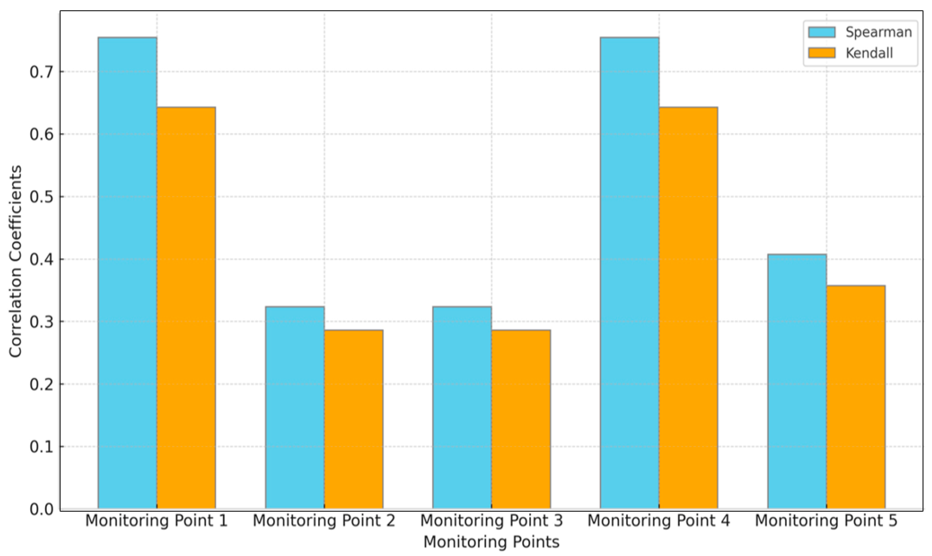
4.3. Spearman and Kendall Correlation Coefficients of Simple Slope

Figure 8, Figure 9 and Figure 10 depict Spearman’s rho correlation coefficients ranging from 0.31 to 0.76, while Kendall’s tau values range from 0.29 to 0.64, indicating variable displacement–stability relationships across the horizontal, vertical, and total displacements. The application of nonparametric Spearman and Kendall correlation coefficients provides a quantitative measure of the monotonic relationship between the reduction factor and displacement values [55]. As explained by Xu et al., these statistical tests assess the strength and directionality of potential correlations between monitoring points [56]. The results show moderately positive but variable correlations in the horizontal, vertical, and total displacements. This is consistent with the work of Travelletti et al., who found that displacement correlations with stability factors can vary significantly depending on the direction and location of the measurement [49]. The variability suggests localization of slope motion rather than broad instability. As highlighted in Crosta and Agliardi, differential displacements suggest that slope failure may begin in isolated sections before spreading [54]. Targeted monitoring helps to characterize these specific unstable zones. Additionally, the mix of positive and weakly correlated data points confirms the complexity of mass movement initiation [56]. Going beyond visual inspection alone, the quantitative correlation coefficients allow for objective comparisons of where destabilization is occurring.

The novelty of this approach is that it complements existing stability indicators with detailed statistical dependence tests. This provides precise, mathematical confirmation of associations across monitored slope locations and measurement directions.

As explained by Xu et al., correlation coefficients (r) range from −1 to +1 and quantify the linear dependence between variables. Values approaching +/− 1 represent strong correlations, while those tending toward 0 indicate weaker or nonlinear relationships [56]. The direction of the association is also crucial. Positive correlations indicate that as one variable increases, the other tends to increase as well. This is consistent with the expectation that greater slope instability (lower reduction factor) promotes higher displacement rates [54]. Negative correlations, on the other hand, imply an inverse relationship between the variables. In this study, the variability in correlation strength and directionality between monitoring locations provides insight into the progression of slope movement. Travelletti et al. found that displacement behavior can vary locally, even on the same slope, under similar conditions. Weak correlations suggest negligible or subtle destabilization effects, while stronger positive correlations are consistent with accelerated zone-specific failures as stability declines [56]. By distinguishing between localized stable and unstable areas through targeted statistical testing, these monitoring data allow for better characterization of the initial progression of slope failures. The displacement correlations can serve as an early warning system, identifying specific regions that warrant greater attention prior to mass failures.

5. Joint Rock Slope Stability Analysis Using the FLAC3D Model

There is a joint plane in the analyzed rock slope. For this joint, a low-strength elastic-plastic sandwich element is used to simulate the joint structure, and the joint inclination angle is 45°, with a thickness of 0.1 m. The rock mass outside the joints is still considered a homogeneous body.

Table 3. Material properties of the rock.

Material	Density (ρ)	Young’s Modulus (E)	Poisson’s Ratio (ν)	Cohesion (c)	Friction Angle (φ)
Layer	29 kN/m3	12 GPa	0.35	600 kPa	37°
Joint	21.5 kN/m3	12 MPa	0.40	12 kPa	20°

summarizes the material properties of the joint rock slope.

The specific dimensions parameters of the slope are shown in Figure 11. The RHINO-FLAC3D interface program was used to establish calculations based on the slope model, and this model has a total of over 4048 units. The lower part of the boundary is fixed, the left and right sides are horizontally constrained, and the upper part is a free boundary. Figure 12, Figure 13 and Figure 14 show different modes of contour displacement—horizontal, vertical, and total—are compared across these monitored points (points 1, 2, 3, 4, and 5).

While the rock and soil slopes have similar contents that are only different in numerical value, the rock has a partly jointed surface, with other parts homogeneous, while the entire soil slope is homogeneous. However, key findings from the soil analysis remain applicable to the jointed rock case. In particular, for both models, monitoring points located outside potential failure surfaces exhibit minimal displacement variations even as stability decreases. This suggests that such points cannot provide advance warning of impending failures. Therefore, the analysis focuses on locations near expected failure zones. However, the presence of joints as persistent weaknesses means that discontinuities have a dominant influence on slope stability. Therefore, the characterization of deformations requires explicit examination of measurements along joint planes, as they may activate prior to global failures. Accordingly, monitoring points were selected at upper, middle, and lower positions along the prominent joint of the slope to profile local variations. For comparison, additional points were monitored away from joints on the slope surface itself. This targeted coverage, along with expected weaknesses, aims to relate measured displacements to stability reductions, given the central role of joints in rock slope evaluation. By distinguishing the behavior of jointed rock while retaining key insights from the homogeneous case, the analysis achieves localized insights into rock mass kinematics while enabling site-specific remediation. Figure 12, Figure 13 and Figure 14 display the horizontal, vertical, and total displacement contours.

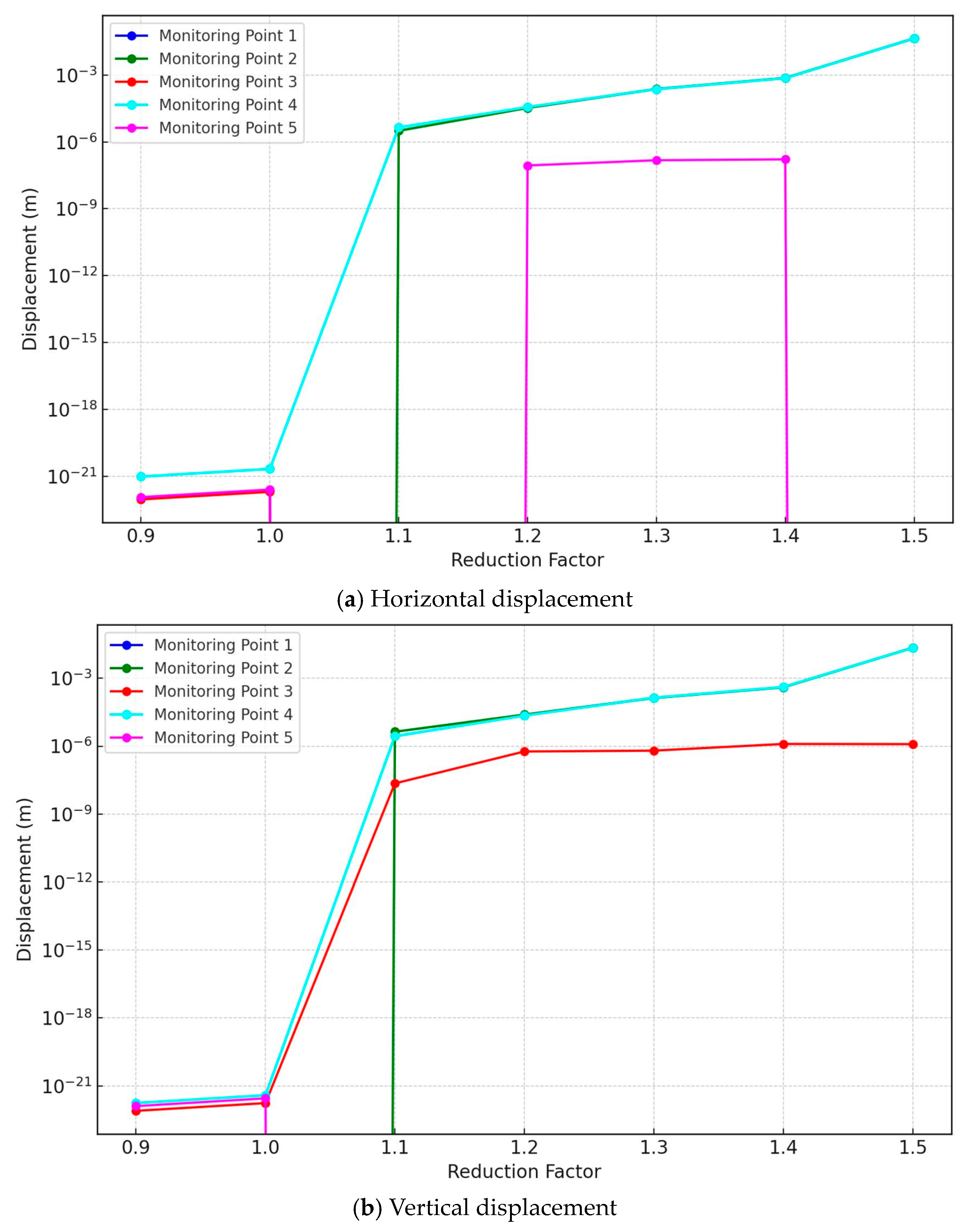
5.1. Analysis of Displacement-Reduction Factor Relationships by Monitoring Point

The simulated displacement results for a parametrically analyzed common rock slope class across monitored locations and displacement directions. Figure 15a shows the isolated horizontal displacements, with initial magnitudes on the order of microns, and drastic downslope displacements occur at points 2 and 4. As noted by Park et al., this is consistent with planar or wedge failures induced along critical discontinuities [57]. Figure 15b then includes the vertical settlement trends, again showing accelerated subsidence at points 2 and 4, while other locations remain relatively stable. The total displacements in Figure 15c confirm concentrated failures governed by translational kinematics. The results demonstrate spatially heterogeneous rupture mechanisms, echoing the fragility concepts of Call et al. [58], while reaffirming the interpretive caution around micron-scale pre-failure deformations, as emphasized by Carlà et al. for early warning systems [59,60,61,62,63].

5.2. Basic Statistical Properties of Joint Slope

Table 4. Basic statistical properties of joint slope for displacements (horizontal, vertical, and total).

Monitoring Point	Displacement Type	Mean δ (mm)	Standard Deviation δ (mm)	Range δ (mm)
1	Horizontal	−6.6 × 10−7	6.1 × 10−7	0.000002
2	Horizontal	0.006448	0.016617	0.044128
3	Horizontal	−3.8 × 10−7	4.15 × 10−7	0.000001
4	Horizontal	0.006469	0.016675	0.044280
5	Horizontal	3.4 × 10−8	1.03 × 10−7	0.000000
1	Vertical	−5.2 × 10−7	4.79 × 10−7	0.000001
2	Vertical	0.003248	0.008346	0.022173
3	Vertical	5.29 × 10−7	5.52 × 10−7	0.000001
4	Vertical	0.003228	0.008291	0.022028
5	Vertical	−7.6 × 10−8	8.36 × 10−8	0.000000
1	Total	8.39 × 10−7	7.75 × 10−7	0.000002
2	Total	0.00722	0.018596	0.049385
3	Total	6.67 × 10−7	6.71 × 10−7	0.000002
4	Total	0.00723	0.018623	0.049456
5	Total	1.16 × 10−7	9.92 × 10−8	0.000000

summarizes the basic statistical properties of horizontal, vertical, and total displacements across monitoring points on the joint slope. As explained by Xu et al., reporting metrics such as mean, standard deviation, minimum, maximum, and quartiles provide a quantitative characterization of the displacement distributions [56]. The data reveal a high degree of variability from point to point. For example, monitoring point 2 has much larger average horizontal and vertical displacements than other locations. Meanwhile, point 5 appears to be the most stable, with consistently negligible displacements. As Crosta and Agliardi noted, slope movements tend to initiate and concentrate locally before spreading. These statistics help to identify emerging unstable zones [54]. In addition, larger standard deviations indicate greater data scatter and variability in measurements over time [56]. For example, monitoring points 2 and 4 show more widespread shifts that may indicate emerging slope instability. The localized insights from statistical testing better inform targeted remediation. Going beyond qualitative observations, numerical profiling of displacement data distributions provides more precise, standardized, and objective comparisons of slope behavior across locations. This augmentation of visual analysis with robust statistical performance metrics improves interpretation and detection capabilities.

5.3. Spearman and Kendall Correlation Coefficients of Joint Slope

Figure 16, Figure 17 and Figure 18 depict Spearman and Kendall correlation coefficients for the joint horizontal, vertical, and total displacements, revealing some compelling insights. Several monitoring points show strong correlations ranges of +1.0 and −1.0. As explained by Uhlemann et al., these values indicate a strong statistical dependence between the stability reduction factor and displacements. The strong positive correlations are consistent with the expectation that decreasing stability corresponds to increasing surface displacements [56]. Conversely, strong negative correlations, such as the horizontal data from point 1, suggest an inverse relationship, where displacements decrease as stability decreases [54]. This deviation from the expected pattern reflects the complexity of slope destabilization. The consistency of very strong positive total displacement correlations implies a predominant overall trend of movement corresponding to deteriorating stability. However, the points still show sufficient variability to avoid overgeneralizing the behavior.

The novelty of this analysis lies in quantifying the local differences in tilt response beyond qualitative observations alone. By documenting the unique correlations, monitoring can better distinguish zone-specific instability progression to design appropriate stabilization interventions.

The major limitations of the study can be summarized as follows: The numerical slope models make significant simplifying assumptions and do not fully capture real-world complexities in terms of soil/rock heterogeneities, hydrogeological factors, weathering effects, etc. In addition, the limited monitoring point coverage provides limited spatial insights, while the micron-scale displacement resolutions pose detection challenges in the field. Furthermore, the limited set of variables and validation data set limitations warrant a cautious application of the presented correlation concepts and failure criteria for field use cases.

To address these limitations, substantial further refinements through integrated physical–numerical modeling and calibrations against instrumented slope case histories are imperative before these simulations can reliably inform early warning methodologies. Specifically, the integration of field measurements, such as slope inclinometers, extensometers, piezometers, rainfall gauges, and topographic surveys, along with laboratory testing of soil and rock samples, would provide a more comprehensive understanding of the slope behavior and failure mechanisms. This combined approach of physical model testing and field calibration is crucial for demonstrating the practical applicability and reliability of the proposed correlation analysis approach for slope stability assessment and landslide forecasting. The authors acknowledge that while the results of the current study illustrate the potential of improved correlation analysis techniques for enhancing landslide prediction capabilities, the methodology requires further validation against real-world data before it can be confidently adopted for operational early warning systems. Comprehensive physical model testing and field calibration are necessary to prove the effectiveness of the proposed approach and its ability to accurately identify critical unstable zones within a slope, thereby informing targeted remediation efforts and early warning strategies.

6. Conclusions

The integration of advanced statistical correlation analysis into slope stability studies represents a significant leap forward in the field of landslide prediction. This novel approach not only improves the accuracy of predictions but also provides deeper insights into the underlying mechanisms of slope failure. As this methodology continues to evolve, it holds the promise of significantly reducing the risks associated with landslides, thereby protecting lives and infrastructure. The following are the key conclusions:

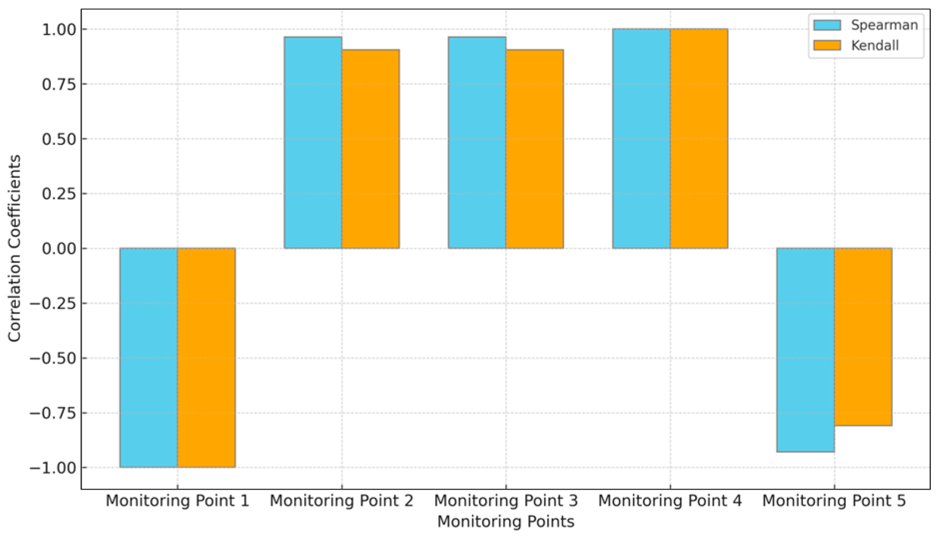
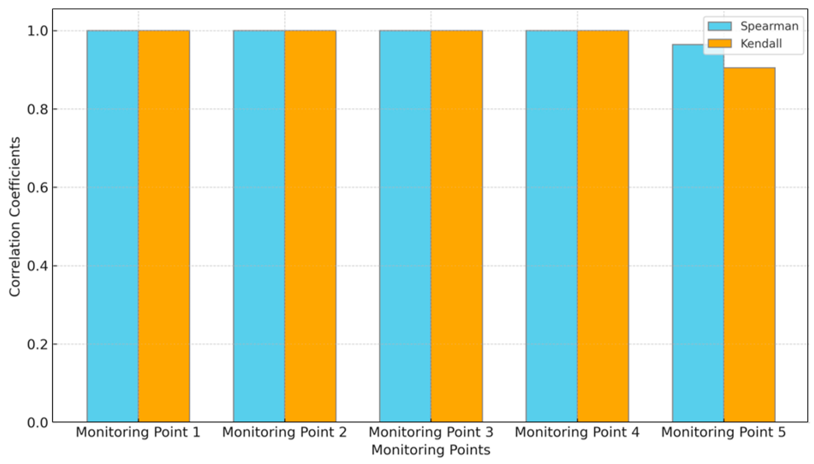
• For the homogeneous soil slope model, the results showed Spearman’s rho correlation coefficients ranging from 0.31 to 0.76, and Kendall’s tau values ranging from 0.29 to 0.64, indicating variable displacement–stability relationships across the monitoring points. In contrast, the joint rock slope model exhibited strong positive total displacement correlations, with Spearman’s and Kendall’s coefficients showing ranges close to +1.0 and −1.0 at most monitoring points. The maximum mean horizontal and vertical displacements reached 44.13 mm and 22.17 mm, respectively, at the critical point 2.
• The quantitative correlation analysis allowed the researchers to identify and distinguish between stable and unstable zones on the simulated slopes, providing localized insights into the progression of slope failures. For example, monitoring point 2 on the soil slope showed a mean horizontal displacement of 17.65 mm and a mean vertical displacement of 9.72 mm under stability reduction, indicating it as a critically unstable location.
• By quantifying the strength and directionality of the correlations between displacement measurements and stability reduction factors, the methodology enables more precise identification of areas prone to instability and potential failure. This level of detail can inform targeted remediation efforts and early warning systems, which is a significant improvement over generalized assessments of overall slope stability.
• Future work should focus on further refinement of the proposed correlation analysis methodology through additional physical model testing and field calibration prior to implementation for early warning systems.

References

1. Elfass, S.A.; Aczel, R.; Norris, G.M.; Jacobson, E. Physical and Numerical Modeling of Rock Joints and Slope Stability. GeoCongress 2006, 2006, 1–6. [Google Scholar]
2. Sun, L.; Liu, Q.; Abdelaziz, A.; Tang, X.; Grasselli, G. Simulating the entire progressive failure process of rock slopes using the combined finite-discrete element method. Comput. Geotech. 2022, 141, 104557. [Google Scholar] [CrossRef]
3. Schneider-Muntau, B.; Medicus, G.; Fellin, W. Strength reduction method in Barodesy. Comput. Geotech. 2018, 95, 57–67. [Google Scholar] [CrossRef]
4. Tu, Y.; Liu, X.; Zhong, Z.; Li, Y. New criteria for defining slope failure using the strength reduction method. Eng. Geol. 2016, 212, 63–71. [Google Scholar] [CrossRef]
5. Umar, I.H.; Lin, H. Marble Powder as a Soil Stabilizer: An Experimental Investigation of the Geotechnical Properties and Unconfined Compressive Strength Analysis. Materials 2024, 17, 1208. [Google Scholar] [CrossRef] [PubMed]
6. Haruna, I.U.; Kabir, M.; Yalo, S.G.; Muhammad, A.; Ibrahim, A.S. Quantitative Analysis of Solid Waste Generation from Tanneries in Kano State. J. Environ. Eng. Stud. 2022, 7, 23–30. [Google Scholar] [CrossRef]
7. Umar, I.H.; Elif, M.; Firat, O. A Study on Uniaxial Compressive Strength and Ultrasonic Non-Destructive Analysis of Fine- Grained Soil in Seasonally Frozen Regions Mevsimsel Donmuş Bölgelerde İnce Taneli Zeminlerin Tek Eksenli Basınç Dayanımları ve Ultrasonik Tahribatsız Analizleri Üzer. Turk. J. Sci. Technol. 2022, 17, 267–677. [Google Scholar] [CrossRef]
8. Umar, I.H.; Firat, M.E.O. Investigation of Unconfined Compressive Strength of Soils Stabilized With Waste Elazig Cherry Marble Powder at Different Water Contents. In Proceedings of the 14th International Conference on Engineering & Natural Sciences, Sivas, Turkey, 18–19 July 2022; pp. 703–711. [Google Scholar]
9. Umar, I.H.; Lin, H.; Ibrahim, A.S. Laboratory Testing and Analysis of Clay Soil Stabilization Using Waste Marble Powder. Appl. Sci. 2023, 13, 9274. [Google Scholar] [CrossRef]
10. Umar, I.H.; Muhammad, A.; Ahmad, A.; Yusif, M.A.; Yusuf, A. Suitability of Geotechnical Properties of Bentonite-Bagasse Ash Mixtures Stabilized Lateritic Soil as Barrier in Engineered Waste Landfills. In Proceedings of the 7th International Student Symposium; Ondokuz Mayiz University: Samsun, Turkey, 2021. [Google Scholar]
11. Umar, I.H.; Muhammad, A.; Yusuf, A.; Muhammad, K.I. Study on the Geotechnical Properties of Road Pavement Failures “(A Case Study of Portion Of Malam Aminu Kano Way, Kano State From Tal-Udu Roundabout To Mambaya House Roundabout)”. J. Geotech. Stud. 2020, 5, 8–15. [Google Scholar] [CrossRef]
12. Chen, W.; Wan, W.; Zhao, Y.; Pen, W. Experimental Study of the Crack Predominance of Rock-Like Material Containing Parallel Double Fissures under Uniaxial Compression. Sustainability 2020, 12, 5188. [Google Scholar] [CrossRef]
13. Wang, H.; Zhang, B.; Mei, G.; Xu, N. A statistics-based discrete element modeling method coupled with the strength reduction method for the stability analysis of jointed rock slopes. Eng. Geol. 2020, 264, 105247. [Google Scholar] [CrossRef]
14. Huang, L.; Lin, H.; Cao, P.; Zhao, Q.; Pang, Y.; Yong, W. Investigation of the Degradation Mechanism of the Tensile MechanicalProperties of Sandstone under the Corrosion of Various pH Solutions. Materials 2023, 16, 6536. [Google Scholar] [CrossRef] [PubMed]
15. Sheikh, M.R.; Nakata, Y.; Shitano, M.; Kaneko, M. Rainfall-induced unstable slope monitoring and early warning through tilt sensors. Soils Found. 2021, 61, 1033–1053. [Google Scholar] [CrossRef]
16. Sztubecki, J.; Mrówczyńska, M. Vertical displacement monitoring using the modified leveling method. Measurement 2023, 206, 112264. [Google Scholar] [CrossRef]
17. Li, H.; Chen, W.; Tan, X. Displacement-based back analysis of mitigating the effects of displacement loss in underground engineering. J. Rock. Mech. Geotech. Eng. 2023, 15, 2626–2638. [Google Scholar] [CrossRef]
18. Hammah, R. ‘Open Secret’ Advantages of the Shear Strength Reduction Approach in Slope Stability Analysis; Rocscience: Sydney, Australia, 2022. [Google Scholar]
19. Krahn, J. Limit Equilibrium, Strength Summation and Strength Reduction Methods for Assessing Slope Stability; GEO-SLOPE International: Calgary, AB, Canada, 2007. [Google Scholar]
20. Hang, L.; Ping, C.; Feng-Qiang, G. Analysis of locations and displacement modes of monitoring points in displacement mutation criteria. Chin. J. Geotech. Eng. 2007, 29, 1435–1438. [Google Scholar]
21. Marchigiani, R.; Gordy, S.; Cipolla, J.; Adams, R.C.; Evans, D.C.; Stehly, C.; Galwankar, S.; Russell, S.; Marco, A.P.; Kman, N.; et al. Wind disasters: A comprehensive review of current management strategies. Int. J. Crit. Illn. Inj. Sci. 2013, 3, 130–142. [Google Scholar] [CrossRef] [PubMed]
22. Intrieri, E.; Carlà, T.; Gigli, G. Forecasting the time of failure of landslides at slope-scale: A literature review. Earth-Sci. Rev. 2019, 193, 333–349. [Google Scholar] [CrossRef]
23. Liu, L.; Zhao, G.; Liang, W. Slope Stability Prediction Using k-NN-Based Optimum-Path Forest Approach. Mathematics 2023, 11, 3071. [Google Scholar] [CrossRef]
24. Chaulagain, S.; Choi, J.; Kim, Y.; Yeon, J.; Kim, Y.; Ji, B. A Comparative Analysis of Slope Failure Prediction Using a Statistical and Machine Learning Approach on Displacement Data: Introducing a Tailored Performance Metric. Buildings 2023, 13, 2691. [Google Scholar] [CrossRef]
25. Chen, F.; Wang, X.-B.; Du, Y.-H.; Tang, C.-A. Numerical analysis of the precursory information of slope instability process with constant resistance bolt. Sci. Rep. 2021, 11, 21814. [Google Scholar] [CrossRef] [PubMed]
26. Barančoková, M.; Šošovička, M.; Barančok, P.; Barančok, P. Predictive Modelling of Landslide Susceptibility in the Western Carpathian Flysch Zone. Land 2021, 10, 1370. [Google Scholar] [CrossRef]
27. Nitsche, M.; Rickenmann, D.; Turowski, J.; Badoux, A.; Kirchner, J. Evaluation of bedload transport predictions using flow resistance equations to account for macro-roughness in steep mountain streams. Water Resour. Res. 2011, 47, 1–21. [Google Scholar] [CrossRef]
28. Wu, X.Z. Trivariate analysis of soil ranking-correlated characteristics and its application to probabilistic stability assessments in geotechnical engineering problems. Soils Found. 2013, 53, 540–556. [Google Scholar] [CrossRef]
29. Hashash, Y.; Song, H. The Integration of Numerical Modeling and Physical Measurements through Inverse Analysis in Geotechnical Engineering. KSCE J. Civ. Eng. 2008, 12, 165–176. [Google Scholar] [CrossRef]
30. Li, Z.; Zhao, X.; Esveld, C.; Dollevoet, R.; Molodova, M. An investigation into the causes of squats—Correlation analysis and numerical modeling. Wear 2008, 265, 1349–1355. [Google Scholar] [CrossRef]
31. Boels, L.; Bakker, A.; Van Dooren, W.; Drijvers, P. Conceptual difficulties when interpreting histograms: A review. Educ. Res. Rev. 2019, 28, 100291. [Google Scholar] [CrossRef]
32. Ozer, M.; Isik, N.S.; Orhan, M. Statistical and neural network assessment of the compression index of clay-bearing soils. Bull. Eng. Geol. Environ. 2008, 67, 537–545. [Google Scholar] [CrossRef]
33. Jambu, M. Chapter 3-1-D Statistical Data Analysis. In Exploratory and Multivariate Data Analysis; Jambu, M., Ed.; Academic Press: Boston, MA, USA, 1991; pp. 27–62. [Google Scholar]
34. Xiao, C.; Ye, J.; Esteves, R.; Rong, C. Using Spearman’s correlation coefficients for exploratory data analysis on big dataset: Using Spearman’s Correlation Coefficients for Exploratory Data Analysis. Concurr. Comput. Pract. Exp. 2015, 28, 3866–3878. [Google Scholar] [CrossRef]
35. Schober, P.; Boer, C.; Schwarte, L. Correlation Coefficients: Appropriate Use and Interpretation. Anesth. Analg. 2018, 126, 1763–1768. [Google Scholar] [CrossRef]
36. Ye, J.; Xiao, C.; Esteves, R.; Rong, C. Time Series Similarity Evaluation Based on Spearman’s Correlation Coefficients and Distance Measures. In Proceedings of the International Conference on Cloud Computing and Big Data in Asia, Huangshan, China, 17–19 June 2015; pp. 319–331. [Google Scholar]
37. Muñoz-Pichardo, J.M.; Lozano-Aguilera, E.D.; Pascual-Acosta, A.; Muñoz-Reyes, A.M. Multiple Ordinal Correlation Based on Kendall’s Tau Measure: A Proposal. Mathematics 2021, 9, 1616. [Google Scholar] [CrossRef]
38. Brossart, D.F.; Laird, V.C.; Armstrong, T.W. Interpreting Kendall’s Tau and Tau-U for single-case experimental designs. Cogent Psychol. 2018, 5, 1518687. [Google Scholar] [CrossRef]
39. Svensson, E. Ordinal invariant measures for individual and group changes in ordered categorical data. Stat. Med. 1998, 17, 2923–2936. [Google Scholar] [CrossRef]
40. Svensson, E. Concordance between ratings using different scales for the same variable. Stat. Med. 2001, 19, 3483–3496. [Google Scholar]
41. Cheng, Q.; Yang, Y.; Du, Y. Failure mechanism and kinematics of the Tonghua landslide based on multidisciplinary pre- and post-failure data. Landslides 2021, 18, 3857–3874. [Google Scholar] [CrossRef]
42. Xia, P.; Ying, C. Research on the stability evaluation method of anchored slopes based on group decision making and matter element analysis. Sci. Rep. 2021, 11, 16588. [Google Scholar] [CrossRef] [PubMed]
43. Jaboyedoff, M.; Del Gaudio, V.; Derron, M.-H.; Grandjean, G.; Jongmans, D. Characterizing and monitoring landslide processes using remote sensing and geophysics. Eng. Geol. 2019, 259, 105167. [Google Scholar] [CrossRef]
44. Luo, H.Y.; Zhang, L.M.; Zhang, L.L.; He, J.; Yin, K.S. Vulnerability of buildings to landslides: The state of the art and future needs. Earth-Sci. Rev. 2023, 238, 104329. [Google Scholar] [CrossRef]
45. Liu, W.; Yan, S.; He, S. Landslide damage incurred to buildings: A case study of Shenzhen landslide. Eng. Geol. 2018, 247, 69–83. [Google Scholar] [CrossRef]
46. Schulz, W.H.; Coe, J.A.; Ricci, P.P.; Smoczyk, G.M.; Shurtleff, B.L.; Panosky, J. Landslide kinematics and their potential controls from hourly to decadal timescales: Insights from integrating ground-based InSAR measurements with structural maps and long-term monitoring data. Geomorphology 2017, 285, 121–136. [Google Scholar] [CrossRef]
47. Lollino, P.; Giordan, D.; Allasia, P.; Fazio, N.L.; Perrotti, M.; Cafaro, F. Assessment of post-failure evolution of a large earthflow through field monitoring and numerical modelling. Landslides 2020, 17, 2013–2026. [Google Scholar] [CrossRef]
48. Stumvoll, M.J.; Schmaltz, E.M.; Kanta, R.; Roth, H.; Grall, B.; Luhn, J.; Flores-Orozco, A.; Glade, T. Exploring the dynamics of a complex, slow-moving landslide in the Austrian Flysch Zone with 4D surface and subsurface information. CATENA 2022, 214, 106203. [Google Scholar] [CrossRef]
49. Muenchow, J.; Brenning, A.; Richter, M. Geomorphic process rates of landslides along a humidity gradient in the tropical Andes. Geomorphology 2012, 139–140, 271–284. [Google Scholar] [CrossRef]
50. Zevgolis, I.E.; Deliveris, A.V.; Koukouzas, N.C. Slope failure incidents and other stability concerns in surface lignite mines in Greece. J. Sustain. Min. 2019, 18, 182–197. [Google Scholar] [CrossRef]
51. Heap, M.J.; Violay, M.E.S. The mechanical behaviour and failure modes of volcanic rocks: A review. Bull. Volcanol. 2021, 83, 33. [Google Scholar] [CrossRef]
52. Cooksey, R.W. Descriptive Statistics for Summarising Data. In Illustrating Statistical Procedures: Finding Meaning in Quantitative Data; Springer: Singapore, 2020. [Google Scholar]
53. Heath, J.P.; Borowski, P. Quantifying proportional variability. PLoS ONE 2013, 8, e84074. [Google Scholar] [CrossRef] [PubMed]
54. Crosta, G.; Agliardi, F. A methodology for physically based rockfall hazard assessment. Nat. Hazards Earth Syst. Sci. 2003, 3, 407–422. [Google Scholar] [CrossRef]
55. Puth, M.-T.; Neuhäuser, M.; Ruxton, G. Effective use of Spearman’s and Kendall’s correlation coefficients for association between two measured traits. Anim. Behav. 2015, 102, 77–84. [Google Scholar] [CrossRef]
56. Mukaka, M.M. Statistics corner: A guide to appropriate use of correlation coefficient in medical research. Malawi Med. J. 2012, 24, 69–71. [Google Scholar] [PubMed]
57. Kettermann, M.; Urai, J. Changes in structural style of normal faults due to failure mode transition: First results from excavated scale models. J. Struct. Geol. 2015, 74, 105–116. [Google Scholar] [CrossRef]
58. Ghalayini, R.; Homberg, C.; Daniel, J.-M.; Nader, F. Growth of layer-bound normal faults under a regional anisotropic stress field. Geol. Soc. Lond. Spec. Publ. 2016, 439, 57–78. [Google Scholar] [CrossRef]
59. Gamperl, M.; Singer, J.; Garcia-Londoño, C.; Seiler, L.; Castañeda, J.; Cerón-Hernandez, D.; Thuro, K. An integrated, replicable Landslide Early Warning System for informal settlements—Case study in Medellín, Colombia. Nat. Hazards Earth Syst. Sci. Discuss. 2023, 2023, 1–16. [Google Scholar] [CrossRef]
60. Han, Y.; Dong, S.; Chen, Z.; Hu, K.; Su, F.; Huang, P. Assessment of secondary mountain hazards along a section of the Dujiangyan-Wenchuan highway. J. Mt. Sci. 2014, 11, 51–65. [Google Scholar] [CrossRef]
61. Zhang, R.; Tang, P.; Lan, T.; Liu, Z.; Ling, S. Resilient and Sustainability Analysis of Flexible Supporting Structure of Expansive Soil Slope. Sustainability 2022, 14, 12813. [Google Scholar] [CrossRef]
62. Zhao, Y.; Liu, Q.; Lin, H.; Wang, Y.; Tang, W.; Liao, J.; Li, Y.; Wang, X. A Review of Hydromechanical Coupling Tests, Theoretical and Numerical Analyses in Rock Materials. Water 2023, 15, 2309. [Google Scholar] [CrossRef]
63. Pang, J.; Xie, J.; He, Y.; Han, Q.; Hao, Y. Study on the Distribution Trend of Rockburst and Ground Stress in the Hegang Mining Area. Sustainability 2023, 15, 9445. [Google Scholar] [CrossRef]
Figure 1. Some structural collapse caused by the landslide on the expressway.
Applsci 14 03685 g001
Figure 2. The flowchart of slope stability analysis using the Strength Reduction Method.
Applsci 14 03685 g002
Figure 3. The soil slope model.
Applsci 14 03685 g003
Figure 4. Location of the monitoring points (contour of horizontal displacement) of soil slope.
Applsci 14 03685 g004
Figure 5. Location of the monitoring points (contour of vertical displacement) of soil slope.
Applsci 14 03685 g005
Figure 6. Location of the monitoring points (contour of total displacement) of soil slope.
Applsci 14 03685 g006
Figure 7. Displacements vs. reduction factor for the existence monitoring points of soil slope.
Applsci 14 03685 g007aApplsci 14 03685 g007b
Figure 8. Correlation coefficients for horizontal displacement of soil slope.
Applsci 14 03685 g008
Figure 9. Correlation coefficients for vertical displacement of soil slope.
Applsci 14 03685 g009
Figure 10. Correlation coefficients for total displacement of soil slope.
Applsci 14 03685 g010
Figure 11. The slope model of the joint rock slope.
Applsci 14 03685 g011
Figure 12. Location of monitoring points (contour of horizontal displacement) of the joint rock slope.
Applsci 14 03685 g012
Figure 13. Location of monitoring points (contour of vertical displacement) of the joint rock slope.
Applsci 14 03685 g013
Figure 14. Location of monitoring points (contour of total displacement) of the joint rock slope.
Applsci 14 03685 g014
Figure 15. Displacements vs. reduction factor for each monitoring point of the joint rock slope.
Applsci 14 03685 g015aApplsci 14 03685 g015b
Figure 16. Correlation coefficients for horizontal displacement of the joint rock slope.
Applsci 14 03685 g016
Figure 17. Correlation coefficients for vertical displacement of the joint rock slope.
Applsci 14 03685 g017
Figure 18. Correlation coefficients for total displacement of the joint rock slope.
Applsci 14 03685 g018