A Comprehensive Review and Tutorial on Confounding Adjustment Methods for Estimating Treatment Effects Using Observational Data

Abstract

Controlling for confounding bias is crucial in causal inference. Causal inference using data from observational studies (e.g., electronic health records) or imperfectly randomized trials (e.g., imperfect randomization or compliance) requires accounting for confounding variables. Many different methods are currently employed to mitigate bias due to confounding. This paper provides a comprehensive review and tutorial of common estimands and confounding adjustment approaches, including outcome regression, g-computation, propensity score, and doubly robust methods. We discuss bias and precision, advantages and disadvantages, and software implementation for each method. Moreover, approaches are illustrated empirically with a reproducible case study. We conclude that different scientific questions are better addressed by certain estimands. No estimand is uniformly more appropriate. Upon selecting an estimand, decisions on which estimator can be driven by performance and available background knowledge.

1. Introduction

Randomized controlled trials (RCT) continue to be the gold standard for evaluating the efficacy and safety of new medical interventions [1]. However, researchers sometimes use observational studies to estimate the effectiveness of treatments and exposures on health outcomes [2]. Direct unadjusted comparisons are misleading when the subjects receiving one treatment differ systematically from the subjects receiving another treatment. For rare diseases, single-arm trials are common due to the impracticability of conducting large randomized trials [3]. Instead, an external control arm is used for comparison under the assumption of no systematic differences across contexts. When there is imperfect compliance, randomized trials no longer estimate the effect of the actual “take up” of a treatment. In per-protocol analyses, the effectiveness of treatments on outcomes can be subject to confounding bias in which those who adhere are systematically different from those who do not; therefore, minimizing potential bias is critical [4,5]. Regulatory agencies have thus issued guidelines for the application of external data in drug development [3,6,7].

There is substantial discussion in the literature regarding estimating the causal treatment effects from observational data via the potential outcome model, in which exchangeability, positivity, and consistency are key assumptions [8,9,10,11,12,13]. Various ways of adjusting covariates are proposed for causal inference to reduce bias and increase precision (i.e., smaller variance) of the estimator, such as the traditional regression models, g-computation, propensity score (PS), and doubly robust approaches [11]. Some researchers have made comparisons for certain methods [13,14]. Ding and Li (2018) [15] provided a systematic review of causal inference from the missing data perspective. However, much of the existing work compares those different methods for a single estimand; therefore, different estimands and the relative performance of various estimators have not been reviewed comprehensively. This work provides a review of common estimands and confounding adjustment approaches. We also discuss bias and precision, advantages and disadvantages, and software implementation for each method.

We start with outlining the causal inference framework and discussing related estimands for different populations in Section 2. Section 3 systematically reviews the most common statistical methods for confounding adjustment. We then briefly discuss diagnosis of checking variable balance in Section 4. An example using real data is then illustrated on how to use various estimators and causal methods with different software tools. This paper then concludes with a brief discussion.

2. Causal Framework and Estimands

Assume that there are $N$ subjects and, for each subject, there is a binary treatment indicator $A_i$ ($i=1,2,\dots ,N$), where $A_i=0$ for the control and $A_i=1$ for the active treatment. The observed endpoint variable is $Y_i$, and $Y_i\left(0\right)$ denotes the potential outcome under the control ($A_i=0$) for subject $i$, whereas $Y_i\left(1\right)$ is for the potential outcome under the active treatment ($A_i=1$). There are $p$ covariates $X_i=\left(X_{i1},X_{i2},\dots ,X_{ip}\right)$ for subject $i$, such as the baseline characteristics, demographic features, risk factors, etc. The covariates can be binary, categorical, or continuous.

The individual treatment effect is the difference between the two potential outcomes for a subject, $Y_i\left(1\right)-Y_i\left(0\right)$. The causal consistency assumption relates an observed outcome to the potential outcome [11].

$$Y_i=A_i{Y}_i\left(1\right)+\left(1-A_i\right)Y_i\left(0\right),$$

which states that the observed response $Y_i$ is equal to the potential outcome with a treatment level that matches the actual treatment level. It is not possible to observe both $Y_i\left(1\right)$ and $Y_i\left(0\right)$ for a single individual. Therefore, the individual treatment effect is not identifiable, and, instead, we focus on the causal effects averaged over subjects.

A commonly used population-level treatment effect is the average treatment effect (ATE), which is defined as the expected individual difference in potential outcomes as below:

$$\mathrm{A}\mathrm{T}\mathrm{E}=E\left[Y\right(1)-Y(0\left)\right].$$

The ATE estimand gives the average effect of treatment in the population and is most relevant when we want to compute an average effect estimate that summarizes the effect for all members in the target population.

The treatment effect may be heterogeneous if it affects individuals differently. In this case, we can divide the population into subsets (e.g., male versus female) and contrast the average effects by subsets. This type of ATE is called the conditional average treatment effect (CATE) and is conditioned on covariates in the subset, as follows:

$$\mathrm{C}\mathrm{A}\mathrm{T}\mathrm{E}=E\left[Y\right(1)-Y(0\left)\right|X=x].$$

In some scenarios, average treatment effects for subpopulations related to treatment are of interest. Two common subpopulations are the subjects in the active treatment group and the subjects in the control group, which are the basis for the average treatment effect for the treated (ATT) and the average treatment effect for the control (ATC), as follows:

$$\mathrm{A}\mathrm{T}\mathrm{T}=E\left[Y\left(1\right)-Y\left(0\right)\right|A=1],$$

$$\mathrm{A}\mathrm{T}\mathrm{C}=E\left[Y\left(1\right)-Y\left(0\right)\right|A=0].$$

ATT is the estimand that is most relevant when we want to evaluate the effect of a treatment among those who are treated, whereas ATC is most relevant when we want to consider the cost incurred by subjects who are not given treatment. The same approaches can be used to estimate the ATT and ATC. For this reason, we only discuss the ATT hereafter.

Moreover, if a matching method is used to pair subjects from the active treatment group to those in the control group, we have a matched subpopulation that may be different from the target (such as the whole or treated) population. The matching approach creates matched sets of treated and untreated subjects who have similar values of PS. The response variable is then compared between the treated and untreated subjects in the matched set. The corresponding estimand is called the average treatment for the matched set (ATM), as follows:

$$\mathrm{A}\mathrm{T}\mathrm{M}=E\left[Y\left(1\right)-Y\left(0\right)\right|M=1],$$

where $M=1$ for matched observations.

Recently, another subpopulation is considered to be of interest, which is the set with the most overlap in the observed covariates between the control and treated [16,17,18]. This subpopulation contains subjects that are eligible to be recruited and assigned to either treatment arm with a similar probability, and thus may more closely mimic a population enrolled in a RCT [17]. The estimand for the overlap population is called ATO (Web appendix of Li et al. [18]):

$$\mathrm{A}\mathrm{T}\mathrm{O}=\frac{E\left[e\left(X\right)\left(1-e\left(X\right)\right)\left(Y\left(1\right)-Y\left(0\right)\right)\right]}{E\left[e\left(X\right)\left(1-e\left(X\right)\right)\right]},$$

where $e\left(X\right)$ is the propensity score, i.e., the probability of a subject being assigned to the active treatment arm given the covariates, $e\left(X\right)=\mathrm{P}\mathrm{r}(A=1|X=x)$.

The choice of estimand(s) will depend on the research objectives. If the research question is about the effect on outcomes for all subjects, then the ATE is likely the best choice. If the research goal is to evaluate the effect on outcomes among subjects who received the active treatment, then the ATT would be most appropriate. If the research interest is regarding the subpopulation of those who have equal probability to be in either the active treatment or control group (e.g., the randomized controlled trial), then ATO is the best option.

3. Confounding Adjustment Methods

Once the estimand is selected, the next task is to express the estimand in terms of the observed data, referred to as ‘identification’. Identification often relies on the assumptions of causal consistency and exchangeability (or ignorability) with positivity [19,20]. As described above, the causal consistency assumption links the potential outcomes to the observed outcomes. Exchangeability stipulates that the potential outcomes and treatment are independent marginally or conditionally. Conditional exchangeability is mathematically expressed as $E\left[Y\left(a\right)|X\right]=E\left[Y\left(a\right)|A=a,X\right]$ for all values $a$ of treatment. In other words, exchangeability is the assumption that there are no unobserved common causes of the exposure and outcome. For exchangeability to be mathematically well defined, we further assume that the probability of receiving a treatment is non-zero for every covariate combination relevant for exchangeability. This assumption is referred to as positivity and written as $\mathrm{Pr}\left(A=a|X\right)>0$ [21].

In an RCT, marginal exchangeability is met by design and covariates are balanced in expectation. However, chance imbalances can still occur, particularly when a sample size is small. Accounting for chance imbalances by covariates strongly predictive of the outcome can provide more precise estimates of causal effects [22]. Here, the goal of covariate adjustment is to improve precision and power in estimating causal effects.

If a study is not randomized, there can be systematic imbalance in covariates for different treatment arms (i.e., marginal exchangeability does not hold). Instead, one can assume there is a sufficient adjustment set for confounding (i.e., conditional exchangeability). Confounding adjustment can then be achieved via different ways, such as traditional outcome regression, g-computation, PS adjustment, and doubly robust approaches.

Outcome regression methods were first developed to estimate conditional effects accounting for covariate imbalance between treatment arms [23,24]. However, standard adjustment by parametric regression models is sensitive to model mis-specification [8]. G-computation has been proposed as a way to estimate the marginal causal effect using an outcome regression model [25]. G-computation allows for a treatment effect to be different for different levels of the covariates, and it is also relatively robust to model mis-specification if there is no unmeasured confounding [26]. Alternatively, propensity score (PS) methods that use PS in different ways to control confounding include matching [10,27], stratification [28,29], weighting, and conditional adjustment using PS as a covariate [30]. For example, the inverse probability weights (IPW) can be applied to subjects in each treatment arm to balance the covariate distributions, and the comparison is made between the weighted outcomes [17,23,31,32,33,34]. Researchers [35] used a few large-scale cardiovascular observational studies to compare the performance of a conventional regression with PS methods. PS is the most widely applied causal inference tool for observational studies and it has theoretical advantages over conventional confounding adjustment using outcome regression. Another option is the doubly robust approach that combines PS methods and outcome regression. One of the doubly robust methods is the augmented IPW estimator, which can provide unbiased estimates if one of the models is mis-specified. We discuss each approach in more detail below.

3.1. Traditional Regression

For traditional regression, a model is fit for the response $Y$ on the treatment indicator $A$, covariates $X$, and sometimes their interactions $A\ast X$. For example, a multiple linear regression for a continuous endpoint is set up as

$${\mathrm{Y}}_i={\beta }_0+{\beta }_1{A}_i+{\beta }_2{X}_{1i}+{\beta }_3{X}_{2i}+\cdots +{\epsilon }_i,$$

where $({\beta }_0,{{\beta }_1,\beta }_2,\dots )$ are the regression coefficients and ${\epsilon }_i$ is the random error. The least square estimator of ${\beta }_1$ can be taken as the estimator of CATE.

A logistic regression for a categorical endpoint is constructed as

$${\mathrm{l}\mathrm{o}\mathrm{g}\mathrm{i}\mathrm{t}\left[\mathrm{P}\mathrm{r}\right(\mathrm{Y}}_{\mathrm{i}}|A_i,X_i)]={\beta }_0+{\beta }_1{A}_i+{\beta }_2{X}_{1i}+{\beta }_3{X}_{2i}+\cdots .$$

The difference $\mathrm{P}\mathrm{r}(\mathrm{Y}=1\left|A=1,X=x\right)-\mathrm{P}\mathrm{r}(\mathrm{Y}=1|A=0,X=x)$ can be used as the estimator of CATE when $X=x$.

One concern of fitting a logistic regression is that the number of covariates may be very large compared to the number of events when the event of interest is rare. The rule of thumb is to have at least 10 events of the endpoint for each covariate in the regression, but that rule can be relaxed [36]. The regression model further assumes that the treatment effect measure is constant across the levels of covariates (or confounders) included in the model, but this is not often expected to be the case. Model mis-specification may lead to bias and impact precision in unbalanced designs with treatment effect heterogeneity [37]. With non-linear models, like logistic regression, the coefficient of treatment may not represent the marginal effect due to non-collapsibility [38]. For parameters such as odds ratios (OR), the subgroup-specific conditional treatment effects may be different from the unconditional treatment effect, even in the absence of confounding bias.

3.2. G-Computation

In 1986, a paper by Greenland and Robins demonstrated that, under the previous identification assumptions, a consistent estimate of the unconditional treatment effect can be obtained by using the g-computation formula [26,38,39]. G-computation is a generalization of standardization with respect to the covariates’ distribution. G-computation takes the model from traditional regression and computes $\mathrm{P}(Y=1|A=1,X_i)$ and $\mathrm{P}(Y=1|A=0,X_i)$ for all subjects, which are the two predicted probabilities of events for a subject’s covariates vector $X_i$ under both treatment and non-treatment. These predications can then be used to estimate the reviewed estimands by taking the corresponding mean. For ATE, we include all subjects in the prediction set; for ATT, only treated subjects are included. G-computation, based on the estimation of the components, allows for a treatment effect to vary by different covariates. More in-depth walkthroughs of how g-computation is applied can be found in the following references [14,39]. G-computation is fairly robust in regard to model mis-specification for estimating the marginal (or adjusted population-averaged) risk difference if there is unmeasured confounding is not an option [38,40].

3.3. Propensity Score Methods

Propensity score (PS) methods are increasingly popular in observational studies as an alternative to traditional covariates adjustment via a regression model. PS is one of the most frequently used causal inference methods [9]. The PS methods are a set of statistical tools that seek to balance non-equivalent groups with non-randomized designs. Simply speaking, an individual’s PS is their probability to have received a treatment conditional on a set of covariates, i.e., $e\left(X\right)=\mathrm{P}\mathrm{r}(A=1|X=x)$. PS is commonly estimated by the standard logistic regression model. Other methods, such as nonparametric regression, generalized additive models, and machine learning methods, can be used to improve PS estimation [41].

In a randomized trial, the true PS is known by design, whereas, in an observational study, the PS must be estimated. The PS is typically estimated through a logistic regression that incorporates variables that are associated with treatment assignment. Because the PS summarizes all covariates as a single PS variable, it is able to mitigate problems of overfitting for the outcome model [35,42]. The PS approach would not help much if the outcome model is linear; however, tut the PS estimation may reduce overfitting for binary outcome models (especially with rare diseases), as the PS summarizes all other covariates into a single variable for the outcome model. Since the treatment assignment between the active and the control is often well balanced (which is relatively common in practice), one can flexibly model many covariates in the PS model. After the PS scores have been obtained, we use them to estimate the treatment effect. PS-based approaches separate the design and analysis in the sense that the PS model can be developed using only data regarding the covariates and treatment variables. Excluding the outcome from development of the PS estimation can avoid the “fishing expedition” of fitting models until favorable results are obtained [38].

There are various methods of using PS for estimating treatment effects: (1) matching; (2) stratification; (3) weighting; (4) using PS as a covariate in an outcome regression.

3.3.1. PS Matching

This approach creates matched sets of treated and untreated subjects with close PS values. The matching ratio can be different, with one-to-one pair matching being the most common. The response variable then is compared between the treated and untreated subjects in the matching set. The matching can be with or without replacement, and each untreated subject is paired to only one treated subject in matching without replacement, while each untreated subject can be matched to more than one treated subject in matching with replacement. Two common methods of matching are optimal matching and greedy matching. Optimal matching involves forming matched pairs to minimize the average within-pair difference in the PS. Greedy matching selects treated subjects sequentially for matching. For a given treated subject, select the closest untreated subject, even if that untreated subject would better serve as a “match pair” for a subsequent treated subject. Gu et al. [43] compared these two matching methods, concluding that optimal matching performed no better than greedy matching in producing balanced matched samples.

3.3.2. PS Stratification

PS stratification divides a dataset into several strata based on PS scores. A treatment effect is studied in each stratum and an overall treatment effect is computed using a weighted average across all strata. This method compares the outcome between treated and untreated subjects who are similar in their PS and thus also likely to be similar in the distribution of their measured covariates. Stratification uses weights that are proportional to the number of subjects in each stratum and allows for estimating the average treatment effect. The weight is $1/k$ when there are $k$ equal strata. The ATT can be estimated if we weight by the stratum-specific number of treated subjects, while the ATE is estimated if we weight by the sum of stratum-specific numbers of treated and control subjects [28,29].

3.3.3. PS Weighting

PS weighting is another important tool in causal inference that can be implemented in different ways.

(1)

Inverse Probability of Treatment Weighting (IPTW)

By IPTW, subjects are weighted by the inverse probability of being assigned to the treatment: $w_i=\frac{A_i}{e_i}+\frac{1-A_i}{1-e_i}$. However, we often need to estimate the weights in observational studies, so $e_i$ would be estimated. Additionally, notice that weights can become quite large when $e_i$ is near zero. For variance estimation, the distinction between the known weights and estimated weights is important [32]. The covariate imbalance between treatment groups is reduced by the weighting approach, and so an outcome can be compared directly between treated and untreated subjects in the weighted data. The IPTW can be used to estimate the ATE (

Table 1. Summary of various types of population, corresponding estimands, and weights for both treated and control subjects.

Population	Estimand	Weight
Combined	ATE	$w_1=\frac{1}{e_i\left(x\right)},w_0=\frac{1}{1-e_i\left(x\right)}$
Treated	ATT	$w_1=1,w_0=\frac{e_i\left(x\right)}{1-e_i\left(x\right)}$
Overlap	ATO	$w_1=1-e_i\left(x\right),w_0=e_i\left(x\right)$
Matchable Treated	ATM	$w_1=\frac{\min \left\{e_i\left(x\right),1-e_i\left(x\right)\right\}}{e_i\left(x\right)},$
		$w_0=\frac{\min \left\{e_i\left(x\right),1-e_i\left(x\right)\right\}}{1-e_i\left(x\right)}$

).

(2)

ATT Weighting

Alternate weighting $w_i=A_i+\frac{(1-A_i)e_i}{1-e_i}$ is used to obtain ATT, that is $w_i=1$ when a subject is in the treatment group and $w_i=\frac{e_i}{1-e_i}$ when a subject is in the control group (Table 1). A key requirement for both IPTW weighting and ATT weighting is the positivity assumption, meaning that PS should not be too close to 0 or 1. When this assumption fails, a small number of highly influential weights may lead to unstable weighting estimators. A few alternative methods have been proposed, including trimming and the overlap weighting [44].

(3)

Overlap Weighting (OW)

The overlap weight is the probability that a subject is assigned to the opposite group, i.e., ${1-e}_i$ for a subject in the treated group and $e_i$ for a subject in the control group. The OW focuses on the causal effects on the population with the most overlap in covariates between two treatment groups [18]. Estimation under unconfounded or ignorable treatment assignment is often hampered by a lack of overlap in the covariates, which may result in imprecise estimates and lead to estimators that are sensitive to the choice of specification. The OW procedure involves the following a few steps: (1) estimating the $e_i$ from a model; (2) calculating the weights based on the estimated PS: ${\widehat{w}}_1=1-{\widehat{e}}_i\left(x\right)$ if in the treatment group and ${\widehat{w}}_0={\widehat{e}}_i\left(x\right)$ if in the control group; (3) normalizing the weights so that the sum of the weights equals 1 within each group; (4) estimating the average treatment effect for the overlap population by the difference of the OW-weighted average outcomes between the groups.

Compared to the traditional IPTW weights and associated trimming methods, OW has several advantages: (1) there are no extreme weights; (2) it gives minimum variance of the weighted estimator of causal effects among all balancing weights (including IPTW); (3) the exact mean balance of covariates is achieved when PS is estimated via a logistic regression; and (4) there is no need to choose an artificial cutoff point, as required by trimming.

3.3.4. Use PS in Regression

Rosenbaum and Rubin [9] suggest to add the PS term in the regression model. For example, the estimated PS term ($\widehat{e}\left(X_i\right)$) is added into a linear regression model:

$$Y_i={\beta }_0+{\beta }_1{A}_i+{\beta }_2\widehat{e}\left(X_i\right)+{\epsilon }_i,$$

where $A_i$ indicates the treatment assignment for subject $i$ and ${\beta }_1$ is the treatment effect conditional on the PS values that are calculated based on the covariates.

3.4. Doubly Robust Estimator

Doubly robust estimators combine models for the treatment and outcome in such a way that they provide unbiased estimates for the treatment effect as long as one of the models is correctly specified. Augmented Inverse Probability Weighting (AIPW) is a commonly used doubly robust estimator. The AIPW is built by combing an inverse probability weighting approach with g-computation [45]. For each treatment group, a separate model for the outcome variable is fitted by using a set of covariates, and the potential outcomes that correspond to each treatment assignment are predicted for all the subjects as follows:

$${\widehat{Y}}_i\left(0\right)=g^{-1}\left(X_i\widehat{{\mathit{\beta }}_c}\right),{\widehat{Y}}_i\left(1\right)=g^{-1}\left(X_i\widehat{{\mathit{\beta }}_t}\right)$$

where $g^{-1}$ is the inverse link function used in the generalized linear model for the outcome variable, $\widehat{{\mathit{\beta }}_c}$ is the regression coefficient estimate for the outcome regression model in the control group, and $\widehat{{\mathit{\beta }}_t}$ is the coefficient estimate for the outcome regression model in the treatment group. The AIPW estimates are given by [46]

$${\widehat{\mu }}_0=\frac{1}{n}\sum _{i=1}^n\frac{(1-A_i)Y_i}{1-\widehat{e_i}}+\frac{\left(A_i-\widehat{e_i}\right)}{1-\widehat{e_i}}{\widehat{Y}}_i(0),$$

$${\widehat{\mu }}_1=\frac{1}{n}\sum _{i=1}^n\frac{A_i{Y}_i}{\widehat{e_i}}-\frac{\left(A_i-\widehat{e_i}\right)}{\widehat{e_i}}{\widehat{Y}}_i(1),$$

where $\widehat{e_i}$ is the predicted PS for a subject from the treatment model.

A targeted maximum likelihood estimator (TMLE) is another doubly robust estimator that is based on a targeting step to optimize the bias-variance tradeoff for the parameters of interest [47]. Like the g-computation, TMLE estimates the predicted probabilities of potential outcomes for each subject. Then, g-computation calculates the difference in those two predicted probabilities over all levels of the covariates, whereas TMLE involves an extra targeting step incorporating the inverse probability weights prior to calculation of treatment difference.

4. Diagnostics of Covariate Balance

We outline the methods used for assessing balance in covariates suggested in Zhang et al. [48]. These diagnostics compare whether the distributions of relevant covariates are similar between the treated and untreated subjects [30,49].

The common measures of balance include the standardized differences and comparison of the distributions of covariates. The standardized mean difference (SMD) is defined as

$${\mathrm{S}\mathrm{M}\mathrm{D}}_{1vs0}=\frac{|\overline{X_1}-\overline{X_0}|}{\sqrt[2]{(S_1^2+S_0^2)/2}},$$

where $\overline{X_1},\overline{X_0}$ are the sample means of the covariate for the two arms and $S_1^2$, $S_0^2$ are the corresponding sample variances. The SMD for the dichotomous variable is

$${\mathrm{S}\mathrm{M}\mathrm{D}}_{1vs0}=\frac{|\overline{p_1}-\overline{p_0}|}{\sqrt[2]{\left(\overline{p_1}\right(1-\overline{p_1})+\overline{p_2}(1-\overline{p_2}\left)\right)/2}},$$

where $\overline{p_1},\overline{p_0}$ are the sample proportions for the two treatment arms. This formula can be extended for categorical variables where the comparison can be employed at each level of the variable or the Mahalanobis distance can be used, as proposed by Dalton [50]. SMD is interpreted as the mean difference in a unit of the standard deviation and does not depend on sample sizes or units of the variable that is measured. Because SMD does not depend on the measurement unit, it allows for comparisons between variables with different units. SMD is often presented with a love plot that graphically displays a covariate balance before and after adjusting. Generally, 0.1 represent reasonable SMD thresholds for balance [48]. Other common balance measures include the Kolmogorov–Smirnov (KS) test statistics and t-statistics [51]. Variance is the second central moment of the mean and should also be compared. A variance ratio of 1 between treatment groups indicates a good balance, and a variance ratio between 0.5 and 2 is generally acceptable [48].

Moreover, we can look at the interactions, higher order terms, etc. The standard distribution tests can be employed, such as empirical cumulative distribution functions or non-parametric estimates of the density function of each covariate. Simple plotting, such as with side-by-side boxplots, Q-Q plots, and residual plots, is helpful and convenient.

Prognostic scores, defined as the predicted probability of the outcome in the control, can be used for assessing balance as well [52]. We can first regress the response on covariates only in the control group; then, that fitted model is employed to predict an outcome for all subjects. Simulation study has shown that the prognostic score approach can outperform mean differences and significance tests for assessing balance [52].

5. Software Tools for Implementation

Several software programs that implement confounding adjustment are available in many programming languages, including R, Python, SAS, and Stata. There are a number of R packages for PS methods, including twang [53], CBPS [54], PSW [55], ATE [56], WeightIt [57], causalweight [58], sbw [59], and PSWeight [60], as well as several packages that implement doubly robust estimators, including AIPW [61], CausalGAM [62], npcausal (nonparametric causal inference) [63], and tmle (targeted maximum likelihood estimation) [64]. The Comprehensive R Archive Network (CRAN) task view for causal inference provides a list of many more packages related to this topic [65]. Some packages are available in Python, such as zEpid [66], delicatessen [67], and PyWhy [68]. SAS provides many procedures for general confounding adjustment, such as PSMATCH, LOGISTIC, CAUSALGRAPH, CAUSALMED, and CAUSALTRT [46,69]. These causal procedures can be used to calculate PS, produce matched sets, estimate various estimands, and assess covariate balance. There are many ways of calculating standard errors in causal inference. The CAUSALTRT Procedure in the SAS/STAT^® 15.3 User’s Guide provides details and formulas for standard errors and confidence intervals [69]. Ding [13] gives good coverage of obtaining standard errors for various estimators.

6. Example

This example uses the Study to Understand Prognoses and Preferences for Outcomes and Risks of Treatment (SUPPORT), which was a multi-center observational study on seriously ill and hospitalized patients to examine the effectiveness of Right Heart Catheterization (RHC) in the initial care of critically ill patients [70]. The dataset pertains to Day 1 of hospitalization. This example includes all 5735 subjects who were admitted to an ICU in the first 24 h after entering the study. RHC was coded as present if it was performed, and there were 2184 patients who received RHC. The outcome of interest is patients’ chance of surviving by the end of first month. The original analysis by Connors et al. [70] used a binary logistic model to obtain PS to match RHC patients with No-RHC patients. Their results provided evidence that RHC patients had a decreased survival time.

Here, we apply the reviewed methods (i.e., regression with all covariates, g-computation, weighting, stratification, matching, and AIPW) and describe important steps for their implementation. In the Supplementary document, we provide code to replicate the analyses.

All the covariates (~50) are included, as suggested by Connors et al. [70]. The logistic regression is used to determine the PS, i.e., the probability of receiving RHC for each subject. The effectiveness of using PS to account for major covariates’ imbalance is tested for differences between the two RHD groups (with and without RHC).

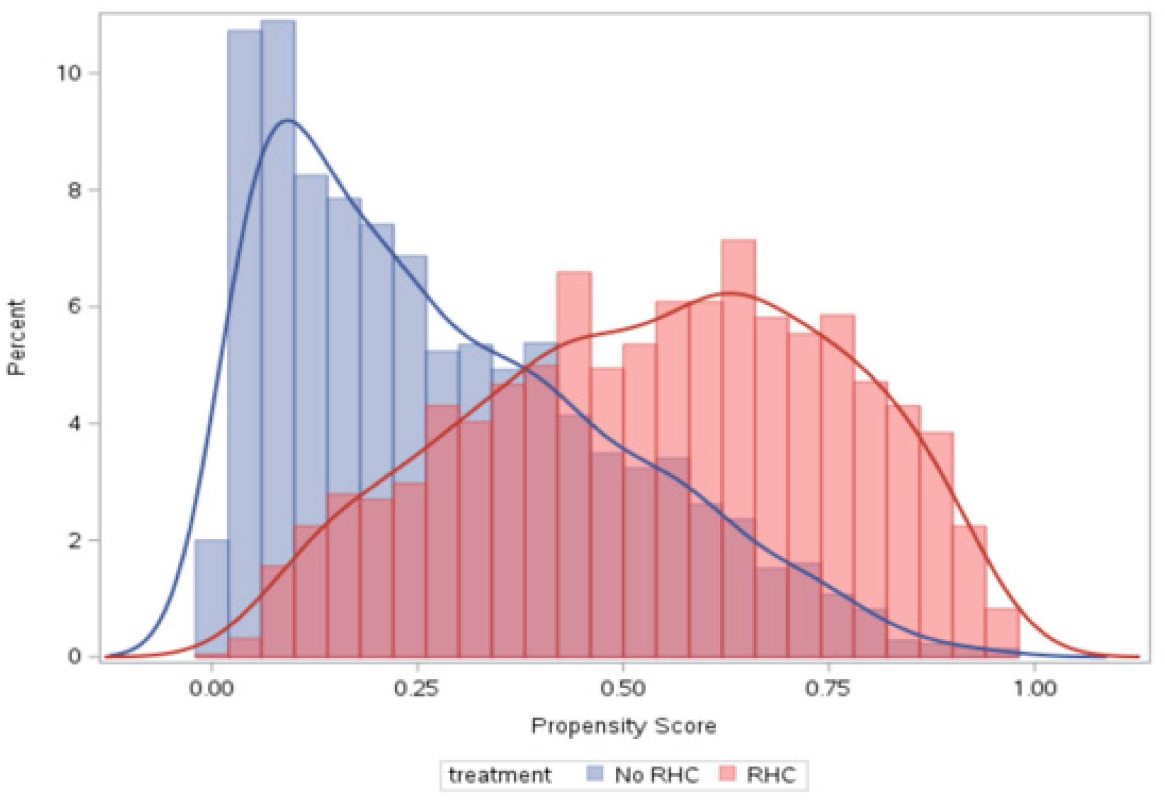
The PS distributions for the two RHD groups are displayed in Figure 1. The graph shows apparent differences in the PS distributions. There are many subjects with small PS values (around 0) and large ones (close to 1), indicating some covariate combinations were highly predictive of receiving RHC. The patients whose PS and RHC status do not agree may be atypical but received large weights.

The love plot in Figure 2 compares the standardized differences of selected covariates included in the PS model: (1) blue for the original data in the regular regression; (2) purple for ATT weighting; (3) red for ATE weighting; (4) black for matching; (5) green for overlap weighting. We can see that the mean differences for most covariates are quite large in the traditional regression but are reduced with the adjustment methods. For all the methods, the largest SMD in absolute value is less than the recommended limit of 0.1 [48]. These indicate the effect of those methods on reducing the differences in covariates. The SMD with overlap weighting is the smallest (very close to zero in green). PS matching and weighting seem to remove a greater portion of systematic differences between the treated and untreated subjects compared with many other approaches, such as stratification and traditional regression, which is in agreement with Peter Austin’s 2009 paper [71]. Among weighting approaches, overlap weighting seems to perform the best in terms of having the smallest mean difference, as expected.

The endpoint was surviving up to one month post-ICU admission. A binomial model with the logit link is used to obtain the risk difference and odds ratio for comparing the treatment effect of RHC versus No-RHC. We present the point estimates on the risk difference, standard errors, p-values, and corresponding confidence intervals for various methods. The results are displayed in

Table 2. Analysis results for the binary outcome of passing the first month: The point estimates on risk difference in having 30-day mortality between RHC and No-RHC groups, associated standard errors, p-values, and confidence intervals for various methods. All methods except for the crude model include all available covariates.

Estimand	Methods	Risk Difference	Standard Error	p-Value	95% CI of Risk Difference
Crude	Regression without covariates	0.074	0.013	<0.0001	[0.048, 0.099]
CATE	Traditional regression with all covariates	0.072	0.021	<0.0001	[0.031, 0.114]
ATE	G-computation	0.059	0.014	<0.0001	[0.032, 0.087]
	PS stratification (5 strata)	0.055	0.032	0.1622	[−0.008, 0.119]
	PS weighting: IPTW	0.053	0.010	<0.0001	[0.035, 0.070]
	Doubly robust	0.059	0.014	<0.0001	[0.032, 0.087]
ATT	G-computation	0.056	0.014	<0.0001	[0.028, 0.085]
	PS stratification (5 strata)	0.055	0.030	0.1623	[−0.008, 0.118]
	PS weighting	0.053	0.014	<0.0001	[0.025, 0.081]
	Doubly robust	0.062	0.016	<0.0001	[0.029, 0.094]
ATM	PS matching	0.049	0.017	0.0035	[0.016, 0.08]
ATO	Overlap weighting	0.057	0.012	<0.0001	[0.031, 0.083]
	Overlap weighting with doubly robust	0.059	0.012	<0.0001	[0.033, 0.085]

Note: The results from using SAS are presented whenever there is a suitable procedure available to use in SAS. For the doubly robust estimator for ATT and overlapping weighting, the PSWeight package in R was used.

, where the content is first arranged by the type of estimands, then by confounding adjust methods. In the Estimand column, we list the crude effect estimate, ATE, ATT, ATM, and ATO. For the crude effect, no covariates were included in the logistic model except for the treatment variable, and SAS’s LOGISTIC procedure was used. For ATE, many methods were implemented, including the traditional regression with all covariates (SAS LOGISTIC), g-computation (SAS CAUSALTRT), PS stratification (SAS PSMATCH), PS weighting (SAS PSMATCH), and doubly robust estimators (SAS CAUSALTRT, the AIPW and PSWeight packages in R). For the remaining ATT, ATM, and ATO estimands, almost all estimators were employed as well. In Table 2, the results from using SAS are presented whenever there is a suitable procedure available in SAS, with the exception that the PSWeight package in R is used for the doubly robust estimator for ATT and overlapping weighting.

The crude estimate, without accounting for any covariates, and the CATE with a traditional regression, accounting for all covariates, give relatively larger risk differences (0.074 and 0.072, respectively) compared to most other methods (0.050–0.059). Most other methods, such as g-computation, PS weighting, etc., produce similar results in terms of having comparable point estimates and confidence intervals. The risk difference between the RHC and No-RHC control groups is all positive, indicating that patients with RHC had an increased rate of 30-day mortality after adjusting for treatment selection bias. This result confirms with the original analysis by Connors et al. that RHC patients had decreased survival rates compared to No-RHC patients [70].

PS stratification can be unstable when the number of strata is large or the data size is small. In this example, stratification with five strata showed some signs of instability, with the first stratum and the last stratum having a relatively large standard error; additionally, it would be even worse in terms of having estimates that are very different from stratum to stratum when the number of strata increases to 10.

The ATM risk difference obtained from the matched observations is the smallest (0.049), proving to be a little different than most ATE and ATT estimates. This is because ATM represent the matched observation pool, a subset of the whole population that most ATE and ATT is derived from.

In general, it seems that the ATO with overlap weighting and its doubly robust version have the smallest standard errors and, therefore, the smaller confidence intervals, as claimed in Li et al. [17]. However, the performance of any method must be considered in terms of the estimand and that estimand’s relevance to the motivating scientific question.

7. Discussions

In randomized control trials, it is reasonable to assume there are no systematic differences in covariates between treatment groups. Therefore, the causal effect of a treatment can be directly estimated by comparing the observed outcome in the active treatment group versus that in the control group. To evaluate the treatment effect from observational data, additional effort must be made to remove the impact of confounding variables, which are related to both the treatment and outcome.

For observational data, making causal inference needs to elect an appropriate estimand to start. The choice of estimands relies on the research objectives. For example, if we want to make an inference about the effect on outcomes for all subjects, then the ATE should be the preferred estimand. If the population of interest is among subjects who selected treatment, then the ATT should be used. If one is interested in comparing causal effects estimated from an observational study to that from a randomized trial, then ATO might be more appropriate.

We reviewed a wide range of confounding adjustment methods. Each method has its own pros and cons.

Table 3. Comparison of different confounding adjustment methods.

Method	Advantage	Disadvantage
Traditional regression	Simplest and easy to fit Provides a prognostic model for outcome of interest	Model mis-specification decreases precision in unbalanced design May be implausible with a large number of covariates Treatment effect is assumed to be the same for different levels of the covariates
G-computation	Treatment effect can be different for different levels of the covariates Robust to model mis-specification	Needs more time to compute confidence intervals
PS Stratification	Keeps all the data and divides into strata Gives estimates for all strata Explores interactions of treatment and PS	Has bias when a small number of strata are used Unstable when the number of strata is large and/or the data size is small
PS Matching	Simple to perform and interpret Often provides good balance among matched pairs in most cases	Loses data due to unmatching May not be precise Need to choose matching algorithm
PS Weighting	Keeps all the data Often provides good balance in covariates Easy to implement and intuitive to understand	May be unstable with the presence of extreme weights Needs to decide whether to take out very large and small weights
Traditional Regression with PS as a Covariate	Simple to implement	May not be necessary Removes less difference compared with matching and weighting.
Doubly Robust Estimator	Unbiased if one of the treatment model and response model is correct	More difficult to implement Takes a longer time
Overlap Weighting	Weights are bounded between 0 and 1 Minimize the asymptotic variance Define a population of substantial clinical relevance and policy interest Doubly robust estimator can be applied	Not available in some software languages except for PSWeight package in R

summarizes the advantages and disadvantages of different methods.

Traditional regression models are among the easiest to implement due to many software packages being available. However, these models may be less efficient in reducing confounding bias and more difficult to interpret when there are many covariates. Specifically, the treatment effect is assumed to be the same for all levels of the covariates included in a model [36]. Moreover, the conditional effect and marginal effect may no longer be in the same direction due to non-collapsibility [38]. Model mis-specification may also impact precision in unbalanced designs with treatment-effect heterogeneity [37]. When g-computation is applied, treatment effects can be differentiated by covariates. G-computation is effective in reducing confounding bias and balancing covariates. However, variance estimation is more complex, relying on either bootstrapping or the empirical sandwich variance estimator [72,73].

PS stratification has the advantage of keeping the whole data and exploring possible interactions between the treatment variable and PS. It tends to work well with small to moderate covariate imbalances [35]. If there are not many strata, residual confounding within strata may cause bias. To mitigate this bias, we can increase the number of strata. The more strata used, the closer the stratification will be to the matching method. However, stratification may perform poorly when the data size is small by giving inconsistent results across different strata, as shown in our example. To choose the proper number of strata, we should consider both the need for confounding control and the need of having enough events. Previous research has shown that five strata may reduce confounding bias by up to 90% [35].

PS-based matching is simple to use and often performs well in most cases. It provides nice covariate balance among the matched subjects. However, it occasionally tends to provide imprecise estimates as a result of the fact that some data without matches are dropped. Matching can result in large variance in estimates if a great deal of data is taken out. There are a number of matching techniques in the literature but little guidance to how to select among them in practice; the primary advice seems to select the one with the best balance [23]. Multivariate matching with the Mahalanobis distance or coarsened exact matching [74] are competitive, if not preferable, to PS matching in their ability to reduce imbalance and estimation bias.

PS weighting keeps all the data and often provides good balance among groups in most case [35]. When a covariate imbalance is large, the PS will be close to either 0 or 1, meaning that some subjects can have very large weights. It produces unbiased estimates but can have large variances if many subjects have large weights. Trimming can be employed in the case of many large weights. Yang and Ding (2018) [75] provided asymptotic theories for trimming, pointing out that trimming may introduce extra arbitrariness to the process while stabilizing PS weighting.

Treating PS as a covariate in a regression model is very convenient to achieve and is efficient in balancing covariates. A disadvantage is that it requires that the regression is correctly specified [71]. Researchers have also demonstrated that confounding adjustment using PS removes less of the systematic differences if compared with other approaches, such as the PS matching and weighting [71].

Doubly robust estimators, like AIPW and TMLE, offer clear advantages over g-computation and PS methods [76,77]. First, doubly robust estimators are unbiased as long as either the treatment model or outcome model is correctly specified. Second, doubly robust estimators are more efficient than IPW when the outcome model is not grossly mis-specified. Third, the variance estimator based on the influence curve has a closed-form. Lastly, some doubly robust methods allow for valid use of machine learning to estimate the PS and outcome models, unlike g-computation and PS methods [78,79].

Overlap weighting does not involve issues related to large weight problems, unlike standard inverse probability weights, as overlap weights are bounded between 0 and 1. Overlap weighting can obtain the exact mean balance of any covariates and minimize the asymptotic variance, as shown in the example. The variance estimators of the OW estimator of the marginal treatment effect have a closed-form, whereas the bootstrap or simulation used to estimate the variances with non-linear estimators do not [37].

As an alternative to PS methods, covariate balancing can be achieved by multivariate reweighting methods such as entropy balancing [80]. It can exactly match the first, second, and possibly higher moments of specified covariates. These balance improvements can potentially reduce model dependence for the subsequent estimation of treatment effects.

We have carried out a comprehensive review of common confounding adjusting approaches, including outcome regression models, g-computation, PS methods, and doubly robust methods. Estimands and target population should be considered in determining which methods produce the most valid results. Each method has its own advantages and disadvantages. We conclude that there are considerable differences between estimands and corresponding estimators; however, none of them have proven to be uniformly better.