Improvement of Fresnel Diffraction Convolution Algorithm

Abstract

With the development of digital holography, the accuracy requirements for the reconstruction phase are becoming increasingly high. The transfer function of the double fast transform (D-FFT) algorithm is distorted when the diffraction distance is larger than the criterion distance ${\mathrm{d}}_{\mathrm{t}}$, which reduces the accuracy of solving the phase. In this paper, the Fresnel diffraction integration algorithm is improved by using the low-pass Tukey window to obtain more accurate reconstructed phases. The improved algorithm is called the D-FFT (Tukey) algorithm. The D-FFT (Tukey) algorithm adjusts the degree of edge smoothing of the Tukey window, using the peak signal-to-noise ratio (PSNR) and the structural similarity (SSIM) to remove the ringing effect and obtain a more accurate reconstructed phase. In a simulation of USAF1951, the longitudinal resolution of the reconstructed phase obtained by D-FFT (Tukey) reached 1.5 $\mathsf{\mu }\mathrm{m}$, which was lower than the 3 $\mathsf{\mu }\mathrm{m}$ obtained by the T-FFT algorithm. The results of Fresnel holography experiments on lung cancer cell slices also demonstrated that the phase quality obtained by the D-FFT (Tukey) algorithm was superior to that of the T-FFT algorithm. D-FFT (Tukey) algorithm has potential applications in phase correction, structured illumination digital holographic microscopy, and microscopic digital holography.

1. Introduction

As an important method for reconstructing object light in digital holography, Fresnel diffraction integrals are widely used in many research areas related to digital holography such as phase correction [1,2,3], structured illumination digital holography [4,5,6,7], and microscopic digital holography [8,9,10]. Since this integral has no analytical solution in most cases and requires the help of the fast Fourier transform (FFT) to obtain a numerical solution, several algorithms have been developed. The first algorithm requires only one FFT operation and is called the S-FFT algorithm. Restricted by Nyquist’s sampling theorem, the S-FFT algorithm is suitable for dealing the problems with long diffraction distances. When the Fresnel diffraction integral is considered a convolution process, it can be accomplished with the D-FFT algorithm, which requires two FFT operations, or with the T-FFT algorithm, which requires three FFT operations [11]. Since the size of the observation surface reconstructed by the S-FFT algorithm is related to the diffraction distance, the wavelength, and the number of samples, the T-FFT algorithm or the D-FFT algorithm is often chosen in practice. Examples include color digital holography [12,13], and reconstructing holograms using controlled magnification [14]. Since the transfer function in the D-FFT algorithm has an analytic expression, while the T-FFT algorithm requires the use of FFT to calculate the transfer function, which not only increases the amount of computation but also may introduce errors, it is usually considered that the former calculation results are better than the latter [15]. However, when solving the diffraction field at a far distance, the D-FFT algorithm will lead to under-sampling and noise increases in both the amplitude and phase [16] and even obtains worse results than the T-FFT algorithm. When dealing with problems requiring a high accuracy of reconstructed amplitude and phase such as phase correction, structured illumination digital holographic microscopy, and microscopic digital holography, the two existing algorithms cannot meet the demand, and a more accurate calculation method is urgently needed.

To pursue more accurate calculated results, many studies have been carried out. For example, digital hologram apodization [17], zero-padding, and then extending the hologram eliminates any ringing noise due to aperture diffraction [18], optimizing the sampling resources of the S-FFT algorithm to remove noise from high-frequency component aliasing [19], analyzing the applicable conditions of each existing diffraction integration algorithm to obtain the best reconstruction results [20], and improving existed diffraction convolution algorithms [21,22,23,24]. In terms of the improvement of diffraction convolution algorithms, there are many methods such as limiting the bandwidth of the transfer function using an ideal low-pass filter [21], extending the unmixed bandwidth of the transfer function by rearranging the sampling points in the spatial frequency domain [22], carrying out polynomial decomposition of the transfer function [23], and replacing the traditional Fourier transform in the reconstruction process with the fractional Fourier transform to utilize more high-frequency components [24]. Among these, for the improvement of the transfer function, two common methods are filtering the transfer function with a rectangular window (D-FFT (rect)) [21] and resampling the distorted part of the transfer function [22]. However, filtering the transfer function with a rectangular window will cause a ringing effect because of the sharp edge, and using a non-uniform FFT to resample the aliasing part of the transfer function will cause a similar amplitude and phase error to the T-FFT algorithm.

In this paper, the T-FFT algorithm and D-FFT algorithm are briefly introduced at first. Then, the results of the T-FFT algorithm and D-FFT algorithm are compared with examples to illustrate the problems of the D-FFT algorithm. Based on the above analysis, the D-FFT algorithm is improved, and finally, the simulation results before and after the improvement and comparison examples of lung cancer cells’ experimental measurements are given. The experimental results show that the improved Fresnel diffraction convolution algorithm eliminates the under-sampling effect of the transfer function without causing the ringing effect, and a higher resolution of the phase distribution is obtained.

2. Methods

Practical numerical calculation of Fresnel diffraction integrals with the help of Fourier transforms proceeds as follows:

$$\mathrm{U}(\mathrm{x},\mathrm{y})={\mathcal{F}}^{-1}\{\mathcal{F}\{{\mathrm{U}}_{\mathrm{o}}(\mathrm{x},\mathrm{y})\}\mathrm{H}(\mathrm{u},\mathrm{v})\},$$

(1)

where $\mathcal{F}\{\}$ stands for the Fourier transform, ${\mathcal{F}}^{-1}\{\}$ stands for the inverse Fourier transform, and $\mathrm{u}$ and $\mathrm{v}$ are the spatial–spectral coordinates. The Fourier transform and its inverse are usually accomplished with FFT and IFFT (inverse fast Fourier transform). When the T-FFT algorithm is used, the transfer function $\mathrm{H}(\mathrm{u},\mathrm{v})$ is calculated using the following equation:

$$\mathrm{H}(\mathrm{u},\mathrm{v})=\mathcal{F}\left\{\frac{\mathrm{e}\mathrm{x}\mathrm{p}(\mathrm{j}\mathrm{k}\mathrm{d})}{\mathrm{j}\mathsf{\lambda }\mathrm{d}}\mathrm{e}\mathrm{x}\mathrm{p}\left[\frac{\mathrm{j}\mathrm{k}}{2\mathrm{d}}\left({\mathrm{x}}^2+{\mathrm{y}}^2\right)\right]\right\},$$

(2)

Since $\mathrm{H}(\mathrm{u},\mathrm{v})$ has analytic solutions:

$$\mathrm{H}(\mathrm{u},\mathrm{v})=\mathrm{e}\mathrm{x}\mathrm{p}\left\{\mathrm{j}\mathrm{k}\mathrm{d}\left[1-{\mathsf{\lambda }}^2\left({\mathrm{u}}^2+{\mathrm{v}}^2\right)/2\right]\right\},$$

(3)

The corresponding diffraction algorithm is referred to as the D-FFT algorithm. In order to ensure the accuracy of the calculation results, both the D-FFT algorithm and the T-FFT algorithm must satisfy the Nyquist sampling theorem. Assuming that the optical field ${\mathrm{U}}_{\mathrm{o}}(\mathrm{x},\mathrm{y})$ satisfies the sampling theorem, to obtain the correct calculation results, it is required that the maximum phase difference between two neighboring sampling points in Equations (2) and (3) is no greater than $\mathsf{\pi }$. Based on this condition, it is easy to infer that the diffraction distance d must be satisfied as follows:

$$\mathrm{d}\le {{\mathrm{L}}_{\mathrm{o}}}^2/\left(\mathsf{\lambda }\mathrm{N}\right), \mathrm{for\; D}-\mathrm{FFT}$$

(4)

$$\mathrm{d}\ge {{\mathrm{L}}_{\mathrm{o}}}^2/\left(\mathsf{\lambda }\mathrm{N}\right), \mathrm{for\; T}-\mathrm{FFT}$$

(5)

where L_o is the physical size of the diffraction surface, and N is the number of sampling points. The criterion of the two algorithms is ${\mathrm{d}}_{\mathrm{t}}={{\mathrm{L}}_{\mathrm{o}}}^2/(\mathsf{\lambda }\mathrm{N})$ [16].

The T-FFT algorithm is applicable for a problem of diffraction distance more than d_t, but the calculation error cannot be ignored since there is no analytical solution for the transfer function of T-FFT. The transfer function of the D-FFT algorithm has an analytical solution; however, it is not suitable for the issue of $\mathrm{d}\ge {{\mathrm{L}}_{\mathrm{o}}}^2/(\mathsf{\lambda }\mathrm{N})$. According to ref. [21], forcing the part of phase distortion in the transfer function of the D-FFT algorithm to be zero can engineer the D-FFT algorithm to be applicable to a problem of diffraction distance more than ${\mathrm{d}}_{\mathrm{t}}$, but it will introduce a ringing noise. To eliminate the under-sampling effect of the transfer function without inducing the ringing effect, a two-dimensional Tukey window with smooth edges is selected to filter the transfer function of D-FFT:

$$\mathrm{P}(\mathrm{u},\mathrm{v})=\left\{\begin{array}{l}\hspace{1em}0\hspace{1em}\mathrm{i}\mathrm{f} |\frac{\partial (\mathrm{p}\mathrm{h}\mathrm{a}\mathrm{s}\mathrm{e})}{\partial (\mathrm{u})}|>\mathsf{\pi } \mathrm{o}\mathrm{r} |\frac{\partial (\mathrm{p}\mathrm{h}\mathrm{a}\mathrm{s}\mathrm{e})}{\partial (\mathrm{v})}|>\mathsf{\pi }\\ \mathrm{t}\mathrm{u}\mathrm{k}\mathrm{w}\mathrm{i}\mathrm{n}(\mathrm{u},\mathrm{v},\mathsf{\beta })\hspace{1em}\hspace{1em}\hspace{1em}\mathrm{o}\mathrm{t}\mathrm{h}\mathrm{e}\mathrm{r}\mathrm{w}\mathrm{i}\mathrm{s}\mathrm{e}\end{array}\right.,$$

(6)

where $\mathrm{p}\mathrm{h}\mathrm{a}\mathrm{s}\mathrm{e}$ is the phase of the transfer function of D-FFT, $\mathrm{t}\mathrm{u}\mathrm{k}\mathrm{w}\mathrm{i}\mathrm{n}(\mathrm{u},\mathrm{v},\mathsf{\beta })$ is a two-dimensional Tukey window in the frequency domain, the edge smoothing factor $\mathsf{\beta }$ is the coefficient of the value interval at (0, 1), and $\mathrm{u}$, $\mathrm{v}$ are the frequency domain coordinates.

The final improved transfer function of the D-FFT algorithm is

$${\mathrm{H}}^{\prime }(\mathrm{u},\mathrm{v})=\mathrm{e}\mathrm{x}\mathrm{p}\{\mathrm{j}\mathrm{k}\mathrm{d}[1-{\mathsf{\lambda }}^2\left({\mathrm{u}}^2+{\mathrm{v}}^2\right)/2]\}\times \mathrm{P}(\mathrm{u},\mathrm{v}),$$

(7)

In order to visualize the effect of $\mathsf{\beta }$ values on the edge portion of the Tukey window, the profile lines of the Tukey window with different β values are shown in Figure 1A.

As shown in Figure 1A, when $\mathsf{\beta }=0$, the Tukey window is an ideal low-pass filter (rectangular window). When $0<\mathsf{\beta }<1$, the edge portion of the Tukey window becomes smoother as $\mathsf{\beta }$ increases, and it still has multiple points at its top equal to 1. When $\mathsf{\beta }$ is equal to 1, the non-zero portion of the Tukey window resembles a Gaussian low-pass filter. When comparing Figure 1B,C, it can be seen that after the transfer function of the D-FFT algorithm is filtered by the Tukey window ($\mathsf{\beta }=0.2$), its under-sampling parts are completely filtered out. At the same time, the ringing effect can be suppressed because the Tukey window has smooth edges.

3. Experiments and Results

To compare D-FFT, T-FFT, D-FFT (rect), and D-FFT (Tukey), Young’s double-hole diffraction issue was analyzed with the parameters listed in

Table 1. Parameters of Young’s double-hole diffraction.

Parameter	Variable	Value
Wavelength	λ	0.589 μm
Distances from object to light source	s	100 mm
Distances from object to observation	d	500 mm
Diameter of holes	D	0.05 mm
Distance of holes	a	0.5 mm
Illuminating slit width	b	s λ/2a
Number of sub-light sources	M	41
Size of hologram	Lo	10 mm
Number of sampling points	N	1024

. The slit was used as the light source. The simulation results of the intensity profiles calculated with different algorithms are shown in Figure 2.

As shown in Figure 2, the results when using the ideal low-pass filter window (Figure 2C) were much better than those before the improvement (Figure 2A). However, due to the ringing effect, there was still jumping at the edges of the picture and the peak of the diffraction fringes in Figure 2C. It is worth mentioning that the edges also sharply jumped when using the T-FFT algorithm, as shown in Figure 2B, which was inconsistent with the experimental observation. However, Young’s double-hole diffraction results when using D-FFT (Tukey) (Figure 2D) were in good agreement with the experimental results. There was neither sharp jumping at the edges nor absence of distortion at the peak of the diffraction fringes.

According to the theory of Goodman, the distribution of diffraction light field at a point on the observation surface is mainly derived from a limited-width ($4\sqrt{\lambda \mathrm{d}}$) area around the corresponding point on the diffraction surface [16]. That is to say, a spatial filter limiting is added to filter out some of the high-frequency components of the spectrum without increasing the sampling point. The amplitude of the D-FFT algorithm’s transfer function is always equal to 1 while the amplitude of the high-frequency component of the T-FFT algorithm’s transfer function is much lower than the amplitude of the low-frequency component [25]. That is why the T-FFT algorithm has better results than the D-FFT algorithm for $\mathrm{d}\ge {{\mathrm{L}}_{\mathrm{o}}}^2/(\lambda \mathrm{N})$. However, in practice, the amplitude and phase of the transfer function $\mathrm{H}(\mathrm{u},\mathrm{v})$ used in the T-FFT algorithm cannot completely avoid the under-sampling effect, so the errors of the T-FFT algorithm still cannot be ignored, especially when dealing with diffraction problems with lots of intricate structures, for example, microscopic digital holography.

It should be noted that the more $\mathsf{\beta }$ increases, the more the high-frequency component of the transfer function is lost, and that not all values of $\mathsf{\beta }$ apply to this diffraction problem. In order to visualize the effect of different values $\mathsf{\beta }$ on the diffraction results of Young’s double-hole diffraction issue, we considered cases where $\mathsf{\beta }$ took other values, as shown in Figure 3.

In Figure 2 and Figure 3, it can be seen that when $\mathsf{\beta }$ is smaller than 0.2, the intensity profile of Young’s double-hole diffraction oscillates at the fringes, the ringing effect is not eliminated, and the fringes located at the edges of the picture are drowned in the noise. When $\mathsf{\beta }$ is greater than 0.2, the number of fringes in Young’s double-hole diffraction field obtained by the D-FFT (Tukey) algorithm decreases. When $\mathsf{\beta }=0.3$, the amplitude of the fringes at the edges of the picture is significantly reduced, although there are still 15 fringes in Figure 3B. When $\mathsf{\beta }$ takes 0.5 and 0.7, there are only 13 fringes in Figure 3C,D. In other words, the degree of edge smoothing of the Tukey window directly affects the accuracy of the calculated amplitude distribution, and the value of the edge smoothing factor $\mathsf{\beta }$ needs to be selected according to the actual situation when using the D-FFT (Tukey) algorithm to deal with different diffraction problems.

To compare the reconstructed amplitudes and phases of the D-FFT (Tukey) and T-FFT at diffraction distances more than ${\mathrm{d}}_{\mathrm{t}}$, an extra simulation experiment of Fresnel holographic reconstruction of USAF1951 was conducted. In the simulation, limited by the set pixel size, the pixel widths of the horizontal lines were one row of pixels and two rows of pixels in group 7, element 2. The physical widths of these lines were 1.5 μm and 3 μm, respectively. The relevant parameters are shown in

Table 2. Parameters of simulation of Fresnel hologram.

Parameter	Variable	Value
Wavelength	λ	0.6328 μm
Pixel size	Pix	10 μm
Pixel number of hologram	N	1024 $\times$ 1024
Diffraction distance	d’	235.5 mm
Reconstructed distance	d	353.3 mm
Demarcation distance	dt	161.8 mm
Radius of reconstructed light	R	706.5 mm

.

As mentioned earlier, the two simulations should have had different values of $\mathsf{\beta }$ due to the different complexities of the objects. That is to say, in practice, D-FFT (Tukey) must choose an appropriate $\mathsf{\beta }$ value according to the diffractive plane, to obtain the best results. $\mathsf{\beta }$ can be determined with the help of the peak signal-to-noise ratio (PSNR) and the structural similarity (SSIM).

$$\mathrm{P}\mathrm{S}\mathrm{N}\mathrm{R}(\mathrm{x},\mathrm{y})=10 {\log }_{10}({\mathrm{M}\mathrm{a}\mathrm{x}}^2/\mathrm{M}\mathrm{S}\mathrm{E}(\mathrm{x},\mathrm{y})),$$

(8)

$$\mathrm{S}\mathrm{S}\mathrm{I}\mathrm{M}(\mathrm{x},\mathrm{y})=\frac{(2{\mathsf{\mu }}_{\mathrm{x}}{\mathsf{\mu }}_{\mathrm{y}}+{\mathrm{C}}_1)(2{\mathsf{\sigma }}_{\mathrm{x}\mathrm{y}}+{\mathrm{C}}_2)}{({{\mathsf{\mu }}_{\mathrm{x}}}^2+{{\mathsf{\mu }}_{\mathrm{y}}}^2+{\mathrm{C}}_1)({{\mathsf{\sigma }}_{\mathrm{x}}}^2+{{\mathsf{\sigma }}_{\mathrm{y}}}^2+{\mathrm{C}}_2)}$$

(9)

where $\mathrm{M}\mathrm{a}\mathrm{x}$ is the maximum gray value of the image, $\mathrm{M}\mathrm{S}\mathrm{E}(\mathrm{x},\mathrm{y})$ is the mean square error between image $\mathrm{x}$ and image $\mathrm{y}$, $\mathsf{\mu }$ is the grayscale mean of all pixel points of the image, $\mathsf{\sigma }$ is the variance of all pixel points of the image, and ${\mathsf{\sigma }}_{\mathrm{x}\mathrm{y}}$ is the covariance between image x and image y. A larger PSNR and SSIM mean a better reconstruction quality.

In the simulation experiment of USAF1951, the object on the diffraction screen was used as the reference image to obtain two curves of $\mathsf{\beta }$ values versus PSNR and SSIM. The PSNR and SSIM curves are shown in Figure 4.

In Figure 4, The PSNR of the reconstructed amplitude obtained by the D-FFT algorithm is only 6.335, while the PSNR of the reconstructed amplitude obtained by the T-FFT algorithm is 10.89, and the PSNR of the reconstructed amplitude obtained by the D-FFT (Tukey) algorithm can reach 19.22 when $\mathsf{\beta }=0.89$. A similar situation occurs in the SSIM curves, where the SSIM value of the D-FFT algorithm is 0.9777 and that of the T-FFT algorithm is 0.9882, whereas the D-FFT (Tukey) can take a maximum SSIM value of 0.9979 at $\mathsf{\beta }=0.91$. That is to say, the quality of the reconstructed amplitudes obtained using the D-FFT (Tukey) algorithm is significantly improved and outperforms the T-FFT algorithm’s results. From the curves, the maximum values of PSNR and SSIM both appear with the change in $\mathsf{\beta }$. The maximum values of PSNR and SSIM appear at $\mathsf{\beta }=0.89$ and $\mathsf{\beta }=0.91$, respectively. Considering PSNR and SSIM together, $\mathsf{\beta }=0.9$ finally becomes the optimal value for diffraction calculation. The results obtained by the D-FFT (Tukey) and T-FFT algorithms are shown in Figure 5.

As shown in Figure 5, the amplitude obtained by the T-FFT algorithm is heavily contaminated by a ringing noise, with a large number of oscillations in the background part, while the background part of the amplitude obtained by the D-FFT (Tukey) algorithm is very homogeneous and the ringing noise is well suppressed. Not only the amplitude but also the phase obtained by the D-FFT (Tukey) algorithm are superior to the T-FFT. As can be seen from Figure 5, the phase obtained by the T-FFT algorithm has a pseudo-boundary at USAF1951 group 6, element 2, and at the same location, the fringe boundary obtained by D-FFT (Tukey) matches the real situation. Similarly, at the black rectangular hole in the red box, the phase reconstructed by T-FFT has remarkable oscillations inside the hole, while the phase reconstructed by the D-FFT (Tukey) has clear and smooth boundaries. Most importantly, some fringes of group 7, element 2 calculated by T-FFT are missing, while the corresponding bars calculated by DFFT (Tukey) are intact, as shown in the blue box of Figure 5. The above is shown more visually in Figure 6.

As shown in Figure 6A, in the phase reconstructed by the D-FFT algorithm, all three fringes in group 7, element 2 of USAF1951 can be resolved, whereas in the phase reconstructed by the T-FFT algorithm, there is a severe distortion at this location and only the centrally located fringe can be resolved. According to the profile line shown in Figure 6B, the phase distribution inside the rectangular hole obtained by the T-FFT algorithm has serious oscillations, which cannot distinguish the rectangular hole from the fringe effectively, while the D-FFT (Tukey) algorithm can distinguish the fringe from the rectangular hole in the same situation. Although the phase inside the rectangular hole obtained by the D-FFT (Tukey) algorithm still has oscillations, it does not affect the recognition of the rectangular hole. That is to say, DFFT (Tukey) is capable of obtaining more accurate and higher-resolution phase distributions than T-FFT.

To verify the effectiveness of D-FFT (Tukey) in practical applications, we discuss a Fresnel digital holographic diffraction reconstruction issue of a lung cancer slice. The relevant parameters are shown in

Table 3. Parameters of reconstruction of lung cancer section.

Parameter	Variable	Value
Wavelength	λ	0.671 μm
Magnification of microscope	M	$20\times$
Pixel size	Pix	3.45 μm
Resolution of CCD	N’	$1600$ × 1200
Pixel number of hologram	N	$1600$ × 1600
Diffraction distance	d’	246 mm
Reconstructed distance	d	98.75 mm
Demarcation distance	dt	28.4 mm
Radius of reconstructed light	R	150.8 mm

. The experimental light path is shown in Figure 7.

As shown in Figure 7, a laser with a wavelength of 671 nm is passed through a beam-splitter prism (BS1) and divided into object light and reference light. The beam on the reference side is reflected by reflecting mirror M1 and expanded by a 20-times microscope objective (MO1), then filtered into a spherical wave by a pinhole filter (PF1) with a diameter of 10 μm, and passed through a Fourier lens (L1) with a focal length of 300 mm, where the beam is transformed into a plane wave. The plane wave then enters the microscope objective MO3 and is reflected to the CCD through the beam-splitter prism BS2. The objective side of the microscope objective MO3 has the same parameters as that of the microscope objective MO4 in order to compensate for the phase difference caused by MO4. The other light is used as the object light, passed through a beam spatial filter (SF2) with the same parameters as the SF on the reference light side, and then converted into a plane wave to irradiate the lung cancer cell sections. The object light carrying information about the lung cancer cells is imaged by a 20-times microscope objective (MO4) with a distance of 246 mm from the imaging plane to the CCD.

During the experiment, a CCD is used to record the image plane amplitude information of the lung cancer cells passing through the microscopic objective MO3, and then the CCD is moved in the direction away from the lung cancer slice to take a Fresnel hologram of the magnified lung cancer cells.

The experimental Fresnel holograms are reconstructed using the D-FFT algorithm, the T-FFT algorithm, and the D-FFT (Tukey) algorithm. The image amplitude of the lung cancer cells imaged by the microscopic objective MO4 is used as the reference image for the calculation of PSNR and SSIM, and the curves of PSNR and SSIM are shown in Figure 8. From this, the optimal value of $\mathsf{\beta }$ for this diffraction problem can be determined from the PSNR and SSIM curves.

In Figure 8, the PSNR of the reconstructed amplitude obtained by the D-FFT algorithm is 9.5070, the PSNR of the reconstructed amplitude obtained by the T-FFT algorithm is 9.5351, and the PSNR of the reconstructed amplitude obtained by the D-FFT (Tukey) algorithm is 9.7277. The SSIM curves of the three algorithms have the same trend as the PSNR curves. The SSIM value of the D-FFT algorithm is 0.9902, the SSIM value of the T-FFT algorithm is 0.9906, and the SSIM value of the D-FFT (Tukey) algorithm is 0.9908. It can be seen that the PSNR and SSIM of the reconstruction results of the T-FFT algorithm are higher than those of the D-FFT algorithm, which means that the reconstructed intensity of the T-FFT algorithm is closer to the reference image than that of the D-FFT algorithm. The D-FFT algorithm has the lowest PSNR and SSIM, corresponding to the poorest reconstruction quality. This is consistent with theoretical knowledge and simulation results. With $\mathsf{\beta }$ increasing, the reconstruction quality of the D-FFT (Tukey) algorithm will exceed that of the T-FFT algorithm. According to Figure 8, the optimal $\mathsf{\beta }$ = 0.81 leads to the optimal reconstruction quality of the D-FFT (Tukey) algorithm. The results of the Fresnel holographic reproduction experiment under the optimal $\mathsf{\beta }$ are shown in Figure 9.

As shown in Figure 9A–C, there are oscillations in the reconstruction amplitude of the D-FFT, T-FFT, and T-FFT (rect) algorithms. Taking the image in the yellow box as an example, the existence of the oscillation phenomenon leads to an image background that is not smooth, and the lung cancer cell boundaries are presented as jagged-like boundaries. The oscillation phenomenon at the image background of the reconstructed image of D-FFT (Tukey) shown in Figure 9D is well suppressed, and the edges of the lung cancer cells are smoother.

To visualize the oscillations of the reconstructed amplitudes of the different algorithms more intuitively, the profiles of amplitude at the dashed line in the yellow box and the solid line in the red box in Figure 9 are given in Figure 10. As shown in Figure 10A, the reconstructed amplitudes obtained by the D-FFT algorithm, T-FFT algorithm, and D-FFT (rect) algorithm have different degrees of oscillations at the edges of the field of view, with the T-FFT algorithm having the most serious oscillations. In contrast, the reconstructed amplitudes from the D-FFT (Tukey) algorithm at the edge of the field of view have very smooth profiles, and there is hardly any oscillation in the profiles. There are jumps not only at the edges but also inside the reconstructed image. As shown in Figure 10B, the amplitude profiles reconstructed by D-FFT (Tukey) have fewer jumps not only at the edges but also inside the reconstructed image. That is to say, D-FFT (Tukey) can effectively suppress the ringing effect.

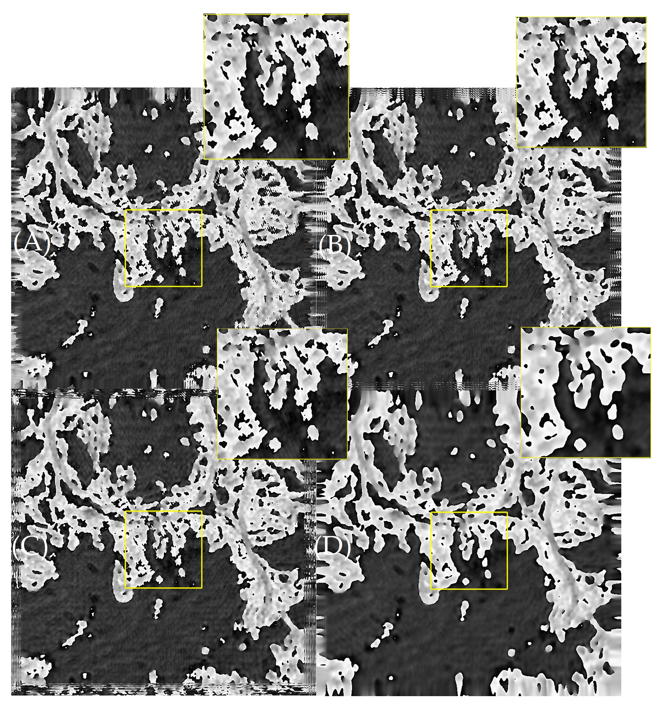
In order to demonstrate the superiority of the D-FFT (Tukey) algorithm for reconstructing the phases in practical applications, the phases reconstructed by different algorithms are shown in Figure 11.

When comparing the phases reconstructed by the four algorithms, as shown in Figure 11, it can be observed that lung cancer cell edges of the phases reconstructed by D-FFT, T-FFT, and D-FFT (rect) are often discontinuous, whereas the phases reconstructed by the D-FFT (Tukey) algorithm have smoother edges. In the background of Figure 11, the other three algorithms show noises similar to parallel pinstripes, while the D-FFT (Tukey) algorithm eliminates these noises while preserving the original phase of the lung cancer cells. That is, the D-FFT (Tukey) algorithm obtains a more accurate and higher-quality reconstructed phase, which is consistent with the simulation results.

4. Conclusions

In summary, a more accurate Fresnel diffraction integration algorithm is urgently needed because both the D-FFT algorithm and the T-FFT algorithm cannot obtain accurate amplitude and phase distributions of the diffracted field when dealing with diffraction problems with diffraction distances exceeding the splitting distance. Based on this need, the D-FFT (Tukey) algorithm has been proposed in this paper.

The D-FFT (Tukey) algorithm filters the transfer function using a Tukey window with adjustable edge smoothing, which eliminates the ringing effect while filtering out the phase distortion part of the transfer function. Since the algorithm filters out the phase-distorted portion of the transfer function directly using the Tukey window, it avoids the error caused by using the fast Fourier transform to compute the transfer function when calculating long-distance diffracted fields and thus improves the resolution of the phase distribution. The improved algorithm is suitable for diffraction problems where the diffraction distance is larger than the splitting distance. In particular, the edge smoothing of the Tukey window used for filtering is affected by β. For any diffraction problem, PSNR and SSIM can be calculated according to the actual parameters to select the optimal solution for β, which makes the D-FFT (Tukey) algorithm generalizable.

The improved algorithm proposed in this paper eliminates the under-sampling effect of the transfer function without causing the ringing effect, and a higher resolution of the phase distribution is obtained. It is expected to be applied in areas such as phase correction, structured illumination digital holographic microscopy, and digital holographic microscopy, which have stringent requirements for the reconstruction amplitude and phase.

References

- Tabata, S.; Arimoto, H.; Watanabe, W. Looking through diffusers by phase correction with lensless digital holography. OSA Contin. 2020, 3, 3536–3543. [Google Scholar] [CrossRef]
- Gao, C.; Wen, Y.; Cheng, H.; Wang, Y. Automatic Phase-Distortion Compensation Algorithm in Digital Holography. Acta Opt. Sin. 2018, 38, 105–111. [Google Scholar]
- Zeng, Y.; Lei, H.; Liu, Y.; Hu, X.; Zhu, R.; Su, K. Compensation of the Phase Aberrations in Digital Holographic Microscopy Based on Reference Lens Method. Acta Opt. Sin. 2018, 47, 222–228. [Google Scholar]
- Li, S.; Ma, J.; Chang, C.; Nie, S.; Feng, S.; Yuan, C. Phase-shifting-free resolution enhancement in digital holographic microscopy under structured illumination. Opt. Express 2018, 26, 23572–23584. [Google Scholar] [CrossRef] [PubMed]
- Lai, X.; Tu, H.; Lin, Y.; Cheng, C. Coded aperture structured illumination digital holographic microscopy for super-resolution imaging. Opt. Lett. 2018, 43, 1143–1146. [Google Scholar] [CrossRef] [PubMed]
- Song, S.; Wan, Y.; Han, Y.; Man, T. Self-Interference Digital Holography with Structured Light Illumination for Tomographic Imaging. Chin. J. Lasers 2019, 46, 0509001. [Google Scholar] [CrossRef]
- Yaghoubi, S.; Hossein, S.; Ebrahimi, S.; Dashtdar, M. Structured illumination in Fresnel biprism-based digital holographic microscopy. Opt. Lasers Eng. 2022, 159, 107215. [Google Scholar] [CrossRef]
- Tao, S.; Kong, M.; Liu, W.; Xu, J.; Cheng, F.; Liu, K.; Yang, Z. Microchannel Detection Based on Dual-Wavelength Image-Plane Digital Holographic Microscopy. Acta Opt. Sin. 2023, 43, 88–95. [Google Scholar]
- Wang, Y.; Guo, S.; Wang, D.; Lin, Q.; Rong, L.; Zhao, J. Resolution enhancement phase-contrast imaging by microspheredigital holography. Opt. Commun. 2016, 366, 81–87. [Google Scholar] [CrossRef]
- Atul, K.; Kumar, A.N. Surface topographic characterization of optical storage devices by Digital Holographic Microscopy. Micron 2023, 170, 103459. [Google Scholar]
- Mas, D.; Garcia, J.; Ferreira, C.; Bernardo, L.M.; Marinho, F. Fast algorithms for free-space diffraction patterns calculation. Opt. Commun. 1999, 164, 4–6. [Google Scholar] [CrossRef]
- Yamaguchi, I.; Matsumura, T.; Kato, J.I. Phase-shifting color digital holography. Opt. Lett. 2002, 27, 1108–1110. [Google Scholar] [CrossRef] [PubMed]
- Desse, J.M. Recent contribution in color interferometry and applications to high-speed flows. Opt. Lasers Eng. 2006, 44, 304–320. [Google Scholar] [CrossRef]
- Li, J.; Tankam, P.; Peng, Z.; Picart, P. Digital holographic reconstruction of large objects using a convolution approach and adjustable magnification. Opt. Lett. 2009, 34, 573–574. [Google Scholar] [CrossRef] [PubMed]
- Li, J.; Peng, Z.; Fu, Y. Diffraction transfer function and its calculation of classic diffraction formula. Opt. Commun. 2007, 280, 243–248. [Google Scholar] [CrossRef]
- Goodman, J.W. Introduction to Fourier Optics, 3rd ed.; Roberts and Company Publishers: Greenwood Village, CO, USA, 2005; pp. 70–71. [Google Scholar]
- Zhang, Y.; Zhao, J.; Fan, Q.; Yang, S. Application of Digital Holography in Phase Measurement. Chin. J. Lasers 2010, 37, 1602–1606. [Google Scholar] [CrossRef]
- Wei, S.; Chen, X.; Wen, Y.; Cheng, H. Research on Edge Error Suppression Method of Reconstructed Image of Digital Holography. Imaging Sci. Photochem. 2021, 39, 166–173. [Google Scholar]
- Zhang, W.; Zhang, H.; Jin, G. Single-Fourier transform based full-bandwidth Fresnel diffraction. J. Opt. 2021, 23, 035604. [Google Scholar] [CrossRef]
- Liu, C.; Wang, D.; Zhang, Y. Comparison and verification of numerical reconstruction methods in digital holography. Opt. Eng. 2009, 48, 105802. [Google Scholar] [CrossRef]
- Kyoji, M.; Tomoyoshi, S. Band-Limited Angular Spectrum Method for Numerical Simulation of Free-Space Propagation in Far and Near Fields. Opt. Express 2009, 17, 19662–19673. [Google Scholar]
- Zhang, W.; Zhang, H.; Jin, G. Band-extended angular spectrum method for accurate diffraction calculation in a wide propa-gation range. Opt. Lett. 2020, 45, 1543–1546. [Google Scholar] [CrossRef] [PubMed]
- Lei, Z.; Fei, W.; Li, Y.; Wang, K.; Bai, J. Semi-analytic Fresnel diffraction calculation with polynomial decomposition. Opt. Lett. 2022, 47, 3776–3779. [Google Scholar]
- Liu, Y.; Sun, Q.; Chen, H.; Jiang, Z. Fractional Fourier-transform filtering and reconstruction in off-axis digital holo-graphic imaging. Opt. Express 2023, 31, 10709–10719. [Google Scholar] [CrossRef] [PubMed]
- Kreis, T. Handbook of Holographic Interferometry: Optical and Digital Methods; John Wiley & Sons: Hoboken, NJ, USA, 2006; pp. 81–183. [Google Scholar]
Figure 1.
(A) Tukey windows for different β values; (B) phase of before improvement; (C) phase of after improvement.
Figure 2.
Intensity profiles through center of Young’s double−hole experimental fringes obtained by (A) D-FFT; (B) T-FFT; (C) D-FFT (rect); and (D) D-FFT (Tukey) ().
Figure 3.
Intensity profiles through center of Young’s double-hole experiment fringes obtained by D-FFT (Tukey): (A) ; (B) ; (C) ; (D) .
Figure 4.
Different algorithms for USAF1951’s reconstruction results of the PSNR curves and SSIM curves: (A) PSNR curves; (B) SSIM curves.
Figure 5.
Intensity and phase of reconstruction images obtained by (A) D-FFT (Tukey) () and (B) T-FFT.
Figure 6.
Profiles of normalized phase obtained by D-FFT (Tukey) () and T-FFT: (A) located in group 7, element 2 (in the blue box in Figure 5); (B) located in the rectangular window of group 7 (in the red box in Figure 5).
Figure 7.
Light path diagram of holographic microscopy experiment on lung cancer cells.
Figure 8.
Different algorithms for lung cancer slice’s reconstruction results of the PSNR curves and SSIM curves: (A) PSNR curves; (B) SSIM curves.
Figure 9.
Intensity of reconstruction images obtained by different algorithms: (A) D-FFT; (B) D-FFT (rect); (C) T-FFT; (D) Tukey ().
Figure 10.
Profiles of reconstructed intensity obtained by different algorithms: (A) intensity profile plots (dashed line in yellow box); (B) intensity profile plots (solid line in red box).
Figure 11.
Phases reconstructed by (A) D-FFT; (B) D-FFT (rect); (C) T-FFT; and (D) D-FFT (Tukey) ().