1. Introduction
Ground-penetrating radar (GPR) uses electromagnetic pulses to explore beneath the earth’s surface, a crucial process for assessing soil layers and infrastructure in the railroad sector. GPR systems consist of an emitting antenna and a receiving unit for reflected signals. The signal data are processed into an image, known as radargram, which reveals subsurface features. In railroad applications, the primary use of GPR is to ascertain the thickness and composition of soil layers along railroad tracks [
1,
2]. This information is critical to planning and executing maintenance activities on railroad infrastructure. Additionally, GPR plays a key role in underground object detection, including the identification of explosive ordnances beneath railroad tracks. This capability enables early hazard detection and facilitates prompt response measures.
Despite its extensive utility, the application of object detection in GPR is not without challenges. Existing learning algorithms for object detection, which have seen success in various domains, rely heavily on manually labeled data from real measurements [
3,
4,
5]. This approach necessitates prior knowledge of the subsurface, a requirement often unmet in the context of object detection beneath railway tracks. While some data for soil layer analysis might be partially labeled, providing ground truth, the same is not true for object detection. The manual labeling of such data would be labor-intensive and impractical, as verification would require extensive excavation.
To address these challenges, an innovative approach that does not rely on manually labeled data is proposed in this work, where physics-based simulation data are leveraged to fill this gap. Simulated data have already been used in the verification of processing pipelines, for example, in the detection of objects in tunnel linings [
5], but models applied to real data require training on labeled real-world samples. While the effectiveness of enhancing detection models with simulated data has also been previously established [
6], manual efforts are rendered completely unnecessary in this approach. Even though success has been shown by non-physics-based methods, particularly those employing Generative Adversarial Networks (GANs), for tasks like radargram de-noising [
7], they have largely been confined to two-dimensional applications [
8,
9]. The rich information available in multi-antenna GPR systems, particularly vital to detecting objects where significant signal variations across channels are observed, is neglected by such methods. The aim of this paper is to harness such additional channel information to enhance object detection models in railroad track beds. The generation of high-quality training data also requires substantial fine tuning to achieve optimal results. Additionally, this work aims at developing a fully automated process pipeline that operates without any manual intervention, thereby greatly simplifying future developments in object detection algorithms for railway applications.
The initial phase involves simulating data from a multi-antenna GPR system by using the specially developed digital twin of a GPR antenna. This simulation aims to produce data that closely mirror real-world scenarios. Subsequently, a learning algorithm is applied to this simulated dataset to develop predictive models for object detection in radargrams. The final phase of this work entails applying these models to actual data, using a controlled environment where specific objects are buried along a known route. This approach allows for detailed analysis and comparison of the models and the assessment of their performance and transferability in multi-antenna radargram object detection.
Ground-Penetrating Radar
Ground-penetrating radar emits electromagnetic waves into the ground, as illustrated in
Figure 1; waves are partially transmitted and reflected at boundaries with different electromagnetic properties, and reflections are captured by a receiving antenna to infer ground composition [
10]. Individual GPR signals, known as A-Scans, are typically compiled into two-dimensional representations for analysis. These are designated as B-Scans (radargram, YZ-plane), C-Scans (XY-plane), or D-Scans (XZ-plane), depending on their plane orientation (see
Figure 1d).
The propagation speed of an electromagnetic wave
v in a medium can be approximated from the ratio of the speed of light in vacuum (
) and the square root of the product of relative permeability (
) and relative permittivity (
) ([
11], p. 149):
Moving an antenna over a reflective object thus alters the signal’s travel time, creating hyperbolas in B- and C-Scans due to changing distances.
2. Materials and Methods
Figure 2 delineates the architecture of the developed methodology, with each segment receiving a detailed exposition in the subsequent chapters of this document. Initially, a digital twin representation is created and utilized within the track simulator to generate synthetic data, as detailed in
Section 2.2 and
Section 2.3, respectively. These synthetic data, alongside empirical data collated from a reference track, detailed in
Section 2.5, are both subjected to a unified process of pre-processing and channel reduction, described in
Section 2.4 and
Section 2.7. The refined artificial data from this process are instrumental in the training of an object detection model, elaborated in
Section 3.3, which is integral to the subsequent detection routine, explored in
Section 2.9.
2.1. Simulation Framework
In the course of this project, the simulation software “gprMax”, version 3.1.6, available at the time of this work, was used [
12]. This software is an open-source project specifically developed for the modeling of ground-penetrating radar systems and similar applications, and it is widely used in this field for the simulation of GPR systems.
2.2. Digital Twin of GPR Antenna
Due to technical limitations, achieving a perfect match between computer-generated data and real system data is fundamentally impossible, leading to a discrepancy referred to as domain gap, which poses a significant challenge in the use of computer-generated data for training learning algorithms. In this work, the AM200 antenna system by IDS GeoRadar s.r.l. (Pisa, Italy) was utilized, and to enhance the transferability between these domains, a digital twin of the system was developed. This development employed Taguchi optimization, a methodology documented by Warren and Giannopoulos [
13].
Initially, the gprMax simulation environment was used to generically replicate the core components of the antenna and the experimental setups, with the determination of their properties being the subsequent step. Reference measurements were then conducted by using the selected GPR system, focusing on measuring the antenna crosstalk and the reflection on a metal sheet. The measurement of antenna crosstalk, which is the signal that travels directly from the transmitting antenna to the receiving one, was carried out in a dedicated antenna laboratory to minimize interference, as illustrated in
Figure 3a. The choice of metal sheet reflection as a measurement parameter was due to its high replicability in the simulation environment and the setup for measurement, which is depicted in
Figure 3b.
Through the application of an iterative optimization algorithm, an optimal combination of parameters was established. Consequently, the developed model not only captures the geometric details of the antenna system but also incorporates its essential physical properties, which is crucial to simulating electromagnetic wave propagation. While the information obtained may not cover the entire complexity of the antenna system, comparative measurements, as depicted in
Figure 4, demonstrate a close correspondence between the actual antenna used and its digital twin.
2.3. Track Simulator
The basis for simulating a railway track is gprMax software, which simulates the propagation of electromagnetic waves in a defined environment. However, it became apparent during the work that the basic functionalities were not sufficient to fully meet the requirements. Building on the functions of gprMax, software tailored to the simulation of railway tracks was developed, meeting the needs of this work. The software is explained as follows.
2.3.1. Construction of Railway Track
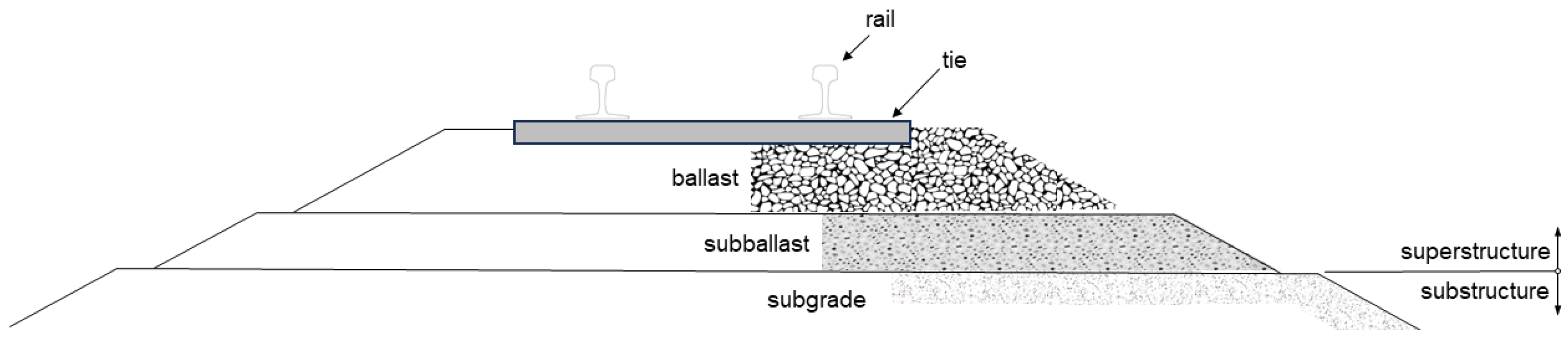
The substructure of a railway track is generally divided into several layers [
14], as illustrated in
Figure 5. The top layer consists of coarse-grained ballast, in which the sleepers are embedded. Beneath it is the subballast layer, which serves as a separating layer to prevent the mixing of the ballast bed with the bottom layer, the subgrade, and provides drainage. This layered structure was used as a basis for the simulation and replicated in the simulation environment, with the resulting simulation environment being depicted in
Figure 6. It is noted that the ballast was modeled separately, where each individual ballast grain was generated randomly and piled up through physics-based simulation. Additionally, the subgrade layer consisted of a soil model with varying degrees of moisture, thus replicating diverse subballast conditions.
2.3.2. Simulation Space
Due to gprMax’s calculation method, where the entire simulation space is divided into equally sized cells, the computational effort and memory consumption increase to the third power with the enlargement of the simulation space. This creates a limit on the maximum possible simulated space, mainly determined by the memory capacity of the hardware used. For this work, a server consisting of eight NVIDIA RTX™ A6000 graphics processors, each with 48 GB of memory, was used. With a resolution of 2 mm, this allowed for a maximum simulation space of up to approximately 1.6 m × 1.5 m × 1.6 m. Additionally, the simulated space can be restricted in the direction of travel to the extent that a clean formation of hyperbolas resulting from reflection on objects is achieved. In this case, this was achieved with a simulated distance of 1 m, resulting in a minimal simulation space per section of 1.6 m × 1.0 m × 1.6 m.
Extended tracks were simulated within this constraint by initially segmenting each track into smaller parts, which were then individually simulated on separate graphics processors. The individual results were then reassembled. The requirement to traverse the entire track in sections necessitates a programmatic method for creating individual segments in the simulation environment. For this purpose, an automatic generation routine was developed. Based on a general configuration file, outlined in
Section 2.3.3, individual gprMax simulation environments were defined, as detailed in
Section 2.3.4, resulting in simulation segments, as depicted in
Figure 6.
2.3.3. Configuration
The configuration file for the track simulator contained information about the entire track, including the geometry of the soil layers, the position of objects, and their material properties. It also included the general parameters of the track, which were fixed for the easier further processing of the data. These included the simulated space, spatial resolution, and maximum simulation time. The maximum sensible simulation time results from the signal transit time of the excitation pulse. Assuming an average permittivity of
, a depth of 1.6 m requires at least a transit time of the forward and return wave of approximately 34 ns (see Equation (
1)). To enable a good comparison with real data, a simulation duration of 40 ns was chosen. Additionally, the antenna polarization, which determines the direction of the emitted fields based on the type and installation position of individual antennas, can be set. In this work, VV polarization was chosen (Vertical–Vertical), where both the transmitting and receiving antennas are arranged parallel to the direction of movement.
2.3.4. Automated Scenario Generation
Text files (input files) are used as an interface in gprMax simulation software, containing all information for conducting a single simulation. Various commands are available to define objects (geometry, position, etc.), material properties (permittivity, conductivity, etc.), or general properties (simulation time, resolution, etc.). These commands are each marked by a hash symbol (#) in the text file.
The task of the generation script is the automated creation of the input files, based on the defined track in the configuration file (see
Section 2.3.3). This process involves extracting specific information for each segment based on its position from the configuration file and translating this information into gprMax commands. By creating separate input files for each segment, the generation script enables the modular and efficient execution of simulations. Each segment can be simulated independently, improving the parallelization and scalability of the simulations. Additionally, managing separate text files for track segments facilitates the post-processing and analysis of simulation results for individual sections of the track.
Beyond the standard track and sleepers in each section, the substructure can incorporate extra objects with customizable material properties. Not being limited to basic shapes like cuboids, cylinders, and spheres, it also supports the integration of digital design files, regardless of size and complexity. The antennas were based on the digital twin of a ground-penetrating radar system, as described in
Section 2.2. They were inserted in triplicate in the middle in the direction of travel and a defined transverse offset, so as depicted in
Figure 7, a total number of 11 channels were available for evaluation by default.
The output of a simulation run is structured as a folder structure. In addition to the measurement results, which are available channel-wise for each track segment as .out files, additional data from the simulation environment (resolution, objects, substructure course, etc.) are stored as .json files. To enable a meaningful further processing of the simulation data, each channel is accompanied by a Label.txt file, which defines the positions of the objects visible in the respective channel.
2.3.5. Simulation Time
A crucial aspect of the developed track simulator is the calculation time required per track section, which is significantly dependent on the simulation parameters used.
Table 1 lists those parameters that are expected to have a direct influence on the required computation time, along with the respective influence factor. A runtime factor of
is to be interpreted as a purely linear change in simulation duration caused by a change in the parameter. However, the factor
already implies an increase in the required computation time to the third power with a linear change in the parameter.
In absolute numbers, this results in an average simulation duration of 154 min per simulated meter of track section for the final parameter combination used in this work. Even though decreasing the step size from 2 cm to 4 cm results in the simulation time dropping to 77 min, and a further halving of the spatial resolution cuts down the simulation time by approximately 87.5%, the decision was made not to reduce it in order to ensure high quality of the simulation results.
2.4. Pre-Processing
To efficiently utilize data obtained from a ground-penetrating radar, they are typically processed through a series of post-processing steps. The antenna model underlying this work is based on the previously developed digital twin of a real antenna. Consequently, the simulation results based on this model closely match those of the real antenna, allowing for the application of the same post-processing steps. These steps are illustrated in
Figure 8 and documented below in the order of their application.
2.4.1. Removing Signal Anomalies
In the context of this research, neither the simulated nor the real datasets exhibited relevant noise. However, a drift along the time axis was detected in both. This temporal drift was attenuated through the application of a moving average filter, utilizing a temporal window of 2.5 ns.
2.4.2. Downsampling
The simulated data were calculated at a higher temporal resolution than that for the real data. To avoid unnecessary computational effort, all data were reduced to 5 samples per nanosecond.
2.4.3. High-Pass Filter along Time Axis
To remove potential drift in the signal, a sliding average was subtracted, with the window width set to 2.5 ns. Although almost no drift was noticeable in the simulated signals, the same filtering process as for the real data was applied for the reasons mentioned above.
2.4.4. Adjusting of Measurement Window
In the real system, a slightly delayed recording start of the cross-antenna channels (No. 4 and 5) was observed. To compensate for this delay, the mentioned channels were shifted accordingly. The iteration at which a channel first reached a spike of 10% of its maximum value served as the new zero position. To improve the processing of real and simulated measurement results, all measurements were additionally reduced to a uniform length of 40 ns.
2.4.5. Dewow Filter
The so-called “wow” of the signal is a slow, wave-like signal component along the path axis of a recording which can arise, for example, from the inductive coupling of the antenna with the earth’s surface [
15]. To remove these low-frequency signal components (dewow) along the path axis, a sliding average filter was also used. The filter length was chosen such that larger structures, which could originate from buried objects, would remain visible.
In this work, predominantly short track sections of a few meters were created, where a “wow” in the above sense generally does not pose a problem. However, low-frequency signal components along the path axis did occur in the form of antenna crosstalk.
Figure 9a,b first show an unprocessed B-scan and then the result after applying the dewow filter. While the unprocessed B-scan (see
Figure 9a) is dominated by antenna crosstalk, the latter is completely removed in the filtered B-scan (see
Figure 9b).
2.4.6. Absorption Compensation
Deeper objects increasingly disappear into the background due to the quadratic power decrease in the electromagnetic wave during propagation and the additional attenuation through the material to be penetrated. Despite the existence of more sophisticated methods, like spectral balancing [
16], a simple empirically derived gain function was chosen to mitigate this effect. This function dampens early signals and progressively boosts the signal strength further along the time axis. However, the noise components of the signal are also amplified by the increasing amplification, as evidenced by the results shown in
Figure 9c.
2.5. Reference Track
To assess the quality of the simulated data and to evaluate the performance of the subsequently developed detection algorithm, real measurement data from a known track were used. This enabled the validation of the simulated data, ensuring that the simulation models adequately reflected actual conditions. The following subsections address the specifics of the track and the measurement process.
2.5.1. Real-World Measurement
The measurement was conducted on a railway siding using a GPR antenna of type AM200 from the manufacturer IDS GeoRadar s.r.l., Pisa, Italy. This antenna was mounted 8 cm above the sleepers on a measuring cart and moved evenly along a track distance of 51 m. Individual measurements were triggered every 2 cm by using a distance-measuring wheel. Various objects were buried at defined distances along the track, as listed in
Table 2. In addition, there were concrete sleepers spaced 65 cm apart on the track extending across the entire measurement area. To facilitate a good comparison between the reference track and the simulated data, both the real and simulated data were processed by using the same methods described in
Section 2.4.
2.5.2. Comparison of Measurement Data
Figure 10 and
Figure 11 show the complete B-scan of the middle channel (No. 4) for both real and simulated data. To better illustrate this, the areas where objects were buried in the B-scan of the real measurement are marked in red. In comparing real and simulated measurements, the first key observation is the presence of consistent reflections from the upper area’s sleepers. Similar reflections further down indicate transitions between the ballast layer, subballast, or subgrade due to varying materials. Expectedly, these transitions show gradually changing reflection heights. However, the upper sleeper contours are echoed in lower layers, with high-frequency waviness along the path axis due to electromagnetic wave traversal. In the simulated data, the absence of low-frequency components is noted due to constant subgrade layer thickness, unlike the real dataset, where gradual subgrade changes are observed over long track segments. Distinct variations are evident in the real data for buried objects beneath the track. Metal containers at 10 m and 50 m are distinctly visible, exhibiting hyperbolas of differing prominence, most probably attributed to variations in their depths and orientations. In simulations, these containers also exhibit clear hyperbolas. The water container at 19.7 m, while similar to the metal containers, shows unique multiple reflections for differentiation, a feature well represented in simulations. Distinguishing between the buried log and rock at 30 m and 40 m is challenging. While the relative permittivity of wood is about
to
, slightly lower than that of granite (
), the permittivity of the rock can be assumed to be similar to that of granite. The slight difference in permittivity between wood and granite-like rock did not produce clear reflections in either real or simulated data. However, a certain irregularity in the signal is noticeable at both positions (30 m and 40 m) directly below the sleepers. Regardless of whether these changes were due to the objects or whether the excavation work carried out at these points itself affected the measurement, these positions served as control points. They allowed for the verification of whether the subsequently implemented algorithms actually responded to the sought-after objects or were equally sensitive to general structural changes beneath the track.
2.6. Detection Framework
In traditional object detection approaches, a sliding window is either moved across the input image or the image is divided into various regions, each requiring a computation cycle, thereby increasing the computational effort needed per image. The You Only Look Once (YOLO) framework [
17], acting as a single-shot detector, was utilized in this study, enabling the identification of all detected objects in the input image through just one model evaluation. This efficiency is achieved by consolidating all detection steps into a single model. The choice of this framework was influenced by its suitability for processing live data in future applications. By enabling image processing through a single evaluation, the YOLO framework significantly lowers computational demands, making it highly suitable for tasks involving real-time object detection.
2.7. Channel Reduction
The YOLO detection framework is originally designed to handle three-dimensional data, typically limited to the Red, Green, and Blue (RGB) color channels.
Two main strategies were employed to adapt the ground radar dataset, comprising 11 channels along with time and path axes, to the three-channel format: data subset selection and dimensionality reduction through feature selection. Both strategies were explored in the work of this study, resulting in varying outcomes. Inspired by the method of Kim et al. [
3], the subset selection approach entailed the creation of three cross-sectional views for each subsection, with one view being assigned to each RGB channel. However, satisfactory results were not yielded by this method; thus, it is not elaborated upon in this paper. The approach found to be more effective, which is detailed further, revolves around the engineering of lower-dimensional features to effectively condense the data into a format compatible with the YOLO framework.
2.7.1. Data Mapping Analogous to LiDAR Sensor Processing
Drawing on the “bird’s eye” perspective utilized in LiDAR sensor (Light Detection and Ranging) data analysis, this paper proposes a comparable approach for analyzing simulated georadar data. LiDAR sensors provide a three-dimensional point cloud of the environment and are used, for example, in the localization of autonomous robots and the detection of their surroundings. Due to the operation, where a rotating laser outputs the current angle and the measured distance, a point cloud consisting of the nearest reflective surfaces around the sensor is created [
18]. The vertical resolution is usually very limited compared with the angle resolution, but here too, the need arises to reduce the horizontal levels. In the case of point clouds, this is performed by encoding the three-dimensional dataset onto three horizontal image planes. The first image plane describes the height of the highest reflected point at each position, while the second plane records its intensity. The total number of reflected points at each position is entered on the third plane [
19]. Unlike LiDAR data, where few points are occupied in the entire space, ground radar measurement data have an intensity value for every point, making a simple transfer of the aforementioned encoding impractical. The following are various processing methods aimed at highlighting the characteristic properties of ground radar data.
2.7.2. Average of B-Scans
By forming the average in the channel direction, signal components that extend over all channels are amplified. In contrast, reflections visible in only a few channels are weakened. As a result, sleepers, which extend over the entire measurement area and beyond, are especially well represented (see
Figure 12a).
2.7.3. Standard Deviation in Channel Direction
A measure of the change in signal strength is the standard deviation (
), which is calculated by using the mean value (
) and the number of channels (
n) as follows:
Applied to each data point across the individual channels, differences between the channels are emphasized. This particularly highlights reflections in the subgrade, which only occur in individual channels, such as smaller objects in the ground radar’s measurement range (see
Figure 12b).
2.7.4. Normalized Deviation
The normalized deviation (
z) has proven to be more robust than the simple standard deviation, which is also applied across all channels. Each value (
x) is reduced by the respective mean value (
) between the channels and then normalized by the standard deviation (
) of the values between the channels [
20]:
The result, shown in
Figure 12c, clearly shows the difference from simple standard deviation.
2.8. Data Augmentation
Given the significant computational resources required to create individual data samples, the resulting dataset was relatively small. To enhance the training foundation, data augmentation presents a viable solution. The augmentation techniques focused on the following dataset properties:
Mirroring;
Scaling;
Resolution;
Noise level.
These data augmentation methods were carefully chosen to reflect realistic conditions of objects buried underground. Objects can vary in size and orientation, warranting the adoption of scaling and mirroring techniques. Moreover, because the resolution and noise levels do not perfectly align with the real system, even when using a digital twin, employing augmentation methods for resolution and noise level proves practical.
The mirroring of the data was performed both horizontally and vertically, with the data along the path axis being additionally stretched or compressed by %. Both for time (vertical axis) and path (horizontal axis), the resolution was reduced by up to 50%. The added noise was normally distributed and was chosen so that the average signal-to-noise ratio across the entire dataset was at least 25 dB.
2.9. Implementation of the Automatic Detection Routine
The reference track, with a length of 51 m, differed significantly from the simulated meter-long sections used for training. To apply the trained model to the reference track, it had to be broken down to the same size and was thus divided into 1 m pieces. To prevent the incorrect detection of objects in the border areas, an overlap of 0.5 m was chosen for successive pieces. The detection algorithm proceeds as follows: After initialization and algorithm instantiation from the configuration file, measurement data are read, pre-processed, and fed to the algorithm. The trained model is loaded, and a process pool is created for converting data into the dataset, as described in
Section 2.7. The data are segmented, processed, and analyzed by the model. The computation results are normalized to the track’s original length. Overlapping detections are refined, keeping only the most probable ones and filtering out low-probability detections. These results are then compared with the reference track’s ground truth. The labels of detections are overlaid with the ground truth, calculating precision and recall based on their intersection over union (IoU). Finally, the outcomes are exported as text files and files in Visualization Toolkit (VTK) format, which are suitable for three-dimensional visualization.
3. Results
Initially, the generated simulations are analyzed and compared to actual data to identify any discrepancies. Following this, the outcomes of the algorithms developed are reviewed.
3.1. Simulations
Over the course of the work, more than 700 individual simulations were used to replicate over 50 different track environments under various conditions.
Figure 13 compares the B-scan of a section from the real dataset with the corresponding simulation result. Visible in this section are three sleepers (narrow hyperbolas in the upper area) and a buried metal container, which appears as a hyperbola between the second and third sleepers.
A mere examination of the B-scans already reveals a high degree of similarity, although the sleepers in the simulated data appear somewhat clearer. This can be attributed to slight differences in the assumed and actual material properties. When comparing the normalized deviation, shown in
Figure 14b, the reflection components of the sleepers are also overemphasized. This effect suggests a deviation of the antenna model from the real antenna.
In the examination of the C-scan at the sleeper level (see
Figure 15), it is evident that channels 4 and 8 are attenuated in the simulated data. These channels are those cross-track channels where the transmitting and receiving antennas are located in different housings. Even though this configuration was not explicitly replicated during the development of the digital twin and thus slight deviations from the real setup have to be expected, the effect is observed in both the real and simulated data.
Traditional similarity criteria, such as the mean square deviation, are unsuitable in this case, as the absolute position of the objects significantly influences the result. However, this is of secondary importance for the present problem.
A more suitable method for evaluating similarity is the structural similarity (SSIM) described by Wang et al. [
21], which is widely used in image processing. In addition to contrast and brightness, the structure of the image is also evaluated. For each image area, a normalized value between −1 and 1 is determined, with a value of 0 indicating no similarity and +1 absolute equality. A value of −1 would correspond to the inverted image. Applied to the results in
Figure 13, this yields an average SSIM value of 0.95, indicating a high degree of similarity. When only the image section in the area of the sleepers and the buried object is considered, the average SSIM value is slightly lower, 0.84, but also confirms very high similarity here. Applied to the normalized deviation, visible in
Figure 14, SSIM values of 0.95 for the entire image or, likewise, 0.84 for the relevant section are obtained.
3.2. Preparation and Composition of Dataset
All data underwent pre-processing to be properly formatted for the neural network training of YOLO. For the scope of this work, the dataset was limited to 20 simulated track sections of 1
each. Future investigations, however, can use the present research as a basis and expand the dataset analogously. This led to the decision to initially distinguish between only two classes: the railroad sleepers and the buried containers.
Figure 16 shows a dataset that was reduced to three channels by using the approach described in this paper. To expand the overall dataset, the methods of data augmentation described in
Section 2.8 were relied upon. This resulted in a dataset of 56 sleepers and 40 metal containers underground which was used for training.
3.3. Training of Object Detection Model
The image size for training was set to 1280 px and the number of training iterations to 300 px. The number of images combined per training iteration (batch size) was 8. In addition to the augmentation methods listed above, additional integrated methods in the framework were applied to all data. These were defined via a configuration file and included, among others, the following:
In mosaic arrangement, several training images are randomly combined into a single image, which may lead to overlaps between the original images and possibly the concealment of individual labels. This approach offers the advantage that a model trained with such data is better able to recognize objects at positions where no objects were present in the training dataset.
The basis for the transformation of color information is the Hue, Saturation, and Value (HSV) color model, which describes the hue, saturation, and brightness of an image. However, it must be noted in the present case that fundamentally different information is applied to the individual color channels of the image, which makes, for example, a change in hue impractical.
The box loss serves as a metric for training. Both for the training and validation datasets, a significant decrease in errors with the increase in training progress was observed, suggesting advantageous development of the model.
3.4. Evaluation
Upon examination of the data presented in
Figure 17, the model, which was trained by utilizing the artificial dataset, demonstrated notably high efficacy in the detection of individual sleepers. This robust detection was characterized by consistent and precise recognition across the entire length of the track.
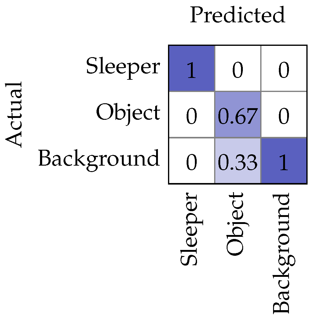
This is also evident when looking at the confusion matrix (see
Figure 18), which shows a 100% recognition rate. While the precision for buried objects is also 100%, the recall rate is only 66%. However, due to the uneven distribution of classes, the resulting average precision of 83% is of limited significance. Some variability is also evident in the dimensions and positions of the labels, reflected in an average IoU value of 61% for sleepers.
3.4.1. Object Detection Computation Time
The total computation time for the 51-m-long reference track, encompassing a total volume of 14.37 million voxels, amounted to . Of this, roughly 90% ( ) was dedicated to data pre-processing, leaving for the actual inference process.
3.4.2. Degree of Automation in Process Chain
The entire process, from preparing the simulation data and generating labels to detecting objects on a given track, is fully automated. Manual user input is only necessary when defining the track sections to be simulated and possibly when tuning the parameters of the YOLO framework. A critical point in this process chain is the correct placement of labels, as this is crucial to the proper functioning of the resulting model. The proposed method was found to be robust in this respect due to the chosen calculation methods.
4. Discussion
The challenge in developing algorithms using artificial intelligence often lies in providing high-quality datasets. Particularly, in detecting objects buried in railway beds, the available datasets are not sufficient in either quality or quantity. This is partly due to the fact that the verification of manually labeled data would require extensive excavation work, which seems highly impractical given the necessary volume of data. The primary aim of this project is to create an automated process for generating physically accurate data, labeling them, and subsequently applying algorithms that have been trained on this dataset on real-world environments.
To achieve the objective, a digital twin simulating the electromagnetic properties of a real GPR antenna system was developed and integrated into a simulation environment tailored for the railway sector. This allows for the simulation of measurements in customizable railway scenarios, providing realistic data and ensuring that ground truth is available for subsequent training steps. The processing of simulated radar data was undertaken by using two distinct methods, with a focus on the additional insights gained from utilizing all channels of a multi-antenna system. These data were transformed into RGB images, where each color channel conveyed different information, enabling direct training with the YOLO framework. The detection model was demonstrated to be capable of identifying objects within the railway bed by using exclusively synthetic training data. The performance of the model and its transferability to real-world data were evaluated through measurements on a reference track, where known objects had been buried in advance. These measurements were then compared with the predictions of the model to assess accuracy and reliability.
This work represents a significant advance in the application of artificial intelligence in the railway sector by overcoming the challenge of high-quality training data scarcity through the use of realistic simulation models by leveraging the digital twin of an multi-antenna system. The created simulation environment effectively generates realistic GPR measurements for various railway environments and subsoil conditions, avoiding the need for the costly gathering of labeled real-world data. This advancement not only simplifies future research in object detection and beyond but also introduces a novel method for transferring the three-dimensional radar data of a multi-antenna system, enabling the efficient use of all system channels within established detection frameworks, marking a novel application in the railway industry.
Although the feasibility of developing detection algorithms exclusively with artificial data has been demonstrated, the limitations of this approach must be acknowledged. Firstly, the results might not be universally applicable to other antennas due to the customization of the digital twin to a specific antenna. Additionally, a risk of overfitting was indicated by the restricted dataset used in this study, suggesting that an expansion of the dataset should be aimed for in future research to enhance reliability. It is also acknowledged that the performance of various detection frameworks may vary, with some potentially outperforming the chosen YOLO framework. Therefore, identifying the most suitable detection framework necessitates comparative testing. Moreover, the applicability of the chosen processing methods to objects with varying radar-reflection characteristics remains uncertain. While the differentiation between two types of objects (sleepers and buried containers) has been successfully achieved, the efficacy in distinguishing among various buried objects, such as metal containers and water-filled boxes, has yet to be tested. Lastly, the basis for the evaluation of model performance has been a singular reference measurement, which may not accurately reflect the breadth of potential application contexts. As a result, the need arises to further study the effectiveness of the model across different environments.
5. Conclusions and Outlook
One possible improvement to the existing approach would be to reduce the spatial resolution; this, however, would require a revision of the digital twin. The simulation duration achieved in this work could be further reduced, but the resulting effects on the quality of the measurement data must be carefully examined.
In summary, this work offers a promising approach to improving object detection in the railway sector through the use of a specially adapted simulation environment (gprMax). Despite the identified limitations, there is great potential for further applications and development. This work opens up the possibility of detecting a wide range of buried objects and differentiating between different types of objects while eliminating the need for extensive manual data preparation in the future. By enhancing the simulation environment’s capabilities to model scenarios like ballast contamination or water anomalies, significant potential exists for further refining the ability to simulate various subsoil conditions. This opens up opportunities for developing and testing algorithms aimed at assessing the railway bed or verifying assumptions about its condition, all while minimizing the need for extensive labeling tasks. Consequently, this work provides a solid foundation for further developing methods of all kinds based on the use of ground-penetrating radar systems in the railway sector.
Author Contributions
Conceptualization, L.L. and D.G.; methodology, L.L.; software, L.L.; investigation, L.L. and D.G.; resources, M.B. and G.Z.; data curation, L.L.; writing—original draft preparation, L.L.; writing—review and editing, L.L. and G.Z.; visualization, L.L.; supervision, G.Z.; project administration, D.G. and M.B. All authors have read and agreed to the published version of the manuscript.
Funding
This research was funded by Plasser & Theurer, Export von Bahnbaumaschinen, Gesellschaft m.b.H.
Institutional Review Board Statement
Not applicable.
Informed Consent Statement
Not applicable.
Data Availability Statement
The datasets presented in this article are not readily available because confidentiality reasons. Requests to access the datasets should be directed to Lukas Lahnsteiner.
Conflicts of Interest
Authors Lukas Lahnsteiner, David Größbacher and Martin Bürger were employed by the company Plasser & Theurer. The remaining author declares that the research was conducted in the absence of any commercial or financial relationships that could be construed as a potential conflict of interest. The funder was not involved in the study design, collection, analysis, interpretation of data, the writing of this article or the decision to submit it for publication.
References
- Olhoeft, G.; Smith, S.; Hyslip, J.; Selig, E. GPR in railroad investigations. In Proceedings of the Tenth International Conference Ground Penetrating Radar, Delft, The Netherlands, 21–24 June 2004; Volume 2, pp. 635–638. [Google Scholar] [CrossRef]
- Benedetto, A.; Tosti, F.; Bianchini Ciampoli, L.; Calvi, A.; Brancadoro, M.G.; Alani, A.M. Railway ballast condition assessment using ground-penetrating radar—An experimental, numerical simulation and modelling development. Constr. Build. Mater. 2017, 140, 508–520. [Google Scholar] [CrossRef]
- Kim, N.; Kim, S.; An, Y.K.; Lee, J.J. Triplanar Imaging of 3-D GPR Data for Deep-Learning-Based Underground Object Detection. IEEE J. Sel. Top. Appl. Earth Obs. Remote Sens. 2019, 12, 4446–4456. [Google Scholar] [CrossRef]
- Li, H.; Li, N.; Wu, R.; Wang, H.; Gui, Z.; Song, D. GPR-RCNN: An Algorithm of Subsurface Defect Detection for Airport Runway Based on GPR. IEEE Robot. Autom. Lett. 2021, 6, 3001–3008. [Google Scholar] [CrossRef]
- Qin, H.; Zhang, D.; Tang, Y.; Wang, Y. Automatic recognition of tunnel lining elements from GPR images using deep convolutional networks with data augmentation. Autom. Constr. 2021, 130, 103830. [Google Scholar] [CrossRef]
- Liu, Z.; Gu, X.; Wu, W.; Zou, X.; Dong, Q.; Wang, L. GPR-based detection of internal cracks in asphalt pavement: A combination method of DeepAugment data and object detection. Measurement 2022, 197, 111281. [Google Scholar] [CrossRef]
- Luo, J.; Lei, W.; Hou, F.; Wang, C.; Ren, Q.; Zhang, S.; Luo, S.; Wang, Y.; Xu, L. GPR B-Scan Image Denoising via Multi-Scale Convolutional Autoencoder with Data Augmentation. Electronics 2021, 10, 1269. [Google Scholar] [CrossRef]
- Yue, Y.; Liu, H.; Meng, X.; Li, Y.; Du, Y. Generation of High-Precision Ground Penetrating Radar Images Using Improved Least Square Generative Adversarial Networks. Remote Sens. 2021, 13, 4590. [Google Scholar] [CrossRef]
- Rice, W. Applying Generative Adversarial Networks to Intelligent Subsurface Imaging and Identification. Master’s Thesis, University of Tennessee at Chattanooga, Chattanooga, TN, USA, 2019. Available online: https://scholar.utc.edu/theses/595 (accessed on 14 April 2024).
- Jol, H.M. Preface. In Ground Penetrating Radar Theory and Applications; Jol, H.M., Ed.; Elsevier: Amsterdam, The Netherlands, 2009; p. 4. [Google Scholar] [CrossRef]
- Kark, K.W. Antennen und Strahlungsfelder: Elektromagnetische Wellen auf Leitungen, im Freiraum und ihre Abstrahlung; Springer Fachmedien: Wiesbaden, Germany, 2014. [Google Scholar] [CrossRef]
- Warren, C.; Giannopoulos, A.; Giannakis, I. gprMax: Open Source Software to Simulate Electromagnetic Wave Propagation for Ground Penetrating Radar. Comput. Phys. Commun. 2016, 209, 163–170. [Google Scholar] [CrossRef]
- Warren, C.; Giannopoulos, A. Creating finite-difference time-domain models of commercial ground-penetrating radar antennas using Taguchi’s optimization method. Geophysics 2011, 76, G37–G47. [Google Scholar] [CrossRef]
- Li, D.; Hyslip, J.; Sussmann, T.; Chrismer, S. Railway Geotechnics; CRC Press: Boca Raton, FL, USA, 2015; pp. 72, 104, 108. [Google Scholar] [CrossRef]
- Jol, H. Ground Penetrating Radar: Theory and Applications; Elsevier: Amsterdam, The Netherlands, 2009; p. 34. [Google Scholar] [CrossRef]
- Xavier Neto, P.; Medeiros, W. A practical approach to correct attenuation effects in GPR data. J. Appl. Geophys. 2006, 59, 140–151. [Google Scholar] [CrossRef]
- Redmon, J.; Divvala, S.; Girshick, R.; Farhadi, A. You Only Look Once: Unified, Real-Time Object Detection. arXiv 2016, arXiv:1506.02640. [Google Scholar]
- What Is Lidar? Learn How Lidar Works. Available online: https://velodynelidar.com/what-is-lidar/ (accessed on 17 January 2024).
- Ayyadevara, V.K.; Reddy, Y. Modern Computer Vision with PyTorch: Explore Deep Learning Concepts and Implement over 50 Real-World Image Applications; Packt Publishing Ltd.: Birmingham, UK, 2020; ISBN 978-1-839-21653-4. [Google Scholar]
- Kreyszig, E. Advanced Engineering Mathematics, 10th ed.; John Wiley & Sons, Inc.: Hoboken, NJ, USA, 2011; ISBN 978-0-470-45836-5. [Google Scholar]
- Wang, Z.; Bovik, A.; Sheikh, H.; Simoncelli, E. Image Quality Assessment: From Error Visibility to Structural Similarity. IEEE Trans. Image Process. 2004, 13, 600–612. [Google Scholar] [CrossRef] [PubMed]
Figure 1.
Working principle of ground-penetrating radar (GPR): Electromagnetic waves are partially transmitted and reflected at layer boundaries (a). Multiple individual measurements (b) are compiled into a two-dimensional representation (c), resulting in a B-Scan (d).
Figure 1.
Working principle of ground-penetrating radar (GPR): Electromagnetic waves are partially transmitted and reflected at layer boundaries (a). Multiple individual measurements (b) are compiled into a two-dimensional representation (c), resulting in a B-Scan (d).
Figure 2.
The main components of the architecture of the developed methodology.
Figure 2.
The main components of the architecture of the developed methodology.
Figure 3.
Reference measurement setup.
Figure 3.
Reference measurement setup.
Figure 4.
A comparison of the simulated result of the replicated GPR system (blue) and the real measurement (red).
Figure 4.
A comparison of the simulated result of the replicated GPR system (blue) and the real measurement (red).
Figure 5.
Substructure of a railway track.
Figure 5.
Substructure of a railway track.
Figure 6.
Simulation space limited to a series of individual blocks of 1.6 m × 1.0 m × 1.6 m.
Figure 6.
Simulation space limited to a series of individual blocks of 1.6 m × 1.0 m × 1.6 m.
Figure 7.
The top view of a simulation block with the partial display of the antenna for clearer visibility of the channels. Individual channels are marked in green from 1 to 11.
Figure 7.
The top view of a simulation block with the partial display of the antenna for clearer visibility of the channels. Individual channels are marked in green from 1 to 11.
Figure 8.
Pre-processing pipeline.
Figure 8.
Pre-processing pipeline.
Figure 9.
The processing of a single B-Scan.
Figure 9.
The processing of a single B-Scan.
Figure 10.
Section of real measurement data 0 to 51 m. Areas with buried objects are marked in red.
Figure 10.
Section of real measurement data 0 to 51 m. Areas with buried objects are marked in red.
Figure 11.
Section of simulated measurement data 0 to 51 m.
Figure 11.
Section of simulated measurement data 0 to 51 m.
Figure 12.
Individual channels of the processed dataset.
Figure 12.
Individual channels of the processed dataset.
Figure 13.
A comparison of the B-Scans of a section from real data (a) and simulated data (b).
Figure 13.
A comparison of the B-Scans of a section from real data (a) and simulated data (b).
Figure 14.
A comparison of the normalized deviation between channels of a section from real data (a) and simulated data (b).
Figure 14.
A comparison of the normalized deviation between channels of a section from real data (a) and simulated data (b).
Figure 15.
Comparison of the C-scans from real data (a) and simulated data (b).
Figure 15.
Comparison of the C-scans from real data (a) and simulated data (b).
Figure 16.
Exemplary dataset projected onto three color channels.
Figure 16.
Exemplary dataset projected onto three color channels.
Figure 17.
Real-world reference track with drawn labels.
Figure 17.
Real-world reference track with drawn labels.
Figure 18.
Confusion matrix with color-coded values: dark blue indicates higher accuracy, light blue indicates lower accuracy.
Figure 18.
Confusion matrix with color-coded values: dark blue indicates higher accuracy, light blue indicates lower accuracy.
Table 1.
Influence of parameters on calculation duration.
Table 1.
Influence of parameters on calculation duration.
| Parameter | Runtime Factor |
|---|
| Volume | |
| Resolution m | |
| Duration | |
| Step size | |
Table 2.
Buried objects.
| Distance | Object | Dimensions (L × W × H) |
|---|
| 10 m | Metal canister | 30 cm × 50 cm × 30 cm |
| 19.7 m | Plastic canister (water-filled) | 30 cm × 40 cm × 20 cm |
| 30 m | Wooden log | 30 cm × 40 cm × 25 cm |
| 39 m | Stone | 17 cm × 28 cm × 17 cm |
| 50 m | Metal canister | 30 cm × 40 cm × 30 cm |
| Disclaimer/Publisher’s Note: The statements, opinions and data contained in all publications are solely those of the individual author(s) and contributor(s) and not of MDPI and/or the editor(s). MDPI and/or the editor(s) disclaim responsibility for any injury to people or property resulting from any ideas, methods, instructions or products referred to in the content. |
© 2024 by the authors. Licensee MDPI, Basel, Switzerland. This article is an open access article distributed under the terms and conditions of the Creative Commons Attribution (CC BY) license (https://creativecommons.org/licenses/by/4.0/).


