Article

Unraveling the Impact of Class Imbalance on Deep-Learning Models for Medical Image Classification

by
Carlos J. Hellín
1,
Alvaro A. Olmedo
1,
Adrián Valledor
1,
Josefa Gómez
1,2,
Miguel López-Benítez
2 and
Abdelhamid Tayebi
1,2,*
1
Computer Science Department, Universidad de Alcalá, 28801 Alcalá de Henares, Spain
2
Department of Electrical Engineering and Electronics, University of Liverpool, Liverpool L69 3GJ, UK
*
Author to whom correspondence should be addressed.
Submission received: 8 March 2024 / Revised: 15 April 2024 / Accepted: 16 April 2024 / Published: 18 April 2024

Abstract

:
The field of image analysis with artificial intelligence has grown exponentially thanks to the development of neural networks. One of its most promising areas is medical diagnosis through lung X-rays, which are crucial for diseases like pneumonia, which can be mistaken for other conditions. Despite medical expertise, precise diagnosis is challenging, and this is where well-trained algorithms can assist. However, working with medical images presents challenges, especially when datasets are limited and unbalanced. Strategies to balance these classes have been explored, but understanding their local impact and how they affect model evaluation is still lacking. This work aims to analyze how a class imbalance in a dataset can significantly influence the informativeness of metrics used to evaluate predictions. It demonstrates that class separation in a dataset impacts trained models and is a strategy deserving more attention in future research. To achieve these goals, classification models using artificial and deep neural networks implemented in the R environment are developed. These models are trained using a set of publicly available images related to lung pathologies. All results are validated using metrics obtained from the confusion matrix to verify the impact of data imbalance on the performance of medical diagnostic models. The results raise questions about the procedures used to group classes in many studies, aiming to achieve class balance in imbalanced data and open new avenues for future research to investigate the impact of class separation in datasets with clinical pathologies.

1. Introduction

Artificial neural networks are fundamental in processing information for decision-making across diverse domains like business, computing, and healthcare, drawing inspiration from the human brain’s structure and functions [1,2,3,4]. While effective in simple tasks such as classification, regression, or clustering, artificial neural networks face limitations with complex datasets [2,3]. Addressing these challenges, artificial neural networks have evolved into deep neural networks or deep learning, characterized by multiple neuron layers that enhance the ability to learn and represent intricate patterns [2,4]. Deep neural networks are equipped to solve more sophisticated problems than artificial neural networks, handling higher complexity data more effectively [2,4,5,6,7].
Data analysis hinges on various critical factors, such as the problem’s nature, computational resources, dataset complexity, the model’s type (classification, regression, or clustering), and performance evaluation metrics. These elements necessitate thorough consideration by designers [2,3,4,6,7], underscoring the significance of the designer’s experience in these decisions [8].
In image-based data analysis, particularly for clinical pathologies, processing hinges on factors like small and imbalanced datasets [9,10], computational requirements [11], and image quality [12,13]. The prevalent issue of class imbalance, often due to limited medical data [14], can introduce statistical biases leading to result misinterpretations [10]. This imbalance allows larger classes to disproportionately influence model predictions [15], affecting model performance as highlighted in various studies [16,17]. Therefore, choosing appropriate metrics is crucial to accurately reflect model performance, especially in AI-driven models [17].
Studies such as that of [16] underscore the importance of metrics as confidence indicators in algorithms and methodologies. However, ref. [17] critiques the misuse of performance metrics in classification models, while [9] addresses the complexities in comparing AI models due to numerous balancing criteria.
In [14], an interesting study is conducted regarding the scarcity of chest X-ray images, employing deep neural network-based models through transfer learning. Despite the use of metrics associated with the confusion matrix, they do not guarantee performance-related outcomes. Other studies have presented their results obtained with models developed from imbalanced data associated with clinical pathology images, showing promising results in terms of accuracy and other performance indicators, and they even specify the metrics used. In [18], feature extraction from images for lung cancer classification is explored, using accuracy, precision, recall, specificity, and F1 Score to assess model performance.
In [19], research focuses on developing classifiers using unprocessed images via transfer learning, with performance assessed through confusion matrix metrics against models from processed data, highlighting the underexplored area of image preprocessing necessity. Similarly, ref. [20] examines lung nodule detection through transfer learning, utilizing confusion matrix-derived metrics. In [21], a comprehensive review of lung cancer imaging is performed, detailing various evaluation metrics and pointing out the challenge of selecting the most appropriate one. In [22], a systematic review of AI techniques in detecting and classifying COVID-19 medical images is presented, emphasizing the lack of studies on AI technique evaluation in classification tasks. Additionally, ref. [23] explores an automated system using an artificial neural network for identifying key diabetic retinopathy features. Systematic reviews by [24,25] discuss the application of deep learning, particularly convolutional neural networks, in COVID-19 detection from radiographic images and deep-learning techniques in image analysis.
In all these studies and approaches, the versatility and applicability of artificial and deep neural networks in various tasks related to clinical pathology image processing are primarily emphasized. However, it is concerning that in most of the reviewed articles, insufficient attention is given to the proper use of evaluation metrics, particularly addressing issues stemming from data scarcity that can lead to imbalances in the processed datasets. In many works, results are summarized globally in terms of accuracy, while other metrics, such as sensitivity, specificity, and precision, derived from the confusion matrix and allowing for individual class prediction assessment, are often overlooked. This leads to a lack of comprehensive understanding of discrimination among different involved classes and the local influence each of them might have on the model’s performance.
It is relevant to highlight that in several of the previously mentioned works, which deal with sets of images related to clinical pathologies, reports are made on model predictions using only two defined classes from the dataset, even though, in many cases, the problem involves more than two classes. This lack of clarity regarding the effect of all classes during model training can also negatively impact the accuracy of the diagnoses issued. It is crucial to appropriately address model evaluation in class-imbalanced scenarios and consider the local influence of classes on model performance to achieve more reliable results in the detection and diagnosis of clinical pathologies.
To support and further enrich the foundation of this research, it is essential to delve deeper into information extracted from previous studies. An outstanding example can be found in the analysis conducted by [26], where an exploration of chest X-ray images related to various lung pathologies is carried out. This study points out that pulmonary pneumonia can have viral or bacterial origins [26]. This assertion is corroborated by consulting the public repository [27], which effectively categorizes pneumonia images into the corresponding virus and bacteria categories.
On the other hand, another repository has been reviewed, such as the one presented in [28], which has been used in the research by [9]. These repositories contain images from nine categories of common signs of lung diseases, and the results obtained with the proposed methods are promising. However, it is important to note that they do not make clear distinctions between the different classes that cause pneumonia and their impact on the trained models. Additionally, ref. [29] points out the possibility of confusing pneumonia with other conditions, such as bronchitis or cardiomegaly, among other diseases. The study focuses on the [27] repository and does not differentiate between the classes causing pneumonia.
In summary, in situations involving multiple classes, it is necessary to incorporate all of them into the model training and validation process, giving significant importance to the analysis of specific metrics for each category. It can be understood from [10] that, in most cases, individualized evaluation for each class is highlighted as the most informative and comparative strategy, which can lead to superior results in model training. This aspect is crucial in this research because, even though pneumonia is clearly distinguished into two classes, the cited works group it into a single class as “pneumonia” and do not provide information on how these classes have influenced the training process locally, nor do they report the influence of classes on the results in the test sets used to validate their models.
Finally, in all these studies reporting good results, there is no clear analysis of the impact of classes on the model’s performance or the effect of sample imbalance by classes in the treated clinical image datasets. In this context, this work aims to demonstrate how sample imbalance in a dataset can significantly affect the informativeness of metrics when making global-level predictions. To achieve this, the following objectives are proposed:
  • Develop effective image classification models for lung pathology using artificial and deep neural networks, implementing available algorithms in R packages.
  • Evaluate the effectiveness of the image classification models for lung pathology developed with artificial and deep neural networks using confusion matrix metrics provided by R packages.
  • Identify models that achieve the highest overall accuracy rates and record specific metrics for each class.
  • Compare global metrics with local metrics to demonstrate how sample imbalance in a lung pathology-related dataset can have a significant impact on the interpretation of global-level metrics.
The a priori selection of metrics provided by the confusion matrix is based on its ability to inform not only about the overall predictions generated by a classification model but also about point predictions or predictions by class [15,30]. Several studies have already used the confusion matrix to measure the effectiveness of classification models [15,31], although few of them employ this method to compare the effectiveness of different classification models [15].
The confusion matrix is not only used to measure the efficacy of models in the analysis of clinical pathologies but has also been extensively examined in numerous studies that make direct use of its metrics or combinations thereof. Authors such as [10,16,17,32,33] highlight various aspects of performance evaluation, focusing on this metric among others. They share a common view on its applications and the limitations it presents in contexts with imbalanced clinical data.
Among the metrics used, overall accuracy serves to indicate the proportion of correct predictions in relation to the total number of cases. However, its effectiveness can be compromised in situations where a specific class dominates. Sensitivity and specificity, derived from the confusion matrix, are established as standards in medical evaluations to determine the model’s ability to identify positive and negative cases, respectively, although specificity may be insufficient in contexts with class imbalance. The AUC (Area Under the Curve) provides a comprehensive assessment of the model’s performance across various decision thresholds but may not fully address deficiencies in the classification of minority classes in unbalanced environments. Additionally, the F1 Score is considered, which attempts to balance precision and sensitivity, although it may not always effectively reflect efficacy across all classes in unbalanced datasets. The IoU metric compares the overlap of model predictions with actual annotations, being susceptible to biases towards more frequent classes, which can result in high IoU for these classes and low for less common ones. Regarding MAP, this metric assesses detection accuracy at different thresholds and can be negatively affected in unbalanced contexts if the model favors the detection of the majority class, especially when all classes contribute equally to the calculation of MAP. Metrics such as MSE (Mean Squared Error) and MAE (Mean Absolute Error), common in regression models, are also analyzed, which may not fully capture the impact of inaccurate predictions on minority samples in the presence of class imbalance.
To maintain consistency and avoid ambiguities with different authors, in this study, efficiency is defined as a model’s ability to achieve high accuracy rates. In turn, the accuracy rate is defined as the number of samples predicted correctly out of the total number of samples. This measure is commonly referred to as precision and is part of the various metrics provided by the confusion matrix [30]. It can be measured either globally, considering all the samples predicted correctly, or locally when examining a particular class [15]. The definitions provided will later be used to understand the qualitative evaluation based on the metrics from the confusion matrix obtained from the quantitative results when testing the dataset associated with lung pathology images after the models have been trained.
The structure of the remainder of this work is organized as follows. Section 2 presents the materials and methods. Section 3 focuses on the results and their analysis. Section 4 is dedicated to a discussion of the results in contrast to other findings. Finally, Section 5 covers the conclusions and future work.

2. Materials and Methods

2.1. Artificial Neural Networks

Section 1 has explored artificial and deep neural networks, their role in data analysis, their capabilities, and some limitations. Next, a brief overview is provided of how artificial and deep neural networks are structured and distinguished, particularly in their application for image processing.
The human brain, composed of interconnected neurons, forms a biological neural network regulating bodily functions [1,3]. While many of these functions are present at birth, adaptation enables learning to tackle complex tasks and cultivate cognitive abilities [1,3]. The brain’s structure is malleable due to nervous system plasticity, where neuron connections adapt to stimuli [34,35]. Despite the neuron’s intricate biochemistry and electricity, scientists have delineated it into three distinct parts [34,35,36]: the cell body, housing the nucleus and conducting metabolic activities; dendrites, specialized in receiving electrical signals from other nerve cells; and axons, transmitting impulses to facilitate neuron communication. The synapse, connecting the axon of one neuron to the dendrite of another, is crucial for one-way nerve impulse transmission and sequential neuron excitation [35]. This concept inspired the initial development of algorithms simulating brain function in 1943, when McCulloch and Pitts introduced a computing unit modeling biological neurons [34]. Subsequent research validated their analogy [1,3,35,36].

2.2. Topology of Artificial Neural Networks

A single neuron is unable to address problems of significant complexity independently. However, when neurons are aggregated, as observed in the human brain, they create a multilayer network capable of solving more intricate problems once trained. The structure of this network, referred to as the topology of an artificial neural network, arises from the arrangement of neurons organized into layers [3,37,38,39]. Expanding on this concept, three types of layers can be identified, each of which will be elaborated on below:
  • Input layer: receives the data directly, typically associated with input dimensions or data points. In this study, lung pathology images represent this input data, where each pixel in the image corresponds to a dimension or variable. Through the preprocessing proposed in this research, the images are adjusted to a resolution of 30 × 30 pixels, resulting in an input layer composed of 900 neurons.
  • Hidden layers: play a pivotal role in shaping the network’s architecture by connecting neurons. Striking the right balance in terms of layer count, neurons per layer, and connectivity levels is crucial. While increasing these parameters can offer benefits, it may also prolong training duration and heighten the risk of overfitting. Hidden layers retain critical information linked to input data, accumulating insights in synaptic weights during training. This knowledge is indispensable for the network to discern patterns in new data. In this study, neural networks ranging from 1 to 4 layers are examined, assessing configurations of 10 to 500 neurons per layer to determine optimal settings for achieving high accuracy in processing lung pathology images.
  • Output layer: receives information from the hidden layers and externally transmits it. In this study, the objective is to classify lung pathology images into three categories: normal, viral, and bacterial. Each category is represented by a specific neuron in the output layer, allowing the network to specialize during training. When presented with an unknown image, the neuron corresponding to the appropriate class activates to identify it, and the highest produced value is associated with the predicted label. Additionally, the option of using a single output neuron is considered, where each class is assigned a unique value, facilitating the inference of the associated label.

2.3. Deep Neural Networks

At the outset of this work, deep neural networks, also known as deep learning in the field of AI, were introduced. This algorithm, regarded as a tool in machine learning, is primarily characterized by its ability to identify patterns in complex data, notably outperforming traditional machine learning algorithms. Its effectiveness has been demonstrated in various domains [40], including AI, image processing, and automation, where it has provided reliable and efficient solutions, thus solidifying its role in the development of advanced applications [2]. For a more in-depth exploration of the problems, solutions, and applications developed through deep learning, additional references such as [4,37] can be consulted.
Deep learning relies on extracting features from data using multiple layers and is implemented through traditional algorithms based on artificial neural networks. It is primarily based on convolutional neural networks and recurrent neural networks [4,40]. However, other types of networks can also be implemented, as detailed in a comprehensive resource available on IBM Developer [38]. Figure 1 illustrates the types of architectures that can be formed in deep learning, both for supervised and unsupervised learning.
In general, typical problems that had not previously found satisfactory solutions are related to computer vision, image analysis, and classification. Deep learning, particularly convolutional neural networks for computer vision and recurrent neural networks for natural language processing, is employed to address these issues. Additionally, other advancements are intertwined with research efforts, leading to the development of high-performance applications such as ChatGPT [41,42].
The fundamental difference between artificial neural networks and deep neural networks can be succinctly explained without delving into technical details. A model based on artificial neural networks can classify patterns as long as the inputs define features independently, as shown in Figure 2. Each feature is independent because it does not require another for comprehension and is thus immediately used by the neural network to adjust its weights. Each feature is associated with a variable without the need for additional information from another variable for interpretation. However, not all problems can be summarized in the input of a neural network with an independent feature space. Two clear examples are image processing and natural language processing.
In the context of this work focused on images, it is essential to understand that the pixels composing them represent individual characteristics, but they are not sufficient on their own to effectively train a conventional neural network. For example, when presenting the network with an image of a lung (see Figure 3), each pixel serves as input. However, analyzing a single pixel is not enough to determine if the image represents a lung or another specific object. This limitation arises from the interdependence of pixels within an image; their spatial arrangement and distribution give rise to complex structures, as observed in the case of a lung or another figure. Even for simpler shapes like lines or circles, it is necessary to collectively analyze the spatial arrangement of pixels rather than individually. It is evident that a single pixel does not provide the necessary information to identify specific patterns.
Based on the above, extracting features, hidden patterns, or trends from problems similar to the one depicted in Figure 2 is somewhat simpler compared to those illustrated in Figure 3. Consequently, traditional artificial neural networks suffice for the former, as they can immediately process the data. However, for problems associated with Figure 3, it is more appropriate to utilize deep neural networks like convolutional neural networks. These networks have a dedicated stage for pattern extraction from the input data, followed by another stage specializing in classification, as depicted in Figure 4.
In this study, both approaches will be employed to accomplish the stated objectives. However, in the results section, it will become apparent that artificial neural networks face greater challenges in feature extraction. This will be evident in the metrics results, which are consistently lower compared to those produced by convolutional neural networks.

2.4. R Packages for Artificial Intelligence

In this subsection, the R packages used to build and analyze classification models based on artificial and deep neural networks using a dataset of lung pathology images are presented. Among these packages, RSNNS, Neuralnet, and Keras provide valid results, while Deepnet and nnet do not yield valid results. The algorithms for all defined neural networks undergo exploration to determine the number of neurons per layer in topologies ranging from 1 to 4 layers. Some of the hyperparameters are kept at their default values. For further information on the packages, please refer to [43,44].
  • RSNNS: This package, based on the Stuttgart Neural Network Simulator (SNNS), offers both high-level and low-level APIs in C++. The low-level interface provides access to full functionality and flexibility, while the high-level interface implements common neural network topologies and learning algorithms [45]. In this work, a multilayer perceptron network trained with backpropagation is created. Logistic and identity activation functions are used in the hidden and output layers, respectively. For the processed dataset, in most cases, training is limited to a maximum of 200 epochs. The built-in “predict” function is used to compute accuracy after training completion. Weight initialization ranges from −0.3 to 0.3, and the weight update function is set to “Topological_Order” with a learning-rate parameter of 0.2.
  • Neuralnet: This package provides neural network training using backpropagation, allowing for adjustments in weights, neurons, layers, epochs, learning algorithms, activation functions, error functions, and other hyperparameters [46]. Hyperparameters like “threshold” = 10, “stepmax” = 1000, “linear.output” = TRUE, “lifesign” = “minimal”, and “act.fct” = “logistic” are adjusted in this network. Various values for “threshold” and “stepmax” were tested to find optimal settings for faster training, as the algorithm’s performance tends to slow down during training. Similar to RSNNS, no more than 200 training epochs are allowed for the processed dataset in most cases.
  • Deepnet: This package allows for the implementation of various deep-learning architectures and neural network algorithms [47]. However, it did not yield valid results for the implemented DBN network with the dataset used in this study. In spite of adjusting parameters such as learning rate and momentum, this package was unable to handle images with high dimensionality. Alternative experiments with reduced image dimensionality demonstrated its functionality, but the results could not be compared with those of other packages used in this research due to their lack of validity.
  • Keras: It is a high-level API based on TensorFlow, allowing for rapid development of machine learning models and artificial neural networks, including deep neural networks, within the R environment [48]. In this study, two types of networks were implemented using this package: an artificial neural network and a convolutional neural network (CNN). The artificial neural network comprises dense layers with ReLU activation, followed by a dropout layer to prevent overfitting, and a dense output layer with SoftMax activation for multi-class classification. It is compiled with categorical cross-entropy loss, RMSprop optimizer, and accuracy metrics. Training runs for up to 3000 epochs with a batch size of 128 and a 20% validation split. The CNN includes 2D convolutional layers with 32 filters and ReLU activation, each followed by a dropout layer with a 20% dropout rate. Additionally, it incorporates two more 2D convolutional layers with 64 and 128 filters, respectively, and ReLU activation, each followed by a dropout layer. A max-pooling layer with a 2 × 2 pool size is inserted to downsample the feature maps, followed by a flattening layer to convert the features into a vector, which is then connected to the previously defined neural network.
  • nnet: According to [49], it is a package used for implementing feed-forward neural networks with a single hidden layer, as well as for multinomial log-linear models. It allows for the configuration of artificial neural network models by assigning values to the feature variables and the target variable, enabling the setting of weights, the number of neurons in the hidden layer, and optimizers. However, this package is not suitable for handling the dimensionality of the images processed in this study.

2.5. Metrics

An important aspect of this study is to assess the performance of the developed models when processing data associated with clinical pathology images. This evaluation will be carried out during both the training and testing phases. During training, only overall accuracy will be calculated, and its value will be distinguished in separate tables and bar charts within the results section, labeled as “Accuracy Train”. This metric assesses how effectively the model has captured patterns from the training data. However, it may not fully reflect the model’s performance on unseen data (test dataset). It is computed as the percentage of training examples correctly classified by the model relative to the total number of training examples, as depicted in Equation (1):
Training Accuracy = Correctly Classified Total Training Examples × 100 %
Regarding the metrics in model testing, the use of the confusion matrix was mentioned in the introduction of this work due to its ability to provide information on both overall predictions and class-specific predictions. Consequently, the overall accuracy in testing will be distinguished in the various tables and bar charts in the results section under the name “Accuracy Test”. For class-specific predictions, sensitivity, specificity, and precision metrics will be calculated, and these will be distinguished in the tables and bar charts in the results section by appending each metric with the initial letter “N”, “V”, or “B”, corresponding to the classes normal, virus, or bacteria, respectively. It should be noted that the overall accuracy in testing assesses how well the model generalizes unseen data during training. Sensitivity indicates the percentage of positive cases detected. Precision represents the percentage of correct positive predictions. Specificity indicates the percentage of negative cases detected. It is important to note that the calculation will be performed using the Caret package in R for the test datasets [50]. For further information on the confusion matrix, refer to [30,51].

2.6. Dataset

The dataset used to test the models developed using R packages pertains to lung-related diseases. This publicly available dataset can be downloaded from the repository [27]. It is also found in [52]. It consists of chest X-ray images depicting various conditions: normal chest X-rays with clean lungs and no abnormal opacification areas, chest X-rays with bacterial pneumonia typically showing focal lobular consolidation visible in the center of the image, and chest X-rays with viral pneumonia often exhibiting a more diffuse “interstitial” pattern in both lungs [27,53]. The dataset is organized into three folders (train, test, val), each containing subfolders for each image category (Pneumonia/Normal). There are a total of 5856 JPEG X-ray images categorized into two groups: Pneumonia and Normal.

2.7. Image Preprocessing

Preprocessing begins with an inspection of the image dataset, revealing 1349 X-ray images of healthy individuals and 3884 images of individuals with pneumonia only in the ”train“ directory. However, not all images have uniform width and height; they exhibit varying proportions, which may result in distortions during resizing.
To address this concern practically, the initial preprocessing involved selecting images with both width and height exceeding 1000 pixels. Figure 5 illustrates the comparison of dimensions between sets of normal and pneumonia images. The use of Figure 6 and Figure 7, providing statistics on the width and height of image sets, aids in the identification of potential selections. The data suggests that images without pathologies (normal) can be chosen from the first quartile, while images with pneumonia are typically selected from around the third quartile. Subsequently, these images were resized to a size of 1000 × 1000, chosen as an average to avoid loss of valuable information from radiographs.
This process results in a dataset comprising 1244 normal images and 881 images with pneumonia. Within the pneumonia category, 393 images are attributed to viral pneumonia and 488 to bacterial pneumonia. Once images are cropped to 1000 × 1000, they are resized to 30 × 30 dimensions. The entire process is illustrated in Figure 8, showing the final transformation applied to the images. This transformation can yield a 900-feature vector or a matrix with a resolution of 30 × 30, depending on the classification model development package used.
Finally, two image sets are created: an imbalanced set comprising all 2125 images and a balanced set consisting of 393 images selected for each type (normal, virus, and bacteria), totaling 1179 samples. These sets are utilized for all experiments, enabling examination of the impact of image balance or imbalance on classification model generation.

2.8. Generation of Classification Models

After preprocessing the image dataset, as shown in Figure 8, experiments were conducted using different packages to primarily obtain two types of models: classification models with artificial neural networks and classification models with deep neural networks. These models were generated for both balanced and imbalanced datasets, dividing the data in a 70–30 ratio for training and testing, respectively. Among the selected packages to build the models were Neuralnet, RSNNS, and Keras for artificial neural networks and Deepnet and Keras for deep neural networks. Although preliminary tests were conducted with the nnet package, these proved unsuccessful as the package could not handle the dataset used. Regarding the topology of the models (see Section 2.2), they were developed to have 1, 2, 3, and 4 layers.
The model generation involves an exploration routine to determine the number of neurons to be set in each layer, consisting of two parts:
  • Coarse Exploration: The exploration spans from 10 to 500 neurons, increasing by increments of 10 for the first 100, then by 50. Its aim is to identify the neuron count yielding the highest accuracy in both training and testing. Each increment in neuron count is trained for 100 epochs. Data are collected epoch by epoch for single-layer models, and for models with 2, 3, and 4 layers, they are collected at the end of the 100 epochs. At the end of training, the best model per epoch is saved along with the collected data.
  • Fine Exploration: The data collected during the initial exploration are reviewed to select the best-performing model characterized by high accuracy and a specific number of neurons. This model undergoes a training and testing process, consisting of 1000 and 300 epochs, respectively, aimed at further improving its final accuracy.
Figure 9 displays the flowchart guiding the execution of this experiment.

3. Results and Analysis

In this section, the results obtained from processing the set of images associated with lung pathologies using the different classification models generated, as indicated in Section 2.8, are presented. This was done using the R packages discussed in Section 2.4. All models were evaluated according to the metrics outlined in Section 2.5. The experiments conducted aim to demonstrate how sample imbalance in a dataset can significantly affect the informativeness of metrics when making predictions at a global level.

3.1. Results and Analysis for One Layer

In this preliminary exploration using various R packages, the challenge lies in determining the optimal number of neurons in the hidden layer and other aspects of network topology to achieve high accuracy rates in both training and testing. The objective is to achieve high accuracy values both in training and testing or at least to approximate those found in related works involving image datasets associated with lung pathologies discussed in this study. Notably, not every combination of neurons can achieve this, but due to the lack of clear guidelines, empirical rules are utilized, suggesting that the number of neurons in the hidden layers should fall within the range defined by the neuron counts of the input and output layers. Experimentation plays a crucial role in determining the best configuration.
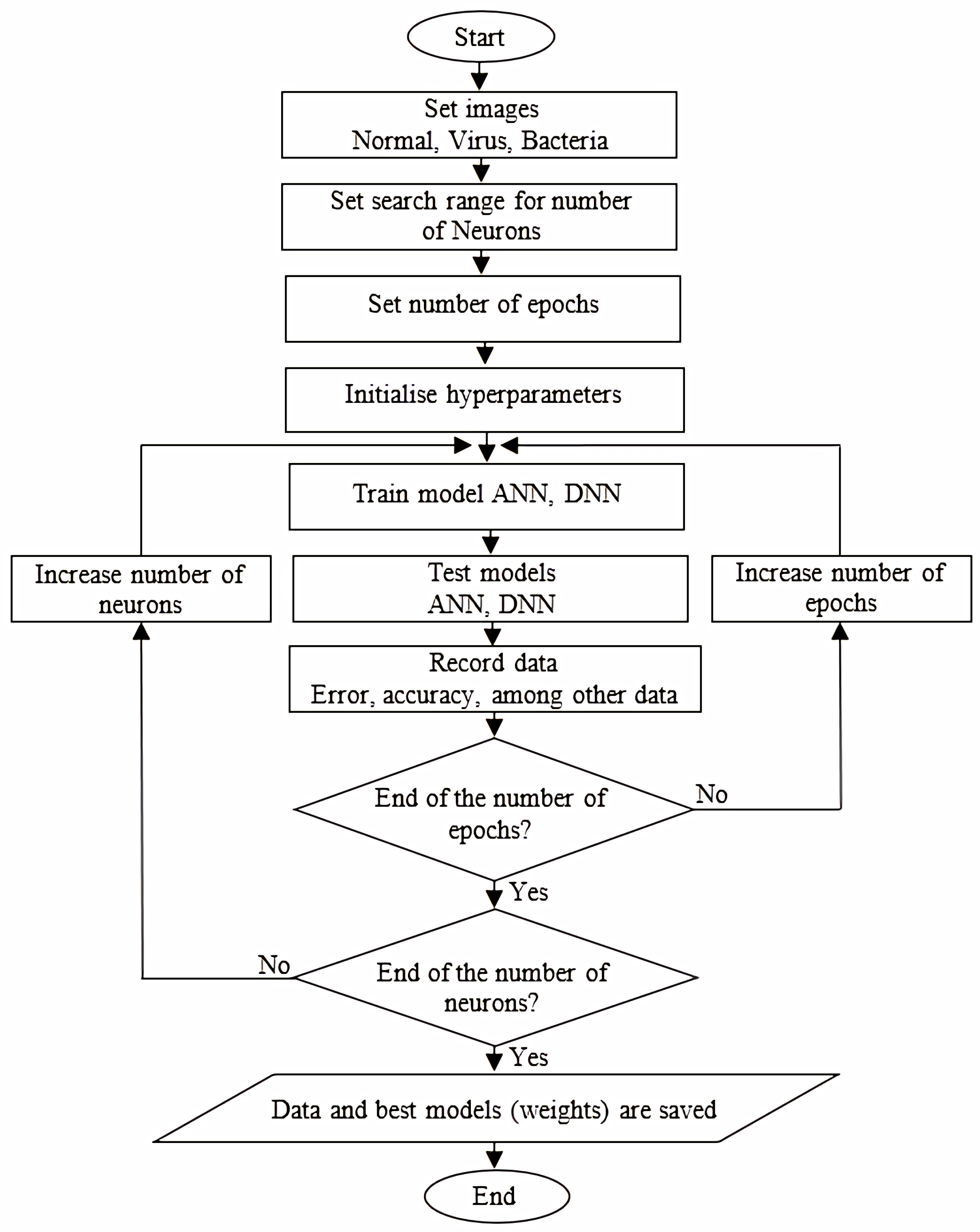
To address this issue, an exploratory experiment was conducted aiming to find the optimal number of neurons in the hidden layer, varying this parameter from 10 to 500 neurons. The increments were made in intervals of 10 neurons up to the first 100 neurons and increments of 50 neurons thereafter. Each increase in the number of neurons was accompanied by training epochs ranging from 1 to 100. For a clearer understanding of the experiment, Figure 9 can be referred to, which depicts the flowchart. With each increase in neurons and epochs, information was gathered to analyze the generated models. Additionally, experiments were conducted with both balanced and unbalanced data, seeking optimal cases for each package from among 1900 possibilities.
Table 1 presents a summary of the outstanding results, focusing on the overall accuracy achieved in the training set as the primary evaluation criterion. These results are detailed in Column 6. Additional training details are observed in Columns 2, 3, 4, and 5, such as the search range established to determine the number of neurons in the hidden layer, the type of dataset used (whether balanced or imbalanced), the specific number of neurons set to achieve the best result, and the training epochs, respectively.
It should be noted that when analyzing different packages, the overall accuracy in the training set is consistently higher when the dataset is unbalanced. Contrast Columns 1, 3, and 6 of Table 1 to verify this. As mentioned in Section 2.5, the overall accuracy during training reflects how well patterns from the training data have been captured by the model, although it may not provide information on the model’s performance on new data.
Analyzing the models’ performance on new data, one can observe the overall accuracy in the test set in Column 7, indicating that it is also consistently higher when the dataset is unbalanced. In this initial experiment, it is evident that the best-performing model was generated using the Keras package with convolutional layers, achieving an 80% overall accuracy on new data. While this value is respectable, it does not truly inform about the model’s performance concerning the individual classes present. In other words, an 80% overall accuracy on new (test) data suggests that out of every 100 samples analyzed by the model, 80 were correctly predicted. However, the following crucial question arises: does this hold true for all samples? According to the results obtained in this initial experiment, it becomes apparent that this is not the case.
To demonstrate this, the total number of processed labels during testing, as well as the number of actual and predicted labels for samples of normal (N) pathologies, viruses (V), and bacteria (B), are recorded from Column 8 to Column 15. Based on the provided information, the Keras package is analyzed in its implementation version for convolutional layers (see keras_cnn in Row 11 of Table 1), where an 80% overall accuracy in testing has been achieved. However, this model predicted 380 samples with normal labels when there were actually 373. It also predicted 90 and 167 samples with virus and bacteria labels, respectively, when there are actually 118 and 146 of each. These results do not align adequately with the observed overall accuracy of 80% in the tests, as there would be an expectation to see 298, 94, and 116 respective samples for the labels involved.
While the initial analysis focuses on the highest-performing model, the assessment of alternative models reveals that the overall accuracy achieved in tests does not provide a comprehensive representation of predictive performance by class. Referencing the Deepnet package, which achieves an overall accuracy of 65% in evaluations (see Deepnet in Row 2 of Table 1), a predisposition towards identifying features associated with normal pathology samples is detected, resulting in 451 predictions for this category, despite there being only 373 actual samples. Furthermore, this model shows an inability to identify bacterial pathology samples, failing to predict any of the 146 samples belonging to this classification. This discrepancy between observed results and the indicated overall accuracy of 65% suggests that evaluation metrics do not adequately reflect specific predictive performance by category, with distributions of 242, 76, and 94 samples for the respective labels being expected.
Exploring more alternative models is feasible; however, the inclination towards ineffective predictions indicated by the overall accuracy will continue to be misleading. This stems from its fundamental inability to elaborate on the predictions made by the model for each class, a limitation consistently observed across all implementations with R packages. Additionally, a discrepancy has been noted in the results presented in Table 1, marked by figures that exceed the actual quantities of predicted labels. This phenomenon suggests the existence of underlying causes presented below:
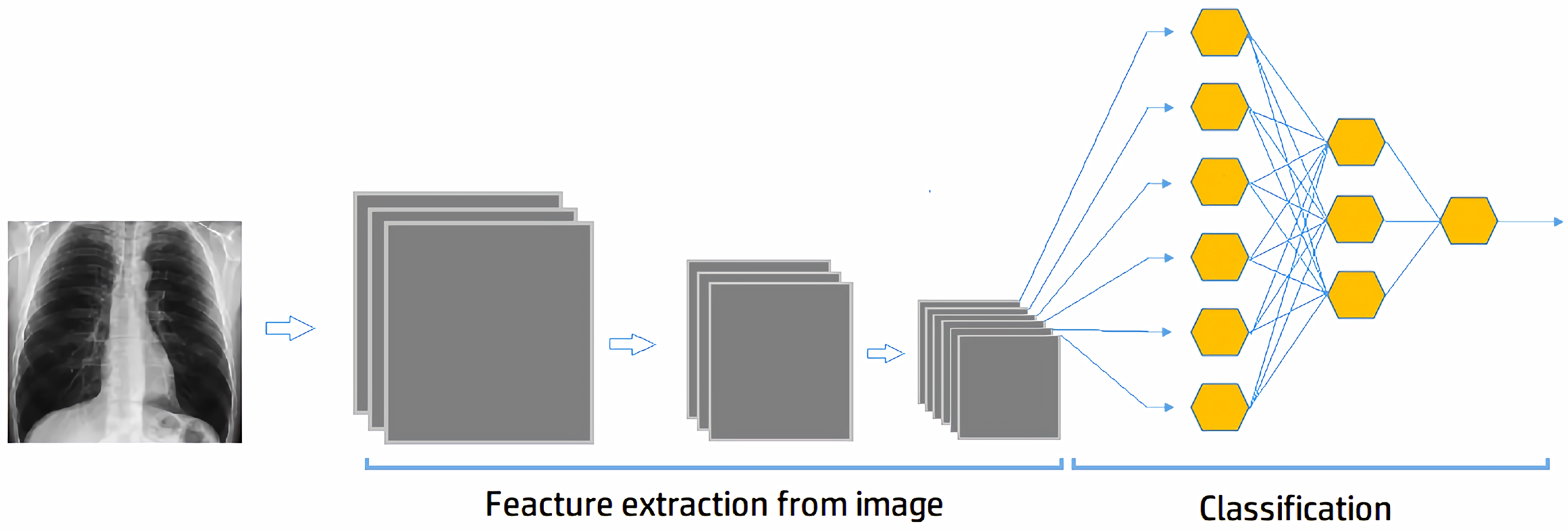
  • The number of dimensions handled per image. Despite preprocessing that reduces the image set to 900 features, it is high for certain neural networks, limiting their ability to map patterns effectively. However, improved mapping is observed for neural networks developed with the Keras package, especially when working with convolutional layers. In this case, pattern extraction is more efficient because convolutional layers do not specialize in individual pixels but rather in their spatial distribution, as discussed in Section 2.3.
  • The topology. The experiments in this first part involve only a single layer. This can be addressed by increasing the number of layers, which will be tested in subsequent phases.
  • The selection of hyperparameters. The neural networks handled by the various packages used in this work allow for the selection of multiple hyperparameters. To keep the experiments less complicated, tests were conducted with the default hyperparameter settings, and adjustments were made only in cases where contrasting results were not achieved or when the tests consumed a significant amount of time (see Section 2.4).
  • The established epochs for training. The pattern of inefficient predictions observed in all models developed with the R packages may be a result of the limited training, which barely reaches 100 epochs in this initial experiment. During each epoch, the different neural networks need to process and extract information from the images to update their weights; however, 100 epochs may not be sufficient for this task. To address this limitation, subsequent experiments will involve training the best-performing models with more epochs to achieve more robust results.
  • The number of neurons per layer. Not only the number of layers or topology, as it is often called, can affect the effectiveness of a neural network, but also the number of neurons per layer. However, the optimal models for a single layer have already been presented in Table 1, where the number of neurons can be observed in Column 4.
  • The dataset used. In the introduction, it has been noted that the dataset can significantly impact the model’s performance, including class balance. In this initial experiment, these variables have been controlled. Although the dataset was initially unbalanced, during preprocessing, the quantities of images per class were equalized. The summary in Table 1, particularly in Columns 3, 6, and 7, enables a comparison to understand the data balance’s influence.
Based on the preliminary discussion and the data from Table 1, a second experiment is conducted using the best models, selected based on the highest values of overall accuracy in both the training and testing sets (see Columns 6 and 7 of Table 1). This entails considering only the models trained with unbalanced datasets (see Column 3 of Table 1). However, not all selected models allowed for the second experiment, so their results are not displayed in Table 2.
Table 2 summarizes the data obtained after 1000 training epochs and testing for these models. The model selected from Table 1 and the overall accuracy achieved after completing the 1000 training epochs are shown in Columns 1 and 6, respectively. An increase in overall training accuracy is observed in all models. Regarding overall test accuracy, the Keras_30, Keras_150, and Keras_cnn_40 models show improvements, Kera_cnn_450 remains unchanged, and Neuralnet_100 experiences a 2-point decline. However, upon analyzing the record from Columns 8 to 16, an improvement in some classes is reflected, although it is noted that overall accuracy in testing does not truly reflect the model’s performance in relation to the individual classes present.
This is confirmed in Table 3, where metrics per class obtained from the testing data after completing the 1000 training epochs are presented. These metrics are derived from the confusion matrix introduced in Section 2.5 using the Caret package in R. In Table 3, from Columns 8 to 15, sensitivity, specificity, and precision metrics are shown for each class normal (N), virus (V), and bacteria (B), respectively.
The analysis of these metrics reveals a bias in the models’ prediction towards the normal class, demonstrated by higher sensitivity and precision for this class, while specificity is more conservative.
A deeper analysis of the overall accuracy in tests reveals its limitation in reflecting the performance of class-specific predictions for each model, as demonstrated by cross-referencing data from Table 1 and Table 2, which are detailed in Table 4. This table includes, in its first two Columns, the evaluated models and their respective training epochs, while the third column displays the overall accuracy in tests for each model. Columns 4, 7, and 10 detail the actual quantities of labels per class, and Columns 5, 8, and 11 present the class label estimates derived from the overall test accuracy. Considering the keras_30 model (see Row 1 of Table 4), with an overall accuracy of 71%, one would expect approximately 264, 83, and 103 samples for the classes of normal (N), virus (V), and bacteria (B) samples, respectively. However, Columns 6 and 9 reveal that this model predicted 450 and 187 samples for the N and V classes, respectively, and made no predictions for the B class, as shown in Column 12. The percentages contrasting overall test accuracy against class-specific accuracy are examined in Columns 13 to 18, providing a detailed perspective on the observed discrepancies.
An additional example highlighting the limited capability of overall test accuracy to reflect class-specific performance is observed in the keras_cnn_40 model (see Row 7 of Table 4). Upon analyzing this model, which achieves an overall accuracy of 81% in tests, Table 4 provides estimates of 302, 95, and 118 samples for the examined classes based on their respective quantities. However, the actual predictions per class are 359, 67, and 92. Therefore, it would be inaccurate to claim that this model achieves an 81% accuracy in class prediction, as the actual class-specific prediction percentages are 96.25%, 56.78%, and 63.01%, thus demonstrating the limitations of using a global metric as an indicator of detailed class performance.
This analysis concludes by highlighting a significant discrepancy between the overall accuracy in tests and the class-specific accuracy within models. It is emphasized that a high level of overall accuracy does not necessarily ensure equitable performance across all classes. Models exhibit considerable variability in predicting labels for specific classes, suggesting that overall accuracy might mask significant shortcomings in class-specific accuracy. Additionally, phenomena such as overfitting and targeted improvements in the prediction of particular classes are not necessarily reflected in the overall accuracy. This underscores the importance of conducting a detailed evaluation of class-specific performance to gain a comprehensive understanding of a model’s effectiveness, particularly in situations where maintaining a balance among classes is crucial.

3.2. Results and Analysis for Two Layers

In this exploratory experiment, an additional layer is introduced to create a two-layer structure within the topology. Unlike the previous experiments detailed in Section 3.1, Deepnet is excluded here due to its inability to produce results comparable to other packages. This limitation stems from its incapacity to handle the 900 features (dimensions) remaining after image preprocessing. Consequently, the evaluation is narrowed down to the Neuralnet, RSNNS, and Keras packages. The aim is to achieve high accuracy values in both training and testing, which requires determining the optimal combination of the number of neurons per layer, ranging from 50 to 300 in increments of 50 neurons. A total of 100 training epochs are maintained for each combination of neurons in the layers, and then the collected information is analyzed.
In contrast to the first experiment, the search is restricted to 36 cases per R package for both balanced and unbalanced data. Table 5 provides a summary of the best results found over 100 training epochs, including an additional column for the neurons in the second layer for each model. A slight improvement in overall accuracy is observed in the training set for some models, but it remains consistently higher when the data are unbalanced.
Regarding the accuracy in the test set, it does not reveal a significant improvement compared to the previous scenario, except for some models. For this reason, the best models undergo an additional 1000 epochs of training. A summary of the information obtained, including the metrics of interest, is presented in Table 6.
Again, the overall accuracy in training after 1000 epochs corresponds to models implemented with unbalanced data, with those implemented using the Keras package, including its two models with convolutional layers being better (see Column 7, Rows 2, 4, and 5 of Table 6). As for the test accuracy, the best model achieves 79%, which is keras_cnn_100_150 implemented with convolutional layers.
For this overall accuracy value in tests or any other reported in Table 6, it is feasible to apply an analysis similar to the one conducted in Section 3.1. This analysis demonstrates the limited informative capacity of this global metric to reflect class-specific sample predictions. For instance, based on the expectation generated by a 79% accuracy in tests, one would anticipate 294, 93, and 115 samples, respectively, for each assessed class. However, as detailed class accuracy in Row 4, Columns 15, 16, and 17 of Table 6 indicates, the actual predictions reach 96%, 52%, and 58%, corresponding to 358, 61, and 84 predicted samples, respectively, for the involved classes. This discrepancy from the estimates provided by the global accuracy underscores, once again, that global metrics do not provide a faithful overview of class-specific predictions of a trained model.
The analysis of overall accuracy versus class-specific accuracy in models such as keras_250_300 and keras_cnn_100_150 reveals a significant contrast, with high success rates in training that do not directly translate into effective generalization during testing, where accuracy notably decreases. This phenomenon is accentuated when examining class-specific accuracy, where despite high percentages being achieved in class N, classes V and B display considerably lower accuracies, highlighting inequalities in the model’s predictive capability. Furthermore, the comparison between models trained with balanced and unbalanced data indicates that although data balancing may not optimize overall accuracy, it promotes a fairer distribution in the detection of all classes, improving equity in classification. Sensitivity and specificity by class complement this picture, showing that a high ability to identify true negatives does not necessarily ensure equitable detection of all positive classes, underscoring the need for strategies that promote balanced and effective performance in class-specific classification of the developed models.

3.3. Results and Analysis of Layers Three and Four

In these experiments, a comprehensive exploration of the Neuralnet, RSNNS, and Keras packages is conducted to identify the most effective model in terms of 3 and 4-layer topologies, focusing exclusively on the unbalanced dataset. In accordance with the methodology of prior experiments, the aim is to achieve the optimal neuron configuration in each layer to attain high accuracy in both training and testing phases by adjusting this parameter across a range from 50 to 300, with increments of 50 neurons. These experiments examine 216 and 1296 possible cases for 3 and 4 layers, respectively.
After completing 100 training epochs for each combination of neurons in the 3 and 4-layer topologies, meticulous data collection was carried out for subsequent analysis. The best models were selected at the end of the 100 epochs and subjected to additional training of 1000 and 3000 epochs. A summary of the metrics obtained is shown in Table 7 and Table 8, along with the results of the 2-layer topology for comprehensive comparison. It is important to mention that the Neuralnet and RSNNS packages only completed 100 and 200 training epochs, respectively, so they are labeled as only_100 and only_200 in the epoch column in the tables because they did not show significant improvements with an additional 1000 epochs.
A comprehensive evaluation of models trained with 1000 and 3000 epochs reveals crucial insights into the balance between fitting to training data and generalizing to unseen data sets. Primarily, it is observed that increasing the number of epochs improves accuracy during training; however, this improvement is not proportionally reflected in the accuracy of tests, indicating a tendency towards overfitting in extensively trained models. Specifically, sensitivity by class tends to increase slightly with more training epochs for class N, although classes V and B continue to experience relatively low sensitivities, highlighting persistent challenges in impartial classification across all categories.
Furthermore, the high specificity in all models, regardless of the number of epochs, suggests a robust competence in correctly identifying true negatives. However, accuracy by class does not show significant improvements with the increase in epochs, underlining that effective detection of true negatives does not directly translate into an enhanced ability to accurately classify all classes.
Crucially, the model architecture, especially the inclusion of convolutional layers and a balanced distribution of neurons in the keras_cnn models, stands out as a determinant factor in effective generalization. This finding highlights the importance of optimal model architecture and suggests that appropriate neuronal configuration strategies are essential for enhancing the overall performance of the model.
The analysis also underscores that a greater number of training epochs does not necessarily guarantee an improvement in the capacity for generalization, highlighting the challenge of overfitting, especially in models trained for 3000 epochs. This emphasizes the need to adopt a nuanced approach in model design and in the implementation of effective strategies to combat overfitting.
Finally, the importance of meticulously balancing the fit to training data with the ability to effectively generalize to new data is highlighted. Optimizing the model architecture, including the strategic selection of convolutional layers and neuronal configuration, along with a careful approach to training duration, emerges as crucial for achieving optimal performance. This synthesis of findings emphasizes the relevance of a detailed and holistic evaluation of model performance, which goes beyond overall accuracy to include sensitivity, specificity, and accuracy by class, thus ensuring robust and equitable classification systems.

3.4. Additional Results and Analysis

In Section 3.2 and Section 3.3, a comprehensive analysis of the Neuralnet, RSNNS, and Keras packages was conducted to determine the most effective model for 2, 3, and 4-layer topologies, with a specific focus on imbalanced datasets. The optimal combination of neurons in each layer was sought, varying this parameter between 50 and 300. Neuron combinations in the range of 10 to 40 were excluded from these experiments, although some results in Table 1 for the Keras and Neuralnet packages showed models with 30, 40, and even 10 neurons (see rows 6, 10, and 14 in Table 1). For this reason, additional experiments were conducted within this range to determine if superior models to those previously discussed could be obtained. These experiments were carried out using the Neuralnet, Keras, and RSNNS packages. Despite RSNNS initially not producing models with few neurons, it was included in the analysis. The results of these additional experiments are detailed in Table 9, from which the following conclusions are drawn.
The analysis of the data suggests a disparity between training accuracy and test accuracy, yet it shows a strong inclination to corroborate previous findings. This is highlighted by the wide variability in training accuracy, ranging from 56% to 96%, as opposed to the narrower test accuracy range of 54% to 82%. This pattern underscores a tendency towards overfitting in certain configurations, where excessive optimization on training data undermines the model’s effectiveness with new samples.
The detailed examination of the overall accuracy in tests once again confirms the limitation of this global metric in accurately projecting class-specific prediction estimates. This is demonstrated by observing the accuracy per class, highlighting the challenges that models face in achieving a uniform classification across all categories. In Table 3 and Table 6, Table 7, Table 8 and Table 9, it is observed that a high overall test accuracy does not necessarily translate into high test accuracy across all classes. Table 10 provides a contrast between the overall test accuracy and the test accuracy per class for the most outstanding models that employ keras with convolutional layers (keras_cnn). The data in Columns 1, 2, and 3 allow for the verification of information corresponding to the table, row, and column. It is reported that the overall test accuracy for these selected models ranges from 79% to 82%.
However, a detailed inspection of accuracy per class (N, V, and B) reveals more pronounced variations. Class N proves to be robust across all models, which could indicate adequate representation or clearer distinction of its characteristics within the dataset. In contrast, classes V and B exhibit lower and more erratic performance, with class V achieving accuracies ranging from 51% to 59%, and class B from 58% to 70%, suggesting potential challenges related to data representativeness or the keras_cnn model’s ability to capture the specific features of these classes. Despite the prior knowledge of the number of samples per class, these results reflect the existing imbalance in the training data. The consistency of high accuracy for class N, as opposed to the variability for classes V and B, points to a potential model bias toward class N. Given the stability of the overall accuracy, it could be inferred that class N is predominant in the datasets, which could lead to misguided conclusions about the model’s overall effectiveness.
Class sensitivity highlights significant differences, consistently demonstrating superior effectiveness in identifying positive cases, especially for class N, in models that incorporate convolutional layers (keras_cnn). On the other hand, specificity remains high across all models, showcasing an efficient ability to correctly recognize true negatives.
Regarding neuron configuration, models based on artificial neural network algorithms typically exhibit lower accuracy with fewer neurons. However, the four-layer Neuralnet model achieves a slight edge in precision over its counterparts. For deep-learning models subjected to 1000 epochs of training, the resulting accuracy remains consistent, unaffected by the number of neurons deployed.
Concluding with the number of training epochs, it is observed that models trained for 1000 epochs generally exhibit a better balance between accuracy in training and testing than those trained for only 100 or 200 epochs.

4. Discussion

The presented research comprehensively addresses the impact of sample imbalance and the configuration of neural network-based models on the reporting capability of metrics used in the classification of pulmonary pathologies. In this regard, experiments were conducted to evaluate classification models under various neuronal configurations and data balance conditions. The central premise was to examine how these variables affect the global accuracy and class-specific performance of the models in detecting pulmonary pathologies from images.
In the initial exploration for a single layer, selecting the optimal number of neurons emerged as a critical challenge to achieve high accuracy in training and testing. The findings highlight the complexity of adjusting the network topology to optimize performance, suggesting there is no single rule for neuron configuration that guarantees success. Interestingly, results indicate that models with unbalanced datasets tend to show higher accuracy in training, though this phenomenon does not necessarily translate into improved generalization capability on new data.
When analyzing performance on test datasets, it was revealed that global accuracy does not adequately reflect the model’s performance with respect to individual classes. Particularly in high-performing models, such as those implemented with the Keras package and its variants with convolutional layers, significant discrepancies were observed in class-specific accuracy. This underscores the importance of looking beyond global metrics to understand the model’s behavior in classifying different types of pathologies.
The inclusion of additional layers in subsequent experiments provided an opportunity to investigate the influence of more complex topologies on model effectiveness. While marginal improvements in accuracy were observed with the addition of layers, the persistence of data imbalance as a critical factor in evaluating global and class-specific accuracy remained. Models trained with 1000 or more epochs showed improvements in training accuracy, highlighting the need for a holistic approach to training and evaluating the models’ generalization capabilities.
The discussion on the informative capacity of global metrics highlights an inherent limitation in capturing the true performance of models in classifying different categories. This aspect is critical, especially in medical applications where accuracy in detecting specific pathologies is paramount.
With the proposed data preprocessing techniques, the implemented models are close to the results reported in many previous studies for the same dataset. Assuming the results presented in [26] are associated with test sets, they report an accuracy of 85% with a sensitivity of 84.1%. While these results are very close to this study, they do not address the problems demonstrated in this study. Nor do they detail the effect of classes individually. The work of [26] rather merges the virus and bacteria classes, which can be counterproductive as it may hide potential biases in the final results [51].
It is crucial to prevent the spread of errors among classes. Thus, a class-specific analysis, as conducted in this study, is recommended, demonstrating that individual classes impact model performance. Indeed, the sensitivity value indicates that the model correctly identifies the positive class, typically pneumonia cases, 84.1% of the time, suggesting that 84.1% may correspond to a viral or bacterial pathology. However, this value is not truly representative of either class because the original dataset is imbalanced, with a significantly larger number of samples in the normal class, leading to bias if the training is not carefully managed. Notably, in many instances, sensitivity may appear high, as in the work of [26] where classes are merged, but taking the best model implemented with the Keras package using convolutional layers, a much lower combined sensitivity of approximately 70% is observed than shown in this work. This calculated measure of combined sensitivity is not standard but draws attention to the results presented in many studies when classes are merged, and the impact of the involved classes is not detailed, especially if they are imbalanced.
This research is also compared to the analysis conducted by [14], which examines lung images affected by tuberculosis and pneumonia, as well as those of healthy individuals, focusing on the equitable use of 306 samples per category, data augmentation techniques, and the application of deep neural networks through transfer learning. Although the [14] study reports high AUC scores of 90%, 93%, and 99% for the respective categories, a potential bias is identified from grouping all pneumonia cases into a single class without considering their distinct viral or bacterial causes. This approach could limit the accuracy of the training by overlooking specific patterns during feature extraction, as suggested by [26]. In contrast, the current study favors metrics derived from the confusion matrix, which offers greater sensitivity to class imbalance. Furthermore, it is highlighted that models trained with balanced data show significantly lower performance compared to those obtained with imbalanced data, suggesting that the impressive AUC values reported by [14] might not adequately reflect effective discrimination between classes.
In the study [9], significant progress is highlighted in the field of medical image retrieval, particularly focusing on the identification of pulmonary pathologies through common image signs found in computed tomographies. The research underscores how the inclusion of contextual and semantic analysis, along with visual characteristics, significantly contributes to improved precision in finding relevant images. This is demonstrated by an increase in the MAP from 60% to 70% and an improvement in the AUC from 0.48 to 0.58. The findings emphasize the drawback of relying solely on visual characteristics. Delving deeper into the details of this study, it is evident that grouping distinctive features of the examined pathologies can decrease the precision of training by overlooking specific patterns during the feature extraction process.
The comparison between preprocessing methodologies implemented in previous studies and the research presented illustrates significant variations in approaches and technical procedures, especially in the context of analyzing X-ray images for the detection of pulmonary diseases. The referenced studies, including [9,14,26], establish a methodological basis for the preprocessing of medical images, while the research under discussion introduces detailed techniques aimed at overcoming specific challenges, such as the dimensional variability of the images and class balance.
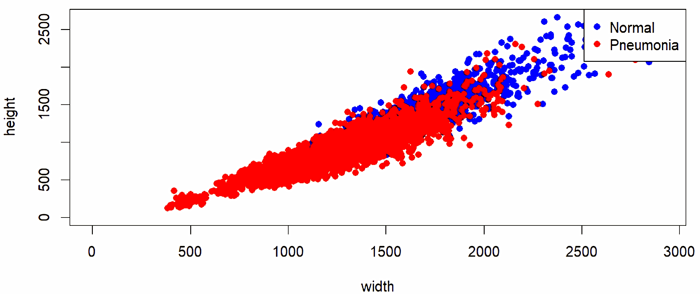
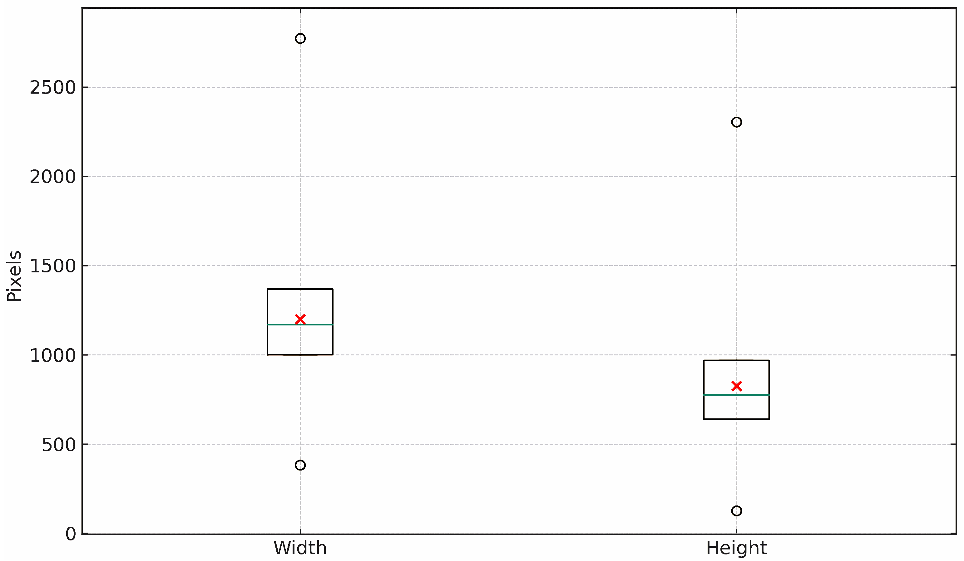
Regarding selection and resizing, the adoption of selection criteria based on specific dimensions (>1000 pixels) is emphasized to prevent deformations during resizing, a step not mentioned in previous studies. This method ensures the preservation of relevant information through standardized cropping to 1000 × 1000 pixels and further reduction to 30 × 30 pixels, therefore optimizing the uniformity and quality of the images for subsequent analysis.
Regarding the application of statistical analysis and class balance, the research incorporates statistical analysis to guide image selection, in contrast to the more generalized methodologies of previous studies. This analysis enables informed selection, enhancing the representativeness of the dataset. The formation of balanced and imbalanced sets directly addresses the impact of class balance on the effectiveness of the classification model, an aspect not always explicitly dealt with in the compared studies.
The review of studies highlights significant deficiencies in considering the differential impact of classes and specific patterns during the feature extraction phases, underscoring the lack of detailed analysis on the influence of classes and common image signs. This omission points to a critical need for more detailed classificatory evaluations to ensure precise and balanced interpretations in the classification of pulmonary diseases. The importance of a holistic approach that prioritizes the optimization of architectures and the calibration of the training period for improved generalization becomes evident. Furthermore, the need for adaptive and meticulous preprocessing of medical images to address challenges such as dimensional variability and class imbalance is emphasized. The current research underlines the relevance of customizing preprocessing techniques and conducting a model performance analysis that includes sensitivity, specificity, and class precision. This directs towards the development of more robust and equitable classification models, urging future research to establish clear guidelines for hyperparameter tuning and neural network architectures, therefore facilitating significant advances in the application of deep-learning technologies for medical diagnosis.

5. Conclusions

In this study, the development of classification models using both artificial neural networks and deep neural networks for categorizing clinically related pathology images was explored. The implementation of these models was carried out using R packages, specifically Keras, Neuralnet, RSNNS, Deepnet, and nnet.
The main objective of the study was to demonstrate how sample imbalance in lung pathology-related images can significantly affect the informativeness of metrics derived from the confusion matrix for all implemented classification models.
According to the results obtained from the explored models, it is observed that the overall prediction-related metric, both in training and testing, can be high but lacks informativeness. This is demonstrated in the class-specific metrics, where substantially higher sensitivity and precision are observed for the normal class compared to the virus and bacteria classes, reflecting the impact of class imbalance in the dataset on the implemented models. Although the specificity metric is high in all implemented classification models, this value is not sufficient to claim that the models in question are accurate in their predictions.
These results raise questions about the procedures used to group classes in many studies, aiming to achieve class balance in imbalanced data and open new avenues for future research to investigate the impact of class separation in datasets with clinical pathologies. The purpose is to better understand how to extract specific features from each category with greater precision and, thus, improve the efficiency of these models.

Author Contributions

Conceptualization, A.A.O. and C.J.H.; methodology, A.A.O. and C.J.H.; software, A.A.O.; validation, A.A.O., C.J.H., A.T. and J.G.; writing—original draft preparation, A.A.O. and C.J.H.; writing—review and editing, A.V., M.L.-B., A.T. and J.G.; supervision, A.T.; funding acquisition, J.G. All authors have read and agreed to the published version of the manuscript.

Funding

This work was supported by the program “Programa de Estímulo a la Excelencia para Profesorado Universitario Permanente” of the Vice Rectorate for Research and Knowledge Transfer of the University of Alcala and by the Comunidad de Madrid (Spain) through project EPU-INV/2020/004.

Informed Consent Statement

Not applicable.

Data Availability Statement

The selected dataset in this study is available on this link: https://www.kaggle.com/paultimothymooney/chest-xray-pneumonia (accessed on 1 April 2024).

Conflicts of Interest

The authors declare no conflicts of interest.

Abbreviations

The following abbreviations are used in this manuscript:
CNNConvolutional Neural Network
SNNSStuttgart Neural Network Simulator
DBNDeep Belief Network
ReLURectified Linear Unit

References

  1. Ponce, P. Inteligencia Artificial: Con Aplicaciones a la Ingeniería; Alpha Editorial: Bogota, Colombia, 2010. [Google Scholar]
  2. Vogt, M. An overview of deep learning and its applications. In Proceedings of the Fahrerassistenzsysteme 2018: Von der Assistenz zum automatisierten Fahren 4. Internationale ATZ-Fachtagung Automatisiertes Fahren, Wiesbaden, Germany, 18–19 April 2018; pp. 178–202. [Google Scholar]
  3. Russell, S.J.; Norvig, P. Artificial Intelligence a Modern Approach; Pearson: London, UK, 2010. [Google Scholar]
  4. Mishra, R.K.; Reddy, G.Y.S.; Pathak, H. The Understanding of Deep Learning: A Comprehensive Review. Math. Probl. Eng. 2021, 2021, 5548884. [Google Scholar] [CrossRef]
  5. Bianchini, M.; Scarselli, F. On the Complexity of Neural Network Classifiers: A Comparison Between Shallow and Deep Architectures. IEEE Trans. Neural Networks Learn. Syst. 2014, 25, 1553–1565. [Google Scholar] [CrossRef] [PubMed]
  6. Buduma, N.; Locascio, N. Fundamentals of Deep Learning; O’Rreilly: Springfield, MO, USA, 2017. [Google Scholar]
  7. Boehmke, B.; Greenwell, B.M. Hands-on Machine Learning with R; CRC Press: Boca Raton, FL, USA, 2019. [Google Scholar]
  8. Moshayedi, A.J.; Roy, A.S.; Kolahdooz, A.; Shuxin, Y. Deep Learning Application Pros And Cons Over Algorithm. EAI Endorsed Trans. Robot. 2022, 22, 7. [Google Scholar] [CrossRef]
  9. Kashif, M.; Raja, G.; Shaukat, F. An Efficient Content-Based Image Retrieval System for the Diagnosis of Lung Diseases. J. Digit. Imaging 2020, 33, 971–987. [Google Scholar] [CrossRef] [PubMed]
  10. Müller, D.; Soto-Rey, I.; Kramer, F. Towards a guideline for evaluation metrics in medical image segmentation. BMC Res. Notes 2022, 15, 210. [Google Scholar] [CrossRef]
  11. Djavanshir, G.R.; Chen, X.; Yang, W. A Review of Artificial Intelligence’s Neural Networks (Deep Learning) Applications in Medical Diagnosis and Prediction. IT Prof. 2021, 23, 58–62. [Google Scholar] [CrossRef]
  12. Kim, M.; Yun, J.; Cho, Y.; Shin, K.; Jang, R.; Bae, H.j.; Kim, N. Deep learning in medical imaging. Neurospine 2019, 16, 657. [Google Scholar]
  13. Greeshma, K.; Viji Gripsy, J. A review on classification and retrieval of biomedical images using artificial intelligence. In The Fusion of Internet of Things, Artificial Intelligence, and Cloud Computing in Health Care; Springer: Berlin/Heidelberg, Germany, 2021; pp. 47–66. [Google Scholar]
  14. Zak, M.; Krzyżak, A. Classification of Lung Diseases Using Deep Learning Models. In Proceedings of the International Conference on Computational Science, Amsterdam, The Netherlands, 3–5 June 2020; Volume 12139, pp. 621–634. [Google Scholar]
  15. Pommé, L.E.; Bourqui, R.; Giot, R.; Auber, D. Relative Confusion Matrix: Efficient Comparison of Decision Models. In Proceedings of the 2022 26th International Conference Information Visualisation (IV), Vienna, Austria, 19–22 July 2022; pp. 98–103. [Google Scholar]
  16. Ochella, S.; Shafiee, M. Performance Metrics for Artificial Intelligence (AI) Algorithms Adopted in Prognostics and Health Management (PHM) of Mechanical Systems. J. Phys. Conf. Ser. 2021, 1828, 012005. [Google Scholar] [CrossRef]
  17. Blagec, K.; Dorffner, G.; Moradi, M.; Samwald, M. A critical analysis of metrics used for measuring progress in artificial intelligence. arXiv 2020, arXiv:2008.02577. [Google Scholar]
  18. Rustam, Z.; Purwanto, A.M.D.C.; Hartini, S.; Saragih, G.S. Lung cancer classification using fuzzy c-means and fuzzy kernel C-Means based on CT scan image. IAES Int. J. Artif. Intell. 2021, 10, 291–297. [Google Scholar] [CrossRef]
  19. Sugimori, H.; Shimizu, K.; Makita, H.; Suzuki, M.; Konno, S. A Comparative Evaluation of Computed Tomography Images for the Classification of Spirometric Severity of the Chronic Obstructive Pulmonary Disease with Deep Learning. Diagnostics 2021, 11, 929. [Google Scholar] [CrossRef]
  20. Yadlapalli, P.; Bhavana, D.; Suryanarayana, G. Intelligent classification of lung malignancies using deep learning techniques. Int. J. Intell. Comput. Cybern. 2021, 15, 345–362. [Google Scholar] [CrossRef]
  21. Mridha, M.F.; Prodeep, A.R.; Hoque, A.S.M.M.; Islam, M.R.; Lima, A.A.; Kabir, M.M.; Hamid, M.A.; Watanobe, Y. A Comprehensive Survey on the Progress, Process, and Challenges of Lung Cancer Detection and Classification. J. Healthc. Eng. 2022, 2022. [Google Scholar] [CrossRef]
  22. Albahri, O.S.; Zaidan, A.A.; Albahri, A.S.; Zaidan, B.B.; Abdulkareem, K.H.; Al-qaysi, Z.T.; Alamoodi, A.H.; Aleesa, A.M.; Chyad, M.A.; Alesa, R.; et al. Systematic review of artificial intelligence techniques in the detection and classification of COVID-19 medical images in terms of evaluation and benchmarking: Taxonomy analysis, challenges, future solutions and methodological aspects. J. Infect. Public Health 2020, 13, 1381–1396. [Google Scholar] [CrossRef]
  23. David, J.; Krishnan, R.; Kumar, S. Neural network based retinal image analysis. In Proceedings of the 2008 Congress on image and Signal Processing, Sanya, China, 27–30 May 2008; IEEE: Piscataway, NJ, USA, 2008; Volume 2, pp. 49–53. [Google Scholar]
  24. Montoya, Y.A.C.; Cornejo, S.A.G. Detección de COVID-19 a partir de imágenes radiográficas utilizando redes neuronales convolucionales: Una revisión bibliográfica. INGENIERÍA INVESTIGA 2022, 4. [Google Scholar] [CrossRef]
  25. Choy, S.P.; Kim, B.J.; Paolino, A.; Tan, W.R.; Lim, S.M.L.; Seo, J.; Tan, S.P.; Francis, L.; Tsakok, T.; Simpson, M.; et al. Systematic review of deep learning image analyses for the diagnosis and monitoring of skin disease. NPJ Digit. Med. 2023, 6, 180. [Google Scholar] [CrossRef]
  26. Yee, S.L.K.; Raymond, W.J.K. Uah. In Proceedings of the 2020 10th International Conference on Biomedical Engineering and Technology, Tokyo, Japan, 15–18 September 2020. [Google Scholar]
  27. Chest-Xray-Pneumonia. Available online: https://www.kaggle.com/datasets/paultimothymooney/chest-xray-pneumonia (accessed on 3 March 2024).
  28. Han, G.; Liu, X.; Han, F.; Santika, I.N.T.; Zhao, Y.; Zhao, X.; Zhou, C. The LISS—A public database of common imaging signs of lung diseases for computer-aided detection and diagnosis research and medical education. IEEE Trans. Biomed. Eng. 2014, 62, 648–656. [Google Scholar] [CrossRef]
  29. Das, S.; Pradhan, S.K.; Mishra, S.; Pradhan, S.; Pattnaik, P.K. A Machine Learning based Approach for Detection of Pneumonia by Analyzing Chest X-Ray Images. In Proceedings of the 2022 9th International Conference on Computing for Sustainable Global Development (INDIACom), New Delhi, India, 23–25 March 2022; pp. 177–183. [Google Scholar]
  30. Ciaburro, G.; Venkateswaran, B. Neural Networks with R: Smart Models Using CNN, RNN, Deep Learning, and Artificial Intelligence Principles; Packt Publishing: Birmingham, UK, 2017. [Google Scholar]
  31. Machart, P.; Ralaivola, L. Confusion Matrix Stability Bounds for Multiclass Classification. arXiv 2012, arXiv:1202.6221. [Google Scholar]
  32. Handelman, G.S.; Kok, H.K.; Chandra, R.V.; Razavi, A.H.; Huang, S.; Brooks, M.; Lee, M.J.; Asadi, H. Peering into the black box of artificial intelligence: Evaluation metrics of machine learning methods. Am. J. Roentgenol. 2019, 212, 38–43. [Google Scholar] [CrossRef]
  33. Reinke, A.; Maier-Hein, L.; Müller, H. Common limitations of performance metrics in biomedical image analysis. In Proceedings of the Medical Imaging with Deep Learning (MIDL 2021), Lübeck, Germany, 7–9 July 2021. [Google Scholar]
  34. McCulloch, W.S.; Pitts, W. A logical calculus of the ideas immanent in nerous activity. Bull. Math. Biophys. 1943, 5, 115–133. [Google Scholar] [CrossRef]
  35. Liaw, J.S.; Berger, T.W. Dynamic synapse: A new concept of neural representation and computation. Hippocampus 1996, 6, 591–600. [Google Scholar] [CrossRef]
  36. Palm, G. Warren mcculloch and walter pitts: A logical calculus of the ideas immanent in nervous activity. In Proceedings of the Brain Theory: Proceedings of the First Trieste Meeting on Brain Theory, Trieste, Italy, 1–4 October 1984; Springer: Berlin/Heidelberg, Germany, 1986; pp. 229–230. [Google Scholar] [CrossRef]
  37. Stanley, K.O.; Miikkulainen, R. Evolving neural networks through augmenting topologies. Evol. Comput. 2002, 10, 99–127. [Google Scholar] [CrossRef] [PubMed]
  38. IBM Artificial Intelligence. Available online: https://developer.ibm.com/technologies/artificial-intelligence/ (accessed on 3 March 2024).
  39. Zhu, H.; An, Z.; Yang, C.; Xu, K.; Zhao, E.; Xu, Y. EENA: Efficient Evolution of Neural Architecture. In Proceedings of the 2019 IEEE/CVF International Conference on Computer Vision Workshop (ICCVW), Seoul, Republic of Korea, 27–28 October 2019; pp. 1891–1899. [Google Scholar] [CrossRef]
  40. Polson, N.G.; Sokolov, V.O. Deep Learning. arXiv 2018, arXiv:1807.07987. [Google Scholar]
  41. Hellín, C.J.; Valledor, A.; Cuadrado-Gallego, J.J.; Tayebi, A.; Gómez, J. A Comparative Study on R Packages for Text Mining. IEEE Access 2023, 11, 99083–99100. [Google Scholar] [CrossRef]
  42. Quintans-Júnior, L.J.; Gurgel, R.Q.; de Souza Araújo, A.A.; Correia, D.; Martins-Filho, P.R.S. ChatGPT: The new panacea of the academic world. Rev. Soc. Bras. Med. Trop. 2023, 56, e0060-2023. [Google Scholar] [CrossRef]
  43. RDocumentation. Available online: https://www.rdocumentation.org/ (accessed on 3 March 2024).
  44. MachineLearning. Available online: https://cran.r-project.org/web/views/MachineLearning.html (accessed on 1 March 2024).
  45. Bergmeir, C.; Benítez, J.M. Neural Networks in R Using the Stuttgart Neural Network Simulator: RSNNS. J. Stat. Softw. 2012, 46, 1–26. Available online: https://www.jstatsoft.org/index.php/jss/article/view/v046i07 (accessed on 17 April 2024). [CrossRef]
  46. Günther, F.; Fritsch, S. neuralnet: Training of Neural Networks. R J. 2010, 2, 30–38. [Google Scholar] [CrossRef]
  47. Rong, X. deepnet: Deep Learning Toolkit in R. R Package Version 0.2.1. 2022. Available online: https://CRAN.R-project.org/package=deepnet (accessed on 17 April 2024).
  48. Allaire, J.J.; Chollet, F. keras: R Interface to ’Keras’. R Package Version 2.13.0. 2023. Available online: https://CRAN.R-project.org/package=keras (accessed on 17 April 2024).
  49. Venables, W.N.; Ripley, B.D. Modern Applied Statistics with S, 4th ed.; Springer: New York, NY, USA, 2002; ISBN 0-387-95457-0. Available online: https://www.stats.ox.ac.uk/pub/MASS4/ (accessed on 17 April 2024).
  50. Kuhn, M. Max, Building Predictive Models in R Using the caret Package. J. Stat. Softw. 2008, 28, 1–26. Available online: https://www.jstatsoft.org/index.php/jss/article/view/v028i05 (accessed on 17 April 2024). [CrossRef]
  51. Beauxis-Aussalet, E.; Hardman, L. Visualization of Confusion Matrix for Non-Expert Users. In Proceedings of the IEEE Conference on Visual Analytics Science and Technology (VAST)-Poster Proceedings, Paris, France, 25–31 October 2014; pp. 1–2. [Google Scholar]
  52. Kermany, D.; Zhang, K.; Goldbaum, M. Labeled optical coherence tomography (oct) and chest x-ray images for classification. Mendeley Data 2018, 2, 651. [Google Scholar]
  53. Kermany, D.S.; Goldbaum, M.; Cai, W.; Valentim, C.C.; Liang, H.; Baxter, S.L.; McKeown, A.; Yang, G.; Wu, X.; Yan, F.; et al. Identifying medical diagnoses and treatable diseases by image-based deep learning. Cell 2018, 172, 1122–1131. [Google Scholar] [CrossRef]
Figure 1. Deep-learning architectures.
Applsci 14 03419 g001
Figure 2. Variables associated with the cost of a house as inputs in artificial neural networks.
Applsci 14 03419 g002
Figure 3. Variables associated with the pixels of an image as input in artificial neural networks.
Applsci 14 03419 g003
Figure 4. General architecture of a CNN.
Applsci 14 03419 g004
Figure 5. Comparison of the dimensions between normal versus pneumonia imaging sets.
Applsci 14 03419 g005
Figure 6. Statistics on width and height for set of images “normal”.
Applsci 14 03419 g006
Figure 7. Statistics on width and height for set of images “pneumonia”.
Applsci 14 03419 g007
Figure 8. Image preprocessing.
Applsci 14 03419 g008
Figure 9. Diagram for the development of models.
Applsci 14 03419 g009
Table 1. Summary of the data obtained for 100 training epochs with one layer and the testing of the different R packages.
PackageSearch RangeDatasetNumber NeuronsEpochAccuracy TrainAccuracy TestTotal LabelsLabels Actual NLabels Predicted NLabels Actual VLabels Predicted VLabels Actual BLabels Predicted BLabels not Predicted
deepnet10–100No_bal80640.650.65637373451118186146
deepnet100–500No_bal100990.640.64637373396118241146
deepnet10–100Bal80940.470.48354118105118249118
deepnet100–500Bal10040.330.33354118354118 118
keras10–100No_bal30850.700.71637373450118187146
keras100–500No_bal150770.670.68637373373118264146
keras10–100Bal100910.540.53354118145118209118
keras100–500Bal150890.550.54354118182118172118
keras-cnn10–100No_bal40880.890.7863737346211860146115
keras-cnn100–500No_bal450530.920.8063737338011890146167
keras-cnn10–100Bal30890.740.6335411815411816011840
keras-cnn100–500Bal150840.850.6335411891118111118152
neuralnet10–100No_bal10810.670.67637373393118173146683
neuralnet100–500No_bal100620.690.606373733171182431466611
neuralnet10–100Bal4060.620.5535411890118197118634
neuralnet100–500Bal100420.630.53354118801181981186214
rsnns10–100No_bal70920.700.7163737349011824146123
rsnns100–500No_bal150960.700.7063737347811833146126
rsnns10–100Bal100550.470.49354118171118183118
rsnns100–500Bal400920.470.503541186011821811876
Table 2. Summary of the data obtained for 1000 training epochs with one layer and the testing of the different R packages.
PackageSearch RangeDatasetNumber NeuronsEpochAccuracy TrainAccuracy TestLabels Actual NLabels Predicted Total NLabels Predicted NLabels Actual VLabels Predicted Total VLabels Predicted VLabels Actual BLabels Predicted Total BLabels Predicted B
keras_3010–100No_bal3010000.790.75373478368118322314612784
keras_150100–500No_bal15010000.890.773733493251187144146217120
keras_cnn_4010–100No_bal4010000.950.813734023591181076714612892
keras_cnn_450100–500No_bal45010000.960.80373419362118905714612893
Neuralnet_100100–500No_bal10010000.770.58373290241118243661466743
Table 3. Summary of the metrics obtained for 1000 training epochs with one layer and the tests of the different R packages.
PackageSearch RangeDatasetNumber NeuronsEpochAccuracy TrainAccuracy TestSensitivity NSensitivity VSensitivity BSpecificity NSpecificity VSpecificity BAccuracy NAccuracy VAccuracy B
keras_3010–100No_bal3010000.790.750.770.720.660.970.840.880.990.190.58
keras_15000–500No_bal15010000.890.770.930.620.550.830.870.940.870.370.82
keras_cnn_4010–100No_bal4010000.950.810.890.630.720.940.900.890.960.570.63
keras_cnn_450100–500No_bal45010000.960.800.860.630.730.950.890.900.970.480.64
Neuralnet_100100–500No_bal10010000.770.580.830.270.640.630.870.830.650.560.29
Table 4. Comparison of model performance with actual vs. expected quantities for 1000 training epochs.
PackageEpochAccuracy TestLabels Actual NLabels Expected NLabels Predicted NLabels Actual VLabels Expected VLabels Predicted VLabels Actual BLabels Expected BLabels Predicted B% Labels Expected N% Labels Predicted N% Labels Expected V% Labels Predicted V% Labels Expected B% Labels Predicted B
keras_30850.713732644501188318714610370.78120.6470.34158.4770.55
0 keras_310000.7537327936811888231461098474.8098.6674.5819.4974.6657.53
keras_150770.68373253373118802641469967.83100.0067.80223.7367.81
keras_15010000.77373287325118904414611212076.9487.1376.2737.2976.7182.19
keras_cnn_40880.78373290462118926014611311577.75123.8677.9750.8577.4078.77
keras_cnn_4010000.8137330235911895671461189280.9796.2580.5156.7880.8263.01
keras_cnn_450530.80373298380118949014611616779.89101.8879.6676.2779.45114.3
keras_cnn_45010000.8037329836211894571461169379.8997.0579.6648.3179.4563.70
neuralnet_100620.6037322331711870243146876659.7984.9959.32205.9359.5945.21
neuralnet_10010000.583732162411186866146844357.9164.6157.6355.9357.5329.45
Table 5. Summary of the data obtained for 100 training epochs with two layers and the tests of the different R packages.
PackageSearch NeuronsDatasetNeurons Layer 1Neurons Layer 2EpochAccuracy TrainAccuracy TestTotal LabelsLabels Actual NLabels Predicted NLabels Actual VLabels Predicted VLabels Actual BLabels Predicted BLabels Not Predicted
keras50–300No_bal2503001000.740.736373734371184146196
keras50–300Bal200501000.590.613541181681188711899
keras-cnn50–300No_bal1001501000.950.83637373394118109146134
keras-cnn50–300Bal2002001000.930.7135411812511892118137
neuralnet50–300No_bal300501000.790.61637373354118212146647
neuralnet50–300Bal2001501000.610.49354118811181891187212
rsnns50–300No_bal1501501000.690.7063737344711840146150
rsnns50–300Bal300501000.500.47354118801182721182
Table 6. Summary of the metrics obtained for 1000 training epochs with two layers and the tests of the different R packages.
PackageSearch RangeDatasetNeurons Layer 1Neurons Layer 2EpochAccuracy TrainAccuracy TestSensitivity NSensitivity VSensitivity BSpecificity NSpecificity VSpecificity BAccuracy NAccuracy VAccuracy B
keras_250_30050–300No_bal25030010000.940.780.890.500.670.910.890.880.940.490.58
keras_200_5050–300Bal2005010000.690.600.830.640.480.860.730.860.690.310.81
keras_cnn_100_15050–300No_bal10015010000.950.790.870.550.720.930.890.880.960.520.58
keras_cnn_200_20050–300Bal20020010000.940.680.800.650.610.890.780.860.780.510.75
neuralnet_300_5050–300No_bal30050only_2000.850.600.850.310.680.650.900.830.680.680.37
rsnns_150_15050–300No_bal150150only_1000.690.700.770.350.570.850.830.870.920.120.58
Table 7. Summary of the metrics obtained for 1000 training epochs with 2, 3, and 4 layers and tests in different R packages.
PackageSearch RangeDatasetNeurons Layer 1Neurons Layer 2Neurons Layer 3Neurons Layer 4EpochAccuracy TrainAccuracy TestSensitivity NSensitivity VSensitivity BSpecificity NSpecificity VSpecificity BAccuracy NAccuracy VAccuracy B
keras50–300No_bal25030010000.940.780.890.500.670.910.890.880.940.490.58
keras50–300No_bal30010010010000.920.780.860.640.650.890.890.890.930.470.64
keras50–300No_bal20020015025010000.890.730.870.430.620.850.890.840.900.560.42
keras_cnn50–300No_bal10015010000.950.790.870.550.720.930.890.880.960.520.58
keras_cnn50–300No_bal20010025010000.950.780.870.570.690.930.890.880.960.510.56
keras_cnn50–300No_bal300100505010000.950.810.900.570.760.930.910.890.950.590.62
neuralnet50–300No_bal30050.00only_2000.850.600.850.310.680.650.900.830.680.680.37
neuralnet50–300No_bal15025050.00only_1000.780.660.820.300.660.760.860.840.830.420.42
neuralnet50–300No_bal50.0010020050.00only_1000.620.620.820.300.730.720.880.810.790.570.24
rsnns50–300No_bal150150only_2000.690.700.770.350.570.850.830.870.920.120.58
rsnns50–300No_bal25030050only_1000.800.740.890.410.670.880.880.860.920.490.50
rsnns50–300No_bal30025030050only_1000.770.750.830.410.670.900.850.890.940.290.61
Table 8. Summary of the metrics obtained for 3000 training epochs with 2, 3, and 4 layers and tests in different R packages.
PackageSearch RangeDatasetNeurons Layer 1Neurons Layer 2Neurons Layer 3Neurons Layer 4EpochAccuracy TrainAccuracy TestSensitivity NSensitivity VSensitivity BSpecificity NSpecificity VSpecificity BAccuracy NAccuracy VAccuracy B
keras50–300No_bal25030030000.900.750.810.530.760.910.890.850.950.530.43
keras50–300No_bal30010010030000.950.770.860.530.700.910.890.870.950.500.53
keras50–300No_bal20020015025030000.890.730.890.520.560.800.900.870.850.550.58
keras_cnn50–300No_bal10015030000.960.800.870.590.770.950.900.880.970.580.55
keras_cnn50–300No_bal20010025030000.960.810.880.630.710.930.900.890.960.530.63
keras_cnn50–300No_bal300100505030000.960.800.870.580.750.950.890.890.970.510.60
Table 9. Summary of additional the metrics obtained for 1000 training epochs with 2, 3, and 4 layers and tests in different R packages.
PackageSearch RangeDatasetNeurons Layer 1Neurons Layer 2Neurons Layer 3Neurons Layer 4EpochAccuracy TrainAccuracy TestSensitivity NSensitivity VSensitivity BSpecificity NSpecificity VSpecificity BAccuracy NAccuracy VAccuracy B
keras10–40No_bal403010000.750.710.730.740.620.960.830.860.990.120.50
keras10–40No_bal40302010000.790.730.910.420.660.830.920.840.870.690.40
keras10–40No_bal3010403010000.770.720.770.540.600.940.840.860.980.190.50
keras_cnn10–40No_bal402010000.950.820.910.620.710.920.910.910.940.580.70
keras_cnn10–40No_bal40303010000.960.820.890.660.730.960.890.910.980.510.69
keras_cnn10–40No_bal4030303010000.950.810.890.610.710.950.900.890.970.530.62
neuralnet10–40No_bal2010only_2000.560.540.810.260.760.630.880.790.670.650.13
neuralnet10–40No_bal404010only_1000.660.610.820.260.660.710.850.820.770.490.27
neuralnet10–40No_bal30303010only_1000.670.650.810.290.670.740.850.840.820.420.40
rsnns10–40No_bal1020only_2000.740.720.850.210.540.860.820.930.910.030.81
rsnns10–40No_bal404030only_1000.700.700.750.360.630.900.830.860.960.120.52
rsnns10–40No_bal20203030only_1000.650.660.850.220.510.730.820.920.790.130.77
Table 10. Contrast of overall and class-specific test accuracies for top-performing keras models with convolutional layers as demonstrated in Table 3 and Table 6, Table 7, Table 8 and Table 9.
TableColumnRowAccuracy TestAccuracy per Class
NVB
Table 3740.810.960.570.63
Table 6840.790.960.520.58
Table 71070.810.950.590.62
Table 81060.810.960.530.63
Table 91050.820.980.510.69
Table 91060.820.940.580.70
Disclaimer/Publisher’s Note: The statements, opinions and data contained in all publications are solely those of the individual author(s) and contributor(s) and not of MDPI and/or the editor(s). MDPI and/or the editor(s) disclaim responsibility for any injury to people or property resulting from any ideas, methods, instructions or products referred to in the content.

