
Stability Analysis of Seismic Slope Based on Relative Residual Displacement Increment Method

1
State Key Laboratory of Coastal and Offshore Engineering, Dalian University of Technology, No. 2 Linggong Road, Dalian 116024, China
2
Institute of Earthquake Engineering, Faculty of Infrastructure Engineering, Dalian University of Technology, No. 2 Linggong Road, Dalian 116024, China
3
Department of Material and Structure, Changjiang River Scientific Research Institute, Wuhan 430010, China
*
Author to whom correspondence should be addressed.
Buildings 2024, 14(5), 1211; https://0-doi-org.brum.beds.ac.uk/10.3390/buildings14051211
Submission received: 13 March 2024
/
Revised: 16 April 2024
/
Accepted: 22 April 2024
/
Published: 24 April 2024
(This article belongs to the Special Issue Advances in Research on Structural Dynamics and Health Monitoring)
Abstract
:The seismic stability analysis of a slope is a complex process influenced by earthquake action characteristics and soil mechanical properties. This paper presents a novel seismic slope stability analysis method using the relative residual displacement increment method in combination with the strength reduction method (SRM) and the actual deformation characteristics of the slope. By calculating the relative displacement of the key point inside the landslide mass and the reference point outside the landslide mass after each reduction, the safety factor of the slope is determined by the strength reduction factor (SRF) corresponding to the maximum absolute value of the relative residual displacement increment that appears after a continuous plastic penetration zone. The method eliminates interference caused by significant displacement fluctuations of key points under earthquake action and reduces the subjective error that can occur when manually identifying displacement mutation points. The proposed method is validated by dynamic calculations of homogeneous and layered soil slopes and compared with three other criteria: applicability, accuracy, and stability.
1. Introduction
In recent years, with the frequent occurrence of seismic events, slope instability induced by earthquake action has become the most common secondary hazard in many countries [1]. For example, the Wenchuan earthquake in 2008 triggered more than 15,000 landslides caused by the main shock and aftershocks [2,3]. Therefore, evaluating the dynamic stability of slopes under earthquake action has important theoretical and engineering significance for seismic fortification.
Dynamic slope stability analysis is an important research topic in geotechnical engineering involving multiple fields such as slope engineering, geotechnical mechanics, and earthquake engineering [4]. Currently, the assessment of slope stability subjected to earthquake action is typically classified into three main categories [5]: (1) pseudo-static method [6], (2) permanent-displacement analysis [7], and (3) stress-deformation analysis [8]. These three methods each possess their own set of advantages and disadvantages. In addition, with the continuous development of computer technology, machine learning and artificial intelligence are widely applied in various fields [9,10]. The research on various machine learning-based techniques to predict the safety factor of slopes has attracted widespread attention from researchers [11]. Optimized design of landslides can be achieved through various efficient algorithms [12,13]. The pseudo-static method simplifies earthquake action as a constant inertial force acting on the center of gravity of the slope in the direction of instability [14,15,16,17,18,19]. The pseudo-static method is a widely used seismic slope stability analysis technique due to its clear physical concept and simple calculation. However, it has notable shortcomings, as it can not accurately capture the ground motion and dynamic characteristics of the slope material, nor can it account for the dynamic interactions between the soil and structures. The permanent displacement method, also known as the Newmark analysis, bridges the gap between the simplistic pseudo-static analysis and the more complex stress-deformation analysis. This approach estimates slope stability by calculating the permanent displacement of slopes. However, this method falls short in assessing the potential for slope instability under dynamic conditions, especially in complex geological settings. Stress-deformation analysis [20,21,22,23,24,25] mainly includes the finite element method (FEM), finite difference method (FDM), and discrete element method (DEM). These methods can accurately describe the stress-deformation behavior of slope materials under earthquake action and simulate the damage process of slopes [26,27]. The stress-deformation analysis has made significant advancements in calculating the safety factor of a slope under earthquake conditions, but it currently has limitations in computing only the displacement, stress, and plastic zone of the slope. Despite these advancements, the calculation of the safety factor for slopes remains a challenge, and there is no well-established method for achieving this goal. As a result, many researchers have resorted to using the strength reduction method for calculating the stability of earthquake slopes, which involves selecting an appropriate instability criterion to compute the slope’s safety factor [28,29,30].
There are three main criteria for calculating slope stability under complete earthquake action based on the strength reduction finite difference method [31,32,33,34,35].
- (1)
- The slope stability can be evaluated based on the actual deformation characteristics of the slope, such as the characteristic point displacement catastrophe method (referred to as Criterion I). During an earthquake, the load continuously changes with time; therefore, the sudden change in displacement at a particular moment alone cannot be used as the criterion for slope instability. However, once the seismic activity has ceased, the slope’s final displacement changes abruptly, which can be used as an indicator of slope instability;
- (2)
- The stability of a slope can be assessed by examining its stress state (referred to as Criterion II), including the presence of a continuous plastic penetration zone;
- (3)
- The slope stability can be judged according to whether the numerical iteration converges (referred to as Criterion III). Under the earthquake action, when the slope is in a stable state, the displacement trend at the end of the period of the key point displacement time-history curve is convergent, and the displacement on the time-history curve will not change with time in the end. When the slope is in an unstable state, the displacement trend at the end of the period is divergent, and the displacement on the time-history curve increases with time. Therefore, slope instability can be judged if the displacement on the time-history curve diverges and the calculation does not converge at the same time.
Based on the above three criteria, the safety factors of homogeneous soil slopes and layered soil slopes under earthquake action were calculated. By comparing and analyzing their respective advantages and disadvantages, a novel approach is proposed based on the first type of criteria, which incorporates the evolution law of the actual landslide at different stages, termed the relative residual displacement increment method. After each reduction, the relative displacements between the key points inside the landslide mass and the reference points outside the landslide mass are calculated. The safety factor of the slope is determined by taking the strength reduction factor (SRF) corresponding to the maximum value of the relative residual displacement increment that appears first after a continuous plastic penetration zone. The method eliminates interference caused by significant displacement fluctuations of key points under earthquake action and reduces the subjective error that can occur when manually identifying displacement mutation points. This method has been verified to be more applicable, accurate, and stable than the other three criteria.
2. Strength Reduction Dynamic Stability Evaluation Method
2.1. Principle of Strength Reduction Dynamic Analysis Method
When an earthquake occurs, the slope is subjected to earthquake action while in a static state. The strength reduction method is used to perform a static analysis, followed by a dynamic analysis with the application of earthquake loads to analyze the slope’s stability. The strength reduction factor (SRF), which is the safety factor of the slope, is calculated by continuously reducing the strength until the slope reaches the critical equilibrium state. The initial SRF is generally assumed to be a reasonably low value, and the final SRF is treated as the slope’s safety factor while continuously adjusting SRF until slope failure occurs [36]. The calculation formulas are as follows:
where is the effective friction angle, is the effective cohesion, and is the tensile strength of the soil.
2.2. Principle of Relative Residual Displacement Increment Method
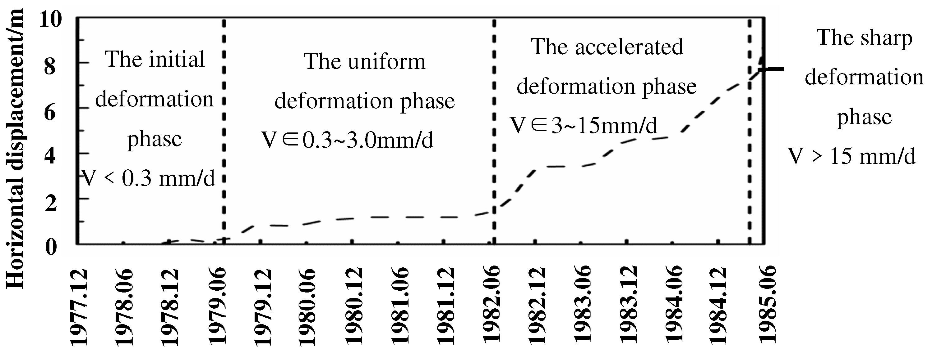
Evaluating the stability of a slope using the strength reduction method requires determining the critical state of the slope, but different criteria may result in varying safety factor calculations. Due to the complexity of analyzing slope stability under earthquake action, a commonly used approach is calculating safety factors based on three criteria and then comprehensively evaluating dynamic stability. Nevertheless, no widely accepted and effective single method for determining seismic slope stability is currently available. Based on the analysis and comparison of relevant research results and the accumulation of long-term work experience, the authors believe that the displacement catastrophe criterion has a clear physical meaning, relatively reliable identification results, and wide application, but there are still applicability problems in specific applications. If the displacement catastrophe point identification method can be improved, its operability and application value in landslide identification will be further improved. Based on the first kind of criteria combined with the evolution law of the actual landslide at different stages, the relative residual displacement increment method is proposed in this paper. As shown in Figure 1, during the development and evolution of the Xintan landslide, according to the cumulative displacement-time curve, it can be divided into four stages: initial deformation, uniform deformation, accelerated deformation, and sharp deformation [37,38]. When the slope is destroyed, it is in the stage of sharp deformation (May to June 1985). Under the action of seismic load, when the slope is unstable, it is in the stage of rapid deformation, and the deformation rate of the landslide mass reaches the maximum value. Therefore, the relative residual displacement increment method (Criterion IV) is proposed to evaluate the seismic stability of the slope. Because the seismic load changes with time, the displacement after the completion of the seismic action can be used as the final displacement of the slope. The curve of the relative displacement-reduction coefficient can be obtained by calculating the relative displacement between the key points inside the landslide mass and the reference points outside the landslide mass. On this basis, the safety factor of the slope is determined by taking the SRF corresponding to the maximum value of the relative residual displacement increment that appears first after a continuous plastic penetration zone.
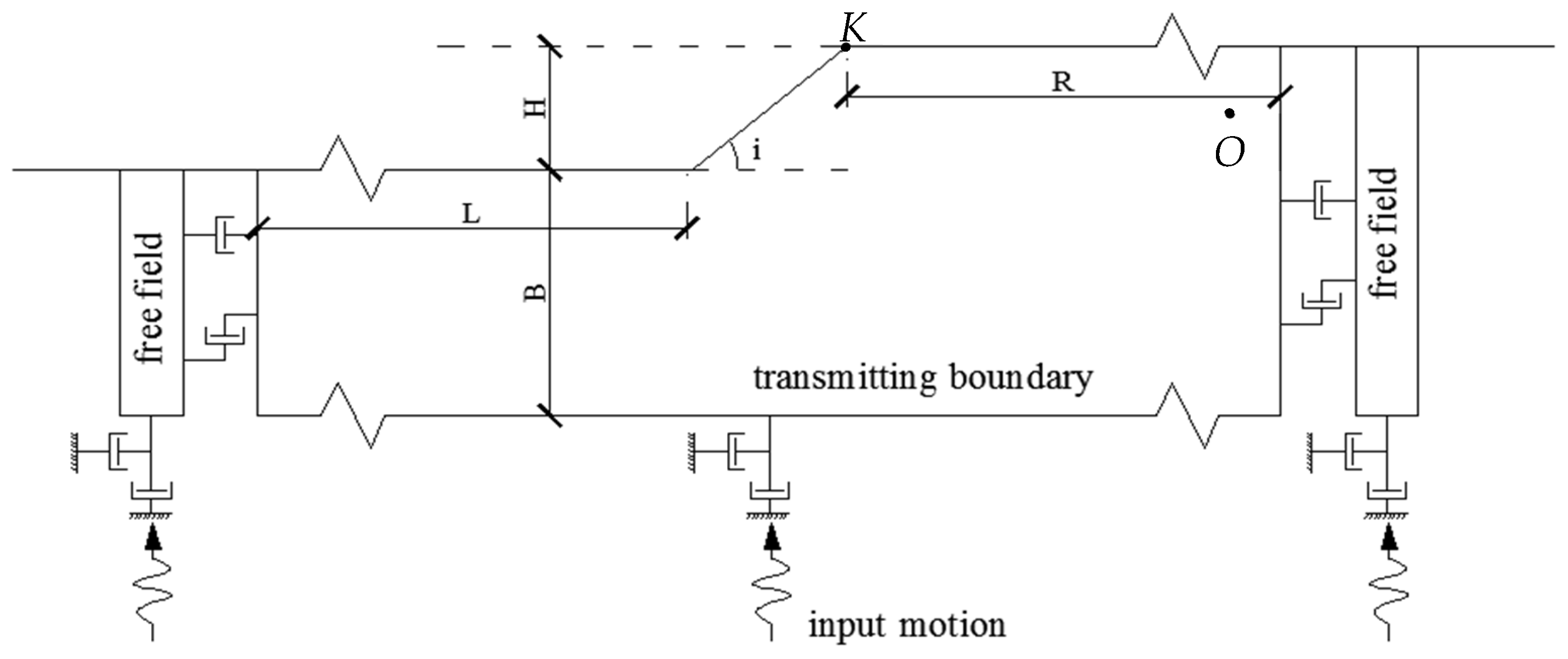
Figure 2 displays the selection of the top point of the landslide body as the key point and the outer point of the landslide body as the reference point . The calculation of the relative displacement of the slope without reduction is as follows:
where represents the displacement of a key point located within the landslide mass, represents the displacement of the reference point located outside the landslide.
The relative residual displacement of the slope after reduction is as follows:
where represents the relative displacement of the slope after the reduction.
The maximum absolute value of the relative residual displacement increment of the slope is as follows:
3. Numerical Analysis
3.1. 2D Slope Model
This paper uses the finite difference software FLAC 7.0 [39] to calculate the slope stability under an earthquake. The slope model is shown in Figure 2. Both sides of the slope model are free boundaries, which can reduce the reflection of the wavelet. The bottom adopts a viscous boundary, which can absorb the energy of the reflected wave.
3.2. Input Ground Motion
Four near-field seismic records are selected as input ground motions for slope dynamic analysis. The seismic records are obtained from the PEER NGA-West2; the detailed information is shown in Table 1. Due to the numerical analysis only considering ground motion frequencies ranging from 0–10 Hz, a low-pass filter with a cutoff frequency of 10 Hz is applied to the acceleration time history. The amplitude of the filtered acceleration is then modulated by 0.1 g. The acceleration time-history curve is shown in Figure 3. Since the bottom boundary is viscous in FLAC, seismic wave input is applied to the bottom boundary in the form of shear stress time history. The finite rigidity of the underlying bedrock is idealized, considering an elastic half-space [40]. The acceleration time history after amplitude modulation is converted into velocity time history v(t), and then the velocity time history is converted into shear stress σs(t). The calculation formula is as follows [41]:
where ρ and vs. represent the medium density and the shear wave velocity, respectively.
3.3. Homogeneous Soil Slope
The homogeneous slope soil mass is an ideal elastic-plastic material conforming to the Mohr–Coulomb yield criterion. The top of the slope is 40 m from the right boundary, the toe of the slope is 40 m from the left boundary, the slope height is 20 m, the slope angle is 45°, and the total thickness of the slope is 40 m. Its material parameters are shown in Table 2 [42].
In the calculation of homogeneous slope, Rayleigh damping is used to simulate the energy dissipation in the dynamic response. The damping matrix C is described as follows [43,44]:
where M and K represent the mass and stiffness matrices, respectively, α and β represent the corresponding scale factor.
According to the suggestion of Kwok et al. [45], two control frequencies are selected respectively: the first-order natural vibration frequency f1 of the slope model and five times the first-order natural vibration frequency (f2 = 5f1). The calculation formulas of α and β are as follows:
where ξ represents the target damping ratio (5%), ω1 and ω2 represent the circular frequency corresponding to f1 and f2, respectively.
In FLAC, the setting of Rayleigh damping needs to input the minimum value of damping ratio ξmin and corresponding frequency fmin, the calculation formula is as follows:
Four seismic waves are input, respectively, and the stability of the homogeneous soil slope under the earthquake action is evaluated by calculating safety factors based on the criterion proposed in this paper and three other types of criteria.
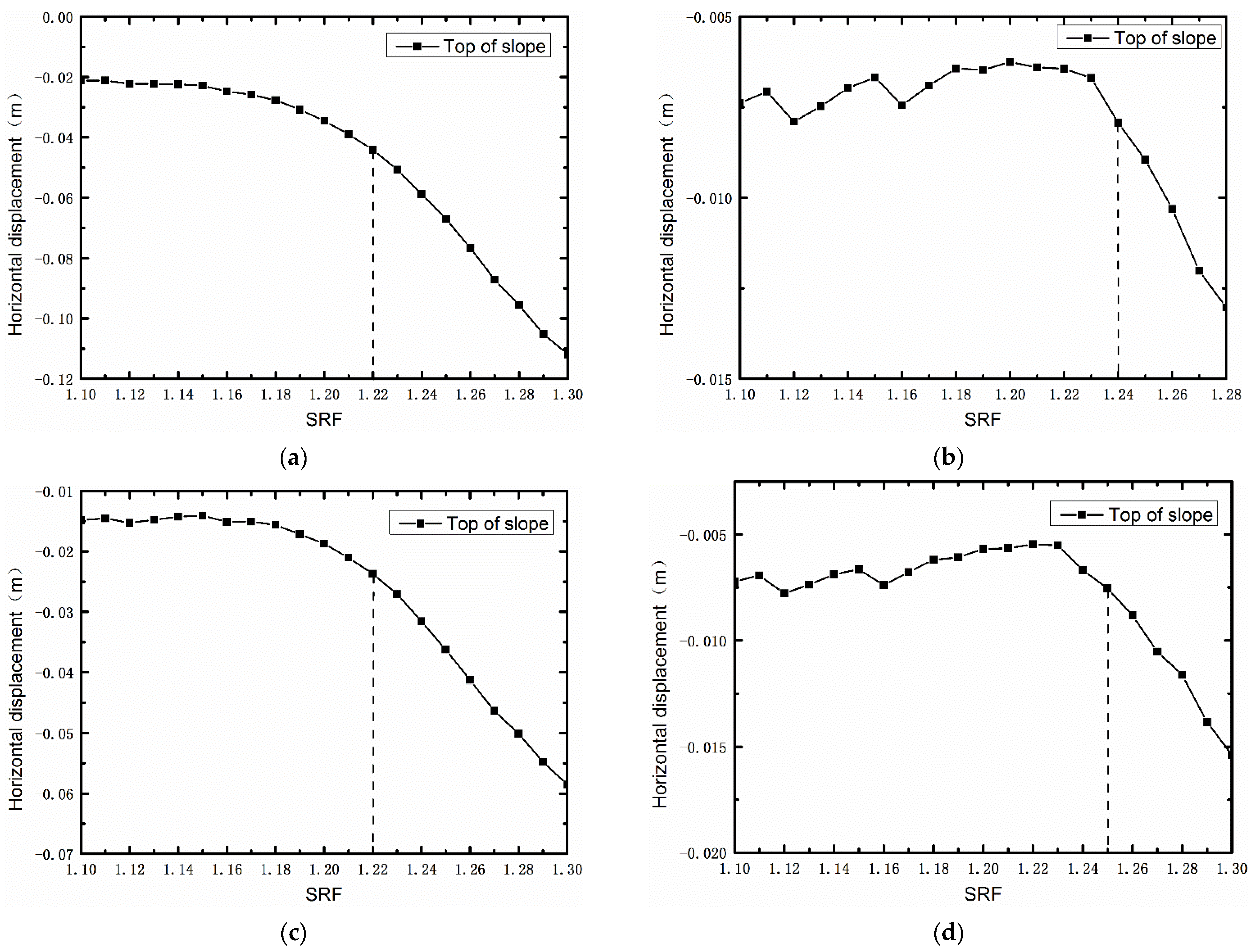
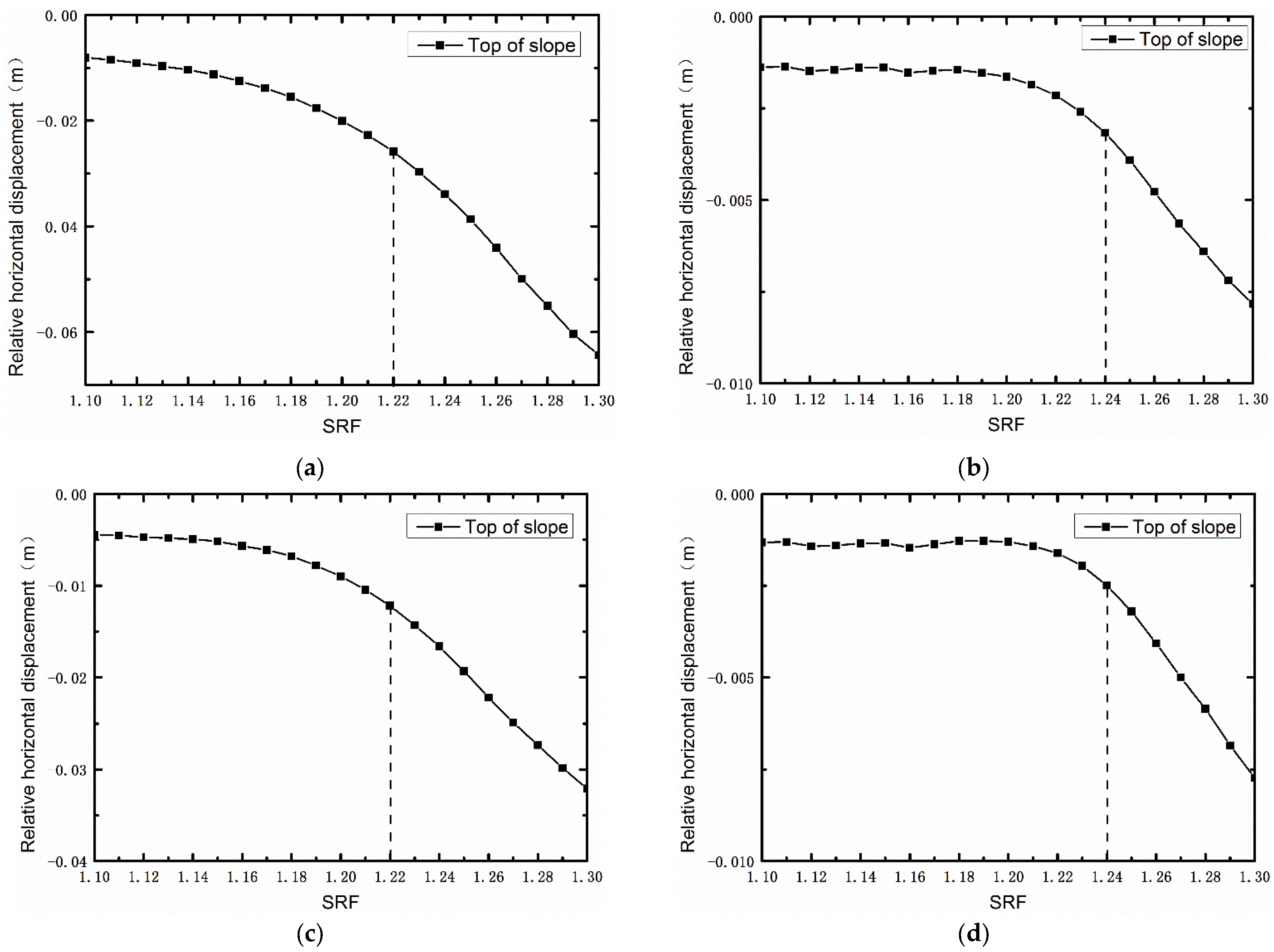
Using the characteristic point displacement catastrophe as the criterion (Criterion I), as depicted in Figure 4 and Figure 5, there are two curves: the vertex displacement-reduction factor curve (Criterion I1) and the relative displacement-reduction factor curve (Criterion I2). In contrast, Figure 4b,d demonstrate that significant fluctuations in the displacement curve can make it challenging to precisely determine the displacement mutation point. To mitigate the impact of curve fluctuation on the reduction factor, the relative displacement curve is used to identify the displacement catastrophe point. Figure 5b,d indicate a reduction in the fluctuation of the relative displacement curve; however, some artificial discrimination errors may still occur.
The penetration zone is taken as the criterion (Criterion II), and the complete penetration zone formed by shear strain increment is taken as the criterion of slope instability. As shown in Figure 6, under this slope model, taking the input Northridge seismic wave as an example, when the reduction factors are 1.24, 1.26, 1.28, and 1.30, the complete through the zone is formed. However, when a continuous plastic penetration zone occurs, the slope does not necessarily break down immediately. Therefore, slope instability cannot be determined by a continuous plastic penetration zone alone.
The iterative non-convergence is used as the criterion (Criterion III), and the criterion for slope instability is based on whether the final displacement diverges after the earthquake. The displacement time history curve is depicted in Figure 7, where Figure 7a,c show that the curve diverges at SRF values of 1.27 and 1.26, respectively. The slope is damaged at this time, leading to a safety factor of 1.26 and 1.25, respectively. In Figure 7b, although the displacement time history curve divergence is indistinguishable, there is a sudden change in displacement. Figure 7d displays a clear displacement time history curve divergence, but its displacement does not change abruptly. Consequently, relying on this criterion to determine slope failure can lead to discrimination errors and failures.
The paper compares and analyzes the advantages and disadvantages of three criteria. Based on the first criterion and taking into account the evolution law of different stages of actual landslides, this paper proposes an improved method for identifying displacement catastrophe points called the relative residual displacement increment method (Criterion IV). The reduction factor corresponding to the maximum value of the relative residual displacement increment for the first time after the sudden change of displacement is the safety factor of the slope. The relative residual displacement increment is shown in Figure 8. Figure 8 shows that after a continuous plastic penetration zone, the SRF corresponding to the maximum relative residual displacement increment for the first time are 1.26, 1.26, 1.25, and 1.26, respectively.
The safety factors of slope under seismic action calculated by different criteria are shown in Table 3. Compared with other criteria, the maximum error between this method and other criteria is 0.033, and the minimum error is only 0.008, indicating that the calculation results of this method agree well with those of other criteria. Thus, this method’s accuracy, applicability, and stability are verified.
3.4. Layered Soil Slope
The layered slope soil mass is an ideal elastic-plastic material conforming to the Mohr–Coulomb yield criterion. The top of the slope is 160 m from the right boundary, the toe of the slope is 160 m from the left boundary, the total length of the slope is 340 m, the slope height is 20 m, the slope angle is 45°, and the total thickness of the slope is 100 m. The slope model is shown in Figure 9, and its material parameters are shown in Table 4.
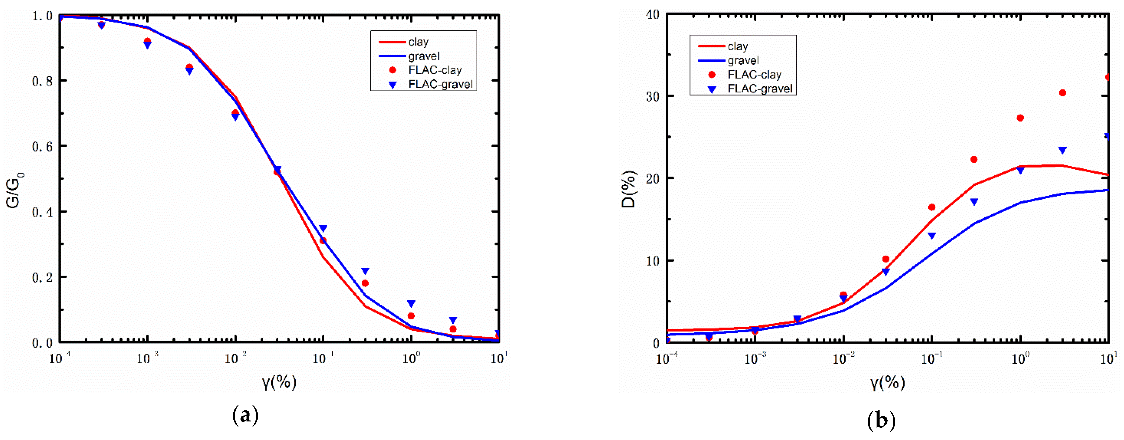
In the seismic calculation of layered slopes, hysteretic damping is used for nonlinear elastoplastic analysis [46]. The G/G0-γc and D-γc curves of two types of soil (Clay soil and gravel soil) in the slope model are shown in Figure 10, respectively. The curve for clay soil (1–3 layers) is calculated according to the empirical model proposed by Darendeli [47]. The G/G0-γc and D-γc relationships of gravel soil (4–5 layers) are based on the empirical curves proposed by Rollins et al. [48]. For the bedrock layer, Rayleigh damping is used.
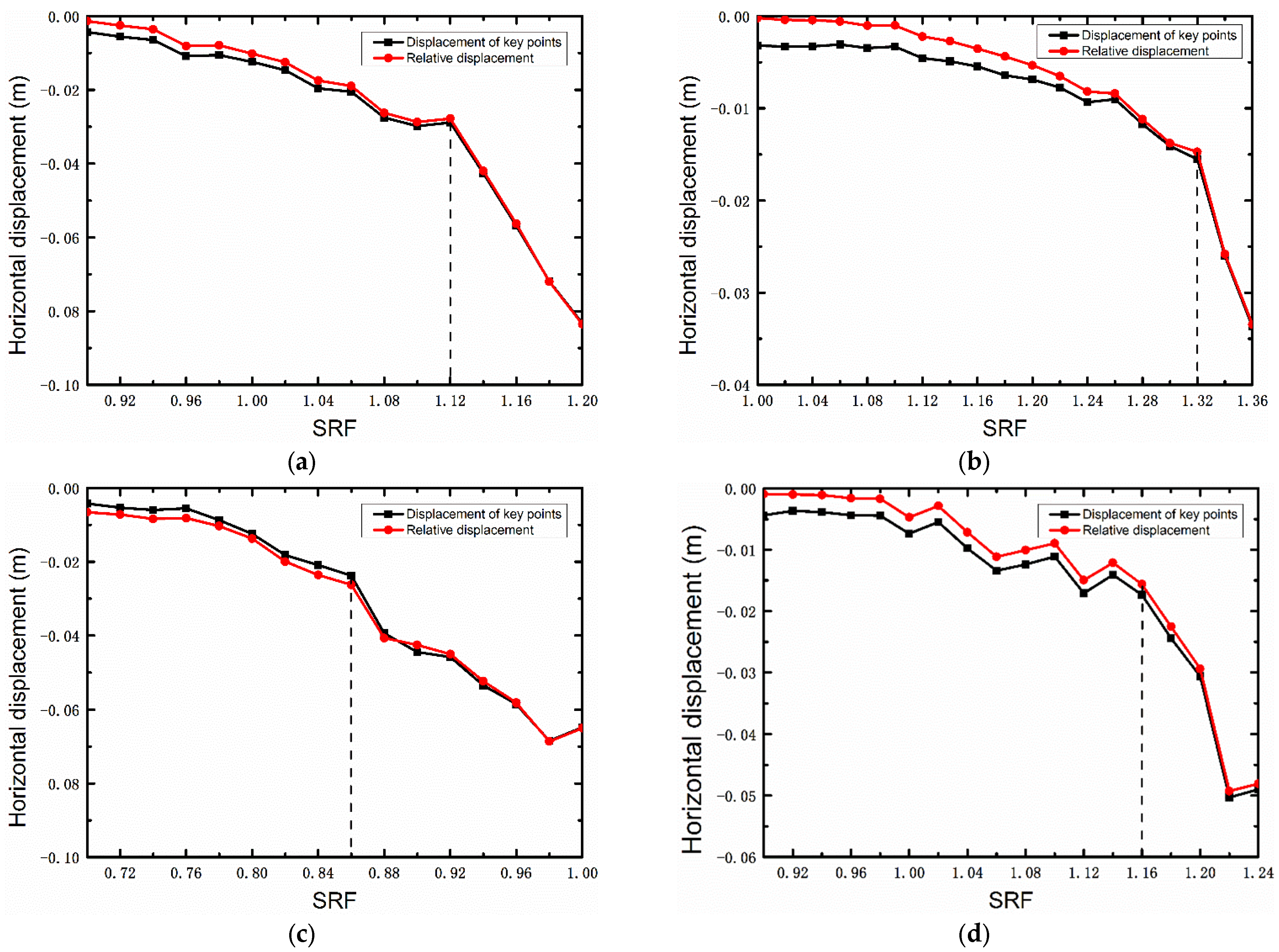
Using the characteristic point displacement catastrophe as the criterion (Criterion I), as depicted in Figure 11, there are two curves: the vertex displacement-reduction factor curve (Criterion I1) and the relative displacement-reduction factor curve (Criterion I2). The displacement curve exhibits significant fluctuations in this example, which can lead to errors when identifying displacement catastrophe points. However, using the maximum value of the relative displacement increment as a criterion can mitigate the impact of these fluctuations and reduce the error.
The penetration zone is taken as the criterion (Criterion II), and the complete penetration zone formed by shear strain increment is taken as the criterion of slope instability. As shown in Figure 12, a complete penetration zone can be formed under this slope model. However, slope instability cannot be determined by a continuous plastic penetration zone alone.
The iterative non-convergence is used as the criterion (Criterion III), and the criterion for slope instability is based on whether the final displacement diverges after the earthquake. The displacement time history curve is shown in Figure 13. After the completion of the earthquake action, its final displacement is in the horizontal state, and the displacement is not obviously divergent. Therefore, slope failure cannot be identified by this criterion.
The maximum value of the relative residual displacement increment is taken as the criterion (Criterion IV) to calculate the safety factor of the slope. The relative residual displacement increment is shown in Figure 14. From Figure 14, it can be seen that after a continuous plastic penetration zone, the SRF corresponding to the maximum relative residual displacement increment for the first time are 1.16, 1.32, 0.92, and 1.20, respectively. The safety factors under seismic action of a slope calculated by different criteria are shown in Table 5. This method’s accuracy, applicability, and stability are once again verified as the maximum error between this method and other criteria is only 0.070, and the minimum error is 0, indicating a high degree of agreement between the present results and those obtained by other criteria.
4. Results and Discussion
This paper employs three types of criteria to compute safety factors for both homogeneous and layered soil slopes when subjected to earthquake action. A comparison and analysis of the benefits and drawbacks of different methods are presented. By conducting a comparative analysis of safety factors, this method’s applicability, accuracy, and stability are verified.
The relative displacement of homogeneous slope changes smoothly with the reduction factor under seismic action, while the change of vertex displacement with the reduction factor fluctuates greatly. Due to the interaction between soil layers, layered soil’s relative displacement and key point displacement have large fluctuations. The safety factors calculated by Criterion I1 and Criterion I2 for homogeneous soil and layered soil are basically the same. Due to the large fluctuation of displacement, Criterion I1 will produce certain judgment errors when judging the sudden change of displacement. Criterion I1 and Criterion I2 can produce a certain degree of human error when judging the displacement catastrophe points. The safety factor of a slope is determined using Criterion II; when a continuous plastic penetration zone occurs, the slope does not necessarily break down immediately. Therefore, slope instability cannot be determined by a continuous plastic penetration zone alone. Criterion III is used to calculate the safety factor of slopes, but it cannot be used for layered soil slopes that exhibit non-divergent displacement after an earthquake. To summarize, obtaining the safety factor of a slope under earthquake action requires considering all three criteria mentioned above.
Based on the first kind of criterion, this paper improves the method of judging the displacement catastrophe points, and the relative residual displacement increment method (Criterion IV) is proposed. The slope safety factors are calculated for homogeneous and layered soil slopes under seismic action. In a homogeneous soil slope, the maximum error between the safety factor calculated by this method and that calculated by other criteria is 0.033, and the minimum error is only 0.008. In layered soil slope, the maximum error between the safety factor calculated by this method and that calculated by other criteria is 0.070, and the minimum error is only 0. Through the seismic calculation of homogeneous and layered soil slopes and the comparison with the other three types of criteria, the applicability, accuracy, and stability of the method in this paper are verified. This article’s method can accurately describe the stress-deformation behavior of slope materials under earthquake action and simulate the damage process of slopes. At the same time, the method in this paper also reflects the influence of different ground motions on slope stability under the same acceleration.
5. Conclusions
The strength reduction dynamic analysis method exhibits great potential for application in the stability analysis of earthquake slopes. This comprehensive dynamic analysis method does not require pre-assumption of the sliding surface, which minimizes the influence of human factors on the safety factor. By utilizing actual seismic waves as input and considering the dynamic interaction between soil masses, the stability of the slope under earthquake action can be directly evaluated. An essential aspect of calculating the earthquake slope safety factor through the strength reduction dynamic analysis method is the reasonable selection of instability criteria. This paper proposes an earthquake slope stability analysis method based on the relative residual displacement increment method. This method combines the first criterion type with the slope’s actual deformation characteristics. By calculating the relative displacement of the key point inside the landslide mass and the reference point outside the landslide mass after each reduction, the safety factor of the slope is determined by calculating the strength reduction factor corresponding to the maximum value of the relative residual displacement increment, which first appears after a continuous plastic penetration zone. We perform earthquake calculations of homogeneous and layered soil slopes and compare our proposed method with three other criteria. Based on the results, we draw the following conclusions:
- (1)
- Criterion I1 considers the sudden change in key point displacement as the instability criterion by comparing and analyzing three different criteria. When the seismic force acts, the displacement of key points fluctuates significantly, which can interfere with the identification of displacement catastrophe points. Using the sudden change in relative displacement as a criterion (Criterion I2) can somewhat reduce the interference caused by displacement fluctuations. However, Criterion I2 may still lead to some human error when identifying displacement catastrophe points. While Criteria II and III can be used to assess slope instability, they may not provide the slope safety factor in some cases. Therefore, a comprehensive consideration of all three criteria is necessary to obtain an accurate safety factor for earthquake slope stability calculations;
- (2)
- By comparing and analyzing this method with three other criteria, the strength reduction factor corresponding to the maximum value of the relative residual displacement increment, which appears after an abrupt change in displacement, is used as the safety factor for the slope. This improves the method of identifying displacement catastrophe points, avoids errors caused by displacement fluctuations, and reduces human error in judging displacement catastrophe points. As a result, the displacement catastrophe criterion’s accuracy, stability, and applicability are enhanced.
Author Contributions
Conceptualization, W.S.; Methodology, W.S.; Formal analysis, W.S.; Investigation, J.M.; Writing—original draft, W.S.; Writing—review & editing, G.W.; Supervision, G.W. All authors have read and agreed to the published version of the manuscript.
Funding
This research was sponsored by the National Key R&D Program of China (Grant No. 2018YFD1100405).
Data Availability Statement
The original contributions presented in the study are included in the article, further inquiries can be directed to the corresponding authors.
Conflicts of Interest
The authors declare no conflicts of interest.
References
- Wu, M.T.; Liu, F.C.; Yang, J. Seismic response of stratified rock slopes due to incident P and SV waves using a semi-analytical approach. Eng. Geol. 2022, prepublish. [Google Scholar] [CrossRef]
- Yin, Y.P.; Wang, F.W.; Sun, P. Landslide hazards triggered by the 2008 Wenchuan earthquake, Sichuan, China. Landslides 2009, 6, 139–151. [Google Scholar] [CrossRef]
- Tang, C.; Zhu, J.; Qi, X.; Ding, J. Landslides induced by the Wenchuan earthquake and the subsequent strong rainfall event: A case study in the Beichuan area of China. Eng. Geol. 2011, 122, 22–23. [Google Scholar] [CrossRef]
- Li, S.; Kang, L.M.; Yu, B.; Li, J.; Feng, L.; Zhang, S.; Zhu, W.; Yao, X. Dynamic reliability analysis of bedding rock slopes under earthquake actions. Build. Struct. 2021, 51, 1679–1683. (In Chinese) [Google Scholar]
- Jibson, R.W. Methods for assessing the stability of slopes during earthquakes—A retrospective. Eng. Geol. 2011, 122, 43–50. [Google Scholar] [CrossRef]
- Terzhagi, K. Mechanism of Landslides Application of Geology to Engineering Practice (Berkey Volume); Geological Society of America: New York, NY, USA, 1950. [Google Scholar] [CrossRef]
- Newmark, N.M. Effects of earthquakes on dams and embankments. Geotechnique 1965, 15, 139–160. [Google Scholar] [CrossRef]
- Clough, R.W.; Chopra, A.K. Earthquake stress analysis in earth dams. ASCE J. Eng. Mech. Div. 1966, 92, 197–211. [Google Scholar] [CrossRef]
- Groumpos, P.P. A Critical Historic Overview of Artificial Intelligence: Issues, Challenges, Opportunities, and Threats. Artif. Intell. Appl. 2023, 1, 197–213. [Google Scholar] [CrossRef]
- Alkhaled, L.; Khamis, T. Supportive Environment for Better Data Management Stage in the Cycle of ML Process. Artif. Intell. Appl. 2023, 2, 1–8. [Google Scholar] [CrossRef]
- Bui, D.T.; Moayedi, H.; Gör, M.; Jaafari, A.; Foong, L.K. Predicting slope stability failure through machine learning paradigms. ISPRS Int. J. Geo-Inf. 2019, 8, 395. [Google Scholar] [CrossRef]
- Gheisari, M.; Ebrahimzadeh, F.; Rahimi, M.; Moazzamigodarzi, M.; Liu, Y.; Pramanik, P.K.D.; Heravi, M.A.; Mehbodniya, A.; Ghaderzadeh, M.; Feylizadeh, M.R.; et al. Deep learning: Applications, architectures, models, tools, and frameworks: A comprehensive survey. CAAI Trans. Intell. Technol. 2023, 8, 581–606. [Google Scholar] [CrossRef]
- Fan, Q.Q.; Jiang, M.; Huang, W.T.; Jiang, Q. Considering spatiotemporal evolutionary information in dynamic multi-objective optimisation. CAAI Trans. Intell. Technol. 2023, 1–21. [Google Scholar] [CrossRef]
- Leshchinsky, D.; San, K.C. Pseudo-static seismic stability of slopes: Design charts. J. Geotech. Eng. 1994, 120, 1514–1532. [Google Scholar] [CrossRef]
- Ausilio, E.; Conte, E.; Dente, G. Seismic stability analysis of reinforced slopes. Soil Dyn. Earthq. Eng. 2000, 19, 159–172. [Google Scholar] [CrossRef]
- Luan, M.T.; Li, Z.; Fan, Q.L. Analysis and evaluation of pseudo-static seismic stability and seism-induced sliding movement of earth-rock dams. Rock Soil Mech. 2007, 28, 224–230. (In Chinese) [Google Scholar]
- Zhao, L.H.; Li, L.; Yang, F.; Dan, H.C.; Liu, X. Dynamic stability pseudo-static analysis of reinforcement soil slopes. Chin. J. Rock Mech. Eng. 2009, 28, 1904–1917. (In Chinese) [Google Scholar]
- Deng, D.P.; Li, L. Pseudo-static stability analysis of slope under earthquake based on a new method of searching for sliding surface. Chin. J. Rock Mech. Eng. 2012, 31, 86–98. (In Chinese) [Google Scholar]
- Qin, C.B.; Chian, S.C. Kinematic analysis of seismic slope stability with a discretisation technique and pseudo-dynamic approach: A new perspective. Geotechnique 2018, 68, 492–503. [Google Scholar] [CrossRef]
- Courant, R. Variational methods for the solution of problems of equilibrium and vibrations. Bull. Am. Math. Soc. 1943, 49, 1–23. [Google Scholar] [CrossRef]
- Clough, R.W. The finite element method in plane stress analysis. In Proceedings of the 2nd Conference on Electronic Computation, Pittsburgh, PA, USA, 8–9 September 1960; American Society of Civil Engineers, Structural Division: Pittsburgh, PA, USA, 1960. [Google Scholar]
- Seed, H.B.; Lee, K.L.; Idriss, I.M.; Makdisi, F. Analysis of the Slides in the San Fernando Dams during the Earthquake of Feb. 9, 1971; Report No. EERC 73-2; University of California: Berkeley, CA, USA, 1973. [Google Scholar] [CrossRef]
- Prevost, J.H. DYNAFLOW: A Nonlinear Transient Finite Element Analysis Program; Technical Report; Department of Civil Engineering and Operations Research, Princeton University: Princeton, NJ, USA, 1981. [Google Scholar]
- Griffiths, D.V.; Prevost, J.H. Two- and three-dimensional dynamic finite element analyses of the Long Valley Dam. Geotechnique 1988, 38, 367–388. [Google Scholar] [CrossRef]
- Elgamal, A.M.; Scott, R.F.; Succarieh, M.F.; Yan, L. La Villita dam response during five earthquakes including permanent deformation. J. Geotech. Eng. 1990, 116, 1443–1462. [Google Scholar] [CrossRef]
- Zhou, J.W.; Cui, P.; Yang, X.G. Dynamic process analysis for the initiation and movement of the Donghekou landslide-debris flow triggered by the Wenchuan earthquake. J. Asian Earth Sci. 2013, 76, 70–84. [Google Scholar] [CrossRef]
- Luo, J.; Pei, X.J.; Evans, S.G.; Huang, R. Mechanics of the earthquake induced Hongshiyan landslide in the 2014 Mw 6.2 Ludian earthquake, Yunnan, China. Eng. Geol. 2019, 251, 197–213. [Google Scholar] [CrossRef]
- Dawson, E.M.; Roth, W.H.; Drescher, A. Slope stability analysis by strength reduction. Geotechnique 1999, 49, 835–840. [Google Scholar] [CrossRef]
- Zheng, Y.R.; Zhao, S.Y.; Zheng, L.Y. Slope stability analysis by strength reduction FEM. Eng. Sci. 2002, 4, 57–61+78. (In Chinese) [Google Scholar]
- Dai, M.L.; Li, T.C. Analysis of dynamic stability safety evaluation for complex rock slope by strength reduction numerical method. Chin. J. Rock Mech. Eng. 2007, 192, 2749–2754. (In Chinese) [Google Scholar]
- Liu, K.Q.; Liu, H.Y. Stability Analysis of Soil-rock Mixture Slope under Earthquake. J. Disaster Prev. Mitig. Eng. 2022, 42, 224–230. [Google Scholar] [CrossRef]
- Li, D.J.; Zhang, J.Y.; Lian, Y.W.; Tang, W. Dynamic Stability Analysis of Slope Under the Impact Load of Large Diameter Punched Cast-in-Place Pile. Int. J. Geosynth. Ground Eng. 2023, 9, 29. [Google Scholar] [CrossRef]
- Ge, X.R.; Ren, J.X.; Li, C.G.; Zheng, H. 3D-FE analysis of deep sliding stability of #3 dam foundation of left power house of the Three Gorges Project. Chin. J. Geotech. Eng. 2003, 25, 389–394. (In Chinese) [Google Scholar]
- Zheng, Y.R.; Ye, H.L.; Huang, R.Q. Analysis and discussion of failure mechanism and fracture surface of slope under earthquake. Chin. J. Rock Mech. Eng. 2009, 28, 1714–1723. (In Chinese) [Google Scholar]
- Li, H.B.; Xiao, K.Q.; Liu, Y.Q. Factor of safety analysis of bedding rock slope under seismic load. Chin. J. Rock Mech. Eng. 2007, 191, 2385–2394. (In Chinese) [Google Scholar]
- Wu, X.Y.; Liu, Q.; Cang, J.Y. The Sensitivity and Reliability Analysis of Slope Stability Based on Strength Reduction FEM. Appl. Mech. Mater. 2013, 353–356, 491–494. [Google Scholar] [CrossRef]
- Li, C.; Zhu, J.B.; Wang, B.; Jiang, Y.; Liu, X.; Zeng, P. Critical deformation velocity of landslides in different deformation phases. Chin. J. Rock Mech. Eng. 2016, 35, 1407–1414. (In Chinese) [Google Scholar]
- Sun, W.J.; Wang, G.X.; Zhang, L.L. Slope stability analysis by strength reduction method based on average residual displacement increment criterion. Bull. Eng. Geol. Environ. 2021, 80, 4367–4378. [Google Scholar] [CrossRef]
- Itasca Consulting Group Inc. Itasca FLAC 7.0: Fast Lagrangian Analysis of Continua. User’s Guide; Itasca Consulting Group Inc.: Minneapolis, MN, USA, 2011; Available online: www.itascacg.com (accessed on 12 March 2024).
- Karafagka, S.; Fotopoulou, S.; Karatzetzou, A.; Kroupi, G.; Pitilakis, K. Seismic performance and vulnerability of gravity quay wall in sites susceptible to liquefaction. Acta Geotech. 2023, 18, 2733–2754. [Google Scholar] [CrossRef]
- Joyner, W.B.; Chen, A.T.F. Calculation of nonlinear ground response in earthquakes. Bull. Seismol. Soc. Am. 1975, 65, 1315–1336. [Google Scholar] [CrossRef]
- Li, J. Study on Determination and Application of Slope Safety Factor under Seismic Action. Master’s Thesis, Chongqing Jiaotong University, Chongqing, China, 2011. (In Chinese). [Google Scholar]
- Bouckovalas, G.D.; Papadimitriou, A.G. Numerical evaluation of slope topography effects on seismic ground motion. Soil Dyn. Earthq. Eng. 2005, 25, 547–558. [Google Scholar] [CrossRef]
- Zhang, Z.Z.; Fleurisson, J.A.; Pellet, F. The effects of slope topography on acceleration amplification and interaction between slope topography and seismic input motion. Soil Dyn. Earthq. Eng. 2018, 113, 420–431. [Google Scholar] [CrossRef]
- Kwok, A.O.L.; Stewart, J.P.; Hashash, Y.M.A.; Matasovic, N.; Pyke, R.; Wang, Z.; Yang, Z. Use of exact solutions of wave propagation problems to guide lmplementation of Nonlinear seismic ground response analysis procedures. J. Geotech. Geoenviron. Eng. 2007, 133, 1385–1398. [Google Scholar] [CrossRef]
- Ding, Y.; Wang, G.X.; Yang, F.J. Parametric investigation on the effect of near-surface soil properties on the topographic amplification of ground motions. Eng. Geol. 2020, 273, 105687. [Google Scholar] [CrossRef]
- Darendeli, M.B. Development of a New Family of Normalized Modulus Reduction and Material Damping Curves; University of Texas at Austin: Austin, TX, USA, 2001. [Google Scholar]
- Rollins, K.M.; Evans, M.D.; Diehl, N.B.; William, D.D., III. Shear modulus and damping relationships for gravels. J. Geotech. Geoenviron. Eng. 1998, 124, 396–405. [Google Scholar] [CrossRef]
Figure 1.
The displacement-time curve of the Xintan landslide.

Figure 2.
Schematic view of the 2D slope model.

Figure 3.
Acceleration time histories of the input motions.

Figure 4.
The displacement-SRF curves. (a) Northridge (SRF = 1.22), (b) San Francisco (SRF = 1.24), (c) Whittier Narrows (SRF = 1.22), (d) Whittier Narrows-1 (SRF = 1.25).
Figure 4.
The displacement-SRF curves. (a) Northridge (SRF = 1.22), (b) San Francisco (SRF = 1.24), (c) Whittier Narrows (SRF = 1.22), (d) Whittier Narrows-1 (SRF = 1.25).

Figure 5.
The relative displacement-SRF curves. (a) Northridge (SRF = 1.22), (b) San Francisco (SRF = 1.24), (c) Whittier Narrows (SRF = 1.22), (d) Whittier Narrows-1 (SRF = 1.24).
Figure 5.
The relative displacement-SRF curves. (a) Northridge (SRF = 1.22), (b) San Francisco (SRF = 1.24), (c) Whittier Narrows (SRF = 1.22), (d) Whittier Narrows-1 (SRF = 1.24).

Figure 6.
Shear strain increment penetration zone (Northridge) (m). (a) SRF = 1.24, (b) SRF = 1.26, (c) SRF = 1.28, (d) SRF = 1.30.
Figure 6.
Shear strain increment penetration zone (Northridge) (m). (a) SRF = 1.24, (b) SRF = 1.26, (c) SRF = 1.28, (d) SRF = 1.30.

Figure 7.
Displacement non-convergence. (a) Northridge (SRF = 1.26), (b) San Francisco, (c) Whittier Narrows (SRF = 1.25), (d) Whittier Narrows-1.
Figure 7.
Displacement non-convergence. (a) Northridge (SRF = 1.26), (b) San Francisco, (c) Whittier Narrows (SRF = 1.25), (d) Whittier Narrows-1.

Figure 8.
Relative residual displacement increment and strength reduction factor histogram. (a) Northridge (SRF = 1.26), (b) San Francisco (SRF = 1.26), (c) Whittier Narrows (SRF = 1.25), (d) Whittier Narrows-1 (SRF = 1.26).
Figure 8.
Relative residual displacement increment and strength reduction factor histogram. (a) Northridge (SRF = 1.26), (b) San Francisco (SRF = 1.26), (c) Whittier Narrows (SRF = 1.25), (d) Whittier Narrows-1 (SRF = 1.26).

Figure 9.
Distribution of shear-wave velocity in the 2D slope model (m/s).

Figure 10.
Normalized (a) shear modulus (G/G0-γ) and (b) damping ratio (D-γ) curves for all the soil types used in the numerical analysis. The corresponding relationships obtained using hysteretic damping in FLAC are also shown.
Figure 10.
Normalized (a) shear modulus (G/G0-γ) and (b) damping ratio (D-γ) curves for all the soil types used in the numerical analysis. The corresponding relationships obtained using hysteretic damping in FLAC are also shown.

Figure 11.
The displacement-SRF curves. (a) Northridge (SRF = 1.12), (b) San Francisco (SRF = 1.32), (c) Whittier Narrows (SRF = 0.86), (d) Whittier Narrows-1 (SRF = 1.16).
Figure 11.
The displacement-SRF curves. (a) Northridge (SRF = 1.12), (b) San Francisco (SRF = 1.32), (c) Whittier Narrows (SRF = 0.86), (d) Whittier Narrows-1 (SRF = 1.16).

Figure 12.
Shear strain increment penetration zone (m). (a) Northridge (SRF = 1.14), (b) San Francisco (SRF = 1.34), (c) Whittier Narrows (SRF = 0.94), (d) Whittier Narrows-1 (SRF = 1.20).
Figure 12.
Shear strain increment penetration zone (m). (a) Northridge (SRF = 1.14), (b) San Francisco (SRF = 1.34), (c) Whittier Narrows (SRF = 0.94), (d) Whittier Narrows-1 (SRF = 1.20).

Figure 13.
Displacement non-convergence. (a) Northridge, (b) San Francisco, (c) Whittier Narrows, (d) Whittier Narrows-1.
Figure 13.
Displacement non-convergence. (a) Northridge, (b) San Francisco, (c) Whittier Narrows, (d) Whittier Narrows-1.

Figure 14.
Relative residual displacement increment and strength reduction factor histogram. (a) Northridge (SRF = 1.16), (b) San Francisco (SRF = 1.32), (c) Whittier Narrows (SRF = 0.92), (d) Whittier Narrows-1 (SRF = 1.20).
Figure 14.
Relative residual displacement increment and strength reduction factor histogram. (a) Northridge (SRF = 1.16), (b) San Francisco (SRF = 1.32), (c) Whittier Narrows (SRF = 0.92), (d) Whittier Narrows-1 (SRF = 1.20).


Table 1.
Information of the selected seismic records.
| No. | Earthquake | Date | MW | Rjb (km) | Station | VS30 (m/s) |
|---|---|---|---|---|---|---|
| 1 | Northridge | 17 January 1994 | 6.7 | 23.1 | Vasquez Rocks Park | 996.4 |
| 2 | San Francisco | 22 March 1957 | 5.3 | 9.74 | Golden Gate Park | 874.72 |
| 3 | Whittier Narrows | 1 October 1987 | 6 | 6.78 | Pasadena—CIT Kresge Lab | 969.1 |
| 4 | Whittier Narrows-1 | 1 October 1987 | 6 | 47.25 | Vasquez Rocks Park | 996.4 |
Table 2.
Material parameters.
| c (KPa) | ψ (°) | γ (kN/m3) | G (MPa) | K (MPa) | Rm (MPa) |
|---|---|---|---|---|---|
| 40 | 30 | 22 | 30 | 60 | 0.004 |
Where c is the effective cohesion, ψ is the effective friction angle, γ is the bulk density, G is the shear modulus, K is the bulk modulus, Rm is the tensile strength.
Table 3.
Safety factor of homogeneous slopes calculated by different criteria under seismic action.
| Slope Failure Criteria | Safety Factors under Different Earthquakes | |||
|---|---|---|---|---|
| Northridge | San Francisco | Whittier Narrows | Whittier Narrows-1 | |
| Criterion I1 | 1.22 | 1.24 | 1.22 | 1.25 |
| Criterion I2 | 1.22 | 1.24 | 1.22 | 1.24 |
| Criterion II | 1.23 | 1.24 | 1.23 | 1.24 |
| Criterion III | 1.27 | - | 1.26 | - |
| Criterion IV | 1.26 | 1.26 | 1.25 | 1.26 |
| Error((IV − I1)/I1) | 0.033 | 0.016 | 0.025 | 0.008 |
| Error((IV − I2)/I2) | 0.033 | 0.016 | 0.025 | 0.016 |
| Error((IV − II)/II) | 0.024 | 0.016 | 0.016 | 0.016 |
| Error((IV − III)/III) | −0.008 | - | −0.008 | - |
Table 4.
Material parameters.
| No. | Material | Thickness (m) | VS (m/s) | γ (kN/m3) | ν | Constitutive Law | ψ (°) | c (KPa) |
|---|---|---|---|---|---|---|---|---|
| 1 | Silty clay | 3 | 176.8 | 18.7 | 0.3 | Mohr–Coulomb | 25 | 35 |
| 2 | clay | 8 | 220.3 | 20 | 0.3 | Mohr–Coulomb | 25 | 40 |
| 3 | clay | 6 | 326.6 | 21 | 0.3 | Mohr–Coulomb | 30 | 42 |
| 4 | Clayey sandy gravel | 10 | 512.2 | 21.6 | 0.3 | Mohr–Coulomb | 31 | 30 |
| 5 | Clayey sandy gravel | 20 | 693.1 | 22 | 0.3 | Mohr–Coulomb | 31 | 20 |
| 6 | Bedrock | 53 | 774.2 | 22 | 0.3 | Elastic |
Table 5.
Safety factor of layered soil slopes calculated by different criteria under seismic action.
Table 5.
Safety factor of layered soil slopes calculated by different criteria under seismic action.
| Slope Failure Criteria | Safety Factors under Different Earthquakes | |||
|---|---|---|---|---|
| Northridge | San Francisco | Whittier Narrows | Whittier Narrows-1 | |
| Criterion I 1 | 1.12 | 1.32 | 0.86 | 1.16 |
| Criterion I 2 | 1.12 | 1.32 | 0.86 | 1.16 |
| Criterion II | 1.12 | 1.32 | 0.92 | 1.18 |
| Criterion III | - | |||
| Criterion IV | 1.16 | 1.32 | 0.92 | 1.20 |
| Error((IV − I1)/I1) | 0.036 | 0.000 | 0.070 | 0.034 |
| Error((IV − I2)/I2) | 0.036 | 0.000 | 0.070 | 0.034 |
| Error((IV − II)/II) | 0.036 | 0.000 | 0.000 | 0.017 |
| Error((IV − III)/III) | - | |||
Disclaimer/Publisher’s Note: The statements, opinions and data contained in all publications are solely those of the individual author(s) and contributor(s) and not of MDPI and/or the editor(s). MDPI and/or the editor(s) disclaim responsibility for any injury to people or property resulting from any ideas, methods, instructions or products referred to in the content. |
© 2024 by the authors. Licensee MDPI, Basel, Switzerland. This article is an open access article distributed under the terms and conditions of the Creative Commons Attribution (CC BY) license (https://creativecommons.org/licenses/by/4.0/).
Share and Cite
MDPI and ACS Style
Sun, W.; Wang, G.; Ma, J. Stability Analysis of Seismic Slope Based on Relative Residual Displacement Increment Method. Buildings 2024, 14, 1211. https://0-doi-org.brum.beds.ac.uk/10.3390/buildings14051211
AMA Style
Sun W, Wang G, Ma J. Stability Analysis of Seismic Slope Based on Relative Residual Displacement Increment Method. Buildings. 2024; 14(5):1211. https://0-doi-org.brum.beds.ac.uk/10.3390/buildings14051211
Chicago/Turabian StyleSun, Weijian, Guoxin Wang, and Juntao Ma. 2024. "Stability Analysis of Seismic Slope Based on Relative Residual Displacement Increment Method" Buildings 14, no. 5: 1211. https://0-doi-org.brum.beds.ac.uk/10.3390/buildings14051211
Note that from the first issue of 2016, this journal uses article numbers instead of page numbers. See further details here.