1. Introduction: Electrical Bearing Currents and Bearing Surface Damage
Inverter-driven variable-speed AC electrical machines, mainly three-phase synchronous or induction machines, are used in many industrial applications–in electric and hybrid cars, trains, street cars, ships, aircrafts, household appliances etc.–at different power and speed levels. Fast-switching power electronic devices, based on Silicon or Silicon-Carbide-semiconductor transistors, supply the torque-generating currents to the machine’s three-phase stator windings with a fundamental frequency typically up to 1 kHz. In addition, a fluctuating electrical potential of the stator winding with respect to the electrically grounded base of the electrical machine occurs with the switching frequency, typically at several kHz, called common mode (CM) voltage [
1]. This CM voltage causes parasitic high-frequency (HF) currents of small amplitude from the motor electrical terminals to the electric ground of the drive system [
2], which flow through the conductive and capacitive motor components, e.g., motor bearings [
3,
4]. These currents may also indirectly induce a current flow in the bearings magnetically. These HF bearing currents may cause a corrugation of the bearing raceway surface, causing increased audible noise and motor vibrations, a deterioration of the bearing lubricant, increased bearing friction losses and bearing heating, and, in the worst-case, a bearing failure [
5,
6,
7], e.g., via a cage mechanical break. Different bearing current effects are described in the literature, e.g., [
8].
First, with fully lubricated bearings, apart from harmless capacitive HF currents via the electrically insulating lubrication film (e.g., film thickness
h = 0.2 μm), considerable discharge currents may occur in the lubrication film [
9] if the electrical voltage at the lubricant film surpasses its breakdown voltage (e.g.,
U = 6 V). The corresponding electrical field strength
E =
U/
h (e.g., 30 kV/mm) is ionizing the lubricant molecules [
10,
11,
12,
13,
14], leading to short sparks of durations typically around 1 μs. The resulting EDM bearing current (EDM: Electric Discharge Machining [
1]) oscillates due to the inductive and capacitive machine components in the MHz-range. These electric currents discharge the parasitic capacitances of the electrical machine [
1,
15]. The endangerment of the bearing currents is assessed with “apparent” bearing current densities
J =
I/
AHz, where
I is the amplitude of the current and
AHz is the bearing
Hertz’ian area [
1]. If
J < 0.3 A/mm
2, the corresponding craters, with diameters of typically around 1 μm on the bearing raceway surface, are sufficiently flattened by the roller elements [
1,
16]. If
J > 0.3 A/mm
2, for EDM bearing currents, the exposed surface shows a grey trace (called “grey frosting” [
2,
15]), which may still allow a further bearing operation [
17].
Second, the HF CM winding-stator currents excite an additional HF magnetic field inside the machine, which, due to
Faraday’s law, induces a voltage on a loop path, composing both bearings, rotor shaft, and stator iron parts, resulting in so-called circular bearing currents [
1]. These currents occur at both low and medium speeds in AC machines of frame sizes ca. above 200 mm [
1,
15]. Compared to the EDM bearing currents, the circular bearing currents happen more frequently, have longer durations, higher amplitudes, and lower frequencies, and are more dangerous for the bearings [
15]. Similar to the circular bearing currents, rotor-to-ground bearing currents may endanger the bearings, even in machines with smaller frame sizes below 200 mm, when the rotor is electrically connected to the ground with a low HF impedance, e.g., via a gear box or a milling device [
1]. Any bearing current between the ball and the raceway is limited through the so-called
a-spots, due to the lubrication film and the covering oxide layer. The very high local current densities at the a-spots result in very high local temperatures. These temperatures degrade the lubricant by molecule dissociation, release carbon, thus blackening the oil and reducing the lubrication effect. The effect of the bearing current flow may gradually develop into the fluting pattern [
1,
18,
19].
The cause-and-effect chain of the generation of the fluting pattern has been under investigation for a long time [
3,
4,
5,
6,
7,
8,
18,
19,
20,
21]. A theoretically established detailed physical model, proven by simulation, is currently missing. The following mechanism is obviously involved. Due the surface roughness, the real mechanical contact area between the ball and raceway is smaller than the calculated
Hertz’ian area
A [
22]. The elastic and plastic deformations of the asperity peaks within the
Hertz’ian area [
23] provide the real mechanical contact area. The increased surface roughness due the current flow leads to micro-Elasto-Hydrodynamic Lubrication (micro-EHL), where the oil is pressed into the surface valleys [
24]. Thus, for a rough surface, asperity peaks may still have electrical contacts (
a-spots) [
25], even when bearing parts are dominantly separated via a lubrication film [
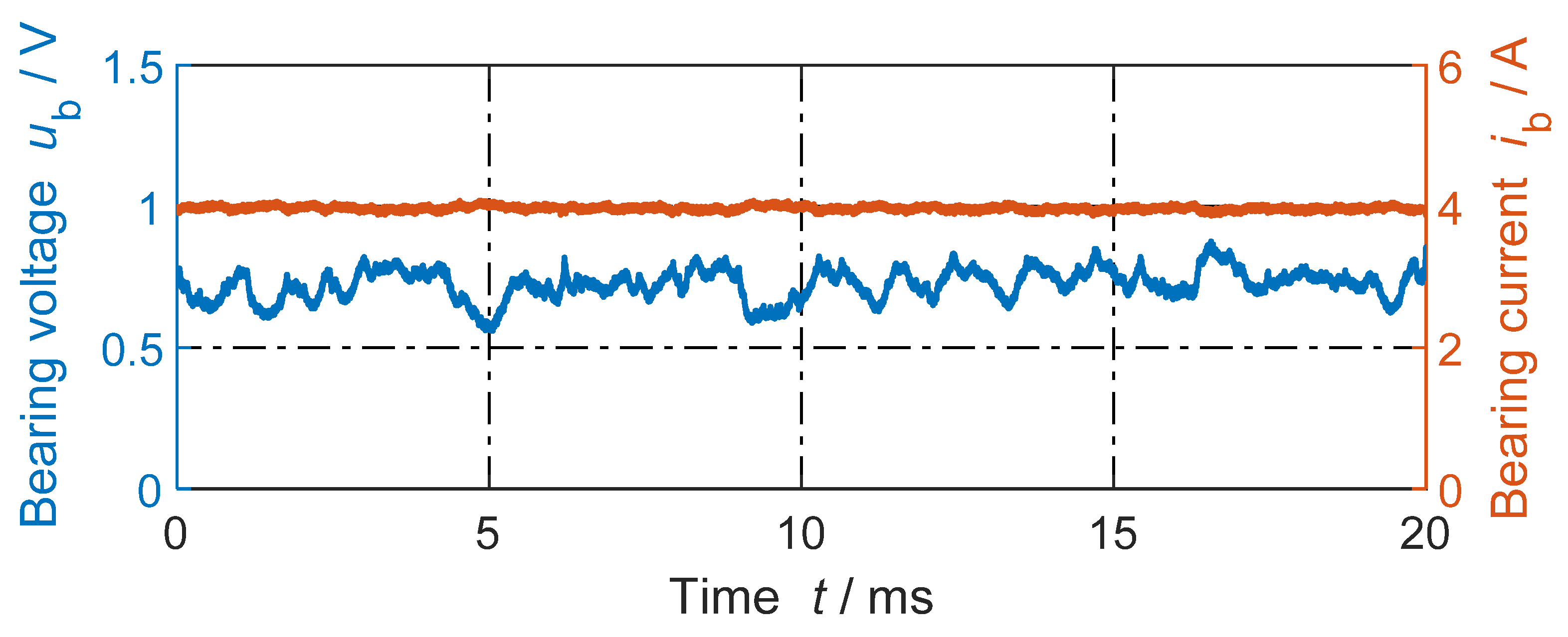
26]. At DC bearing currents, the bearing voltage drop between inner and outer bearing rings remains constant around 1 V, independent of the amplitude of bearing current [
27]. This voltage is sufficient to cause very high local contact temperatures above 1000 °C on moving contact partners in a very short time (below 1 μs). This leads to melting of the micro-size volume of the
a-spot with a typical radius of 1 μs [
25], allowing the current flow. Similar local temperatures occur at inverter-fed motors at impulse bearing current flow. Catalytic effects of the metal-oxide debris promote the oxidation process in the lubricant [
28] and lead to an increased lubricant conductivity. Due to this current flow, a build-up of an oxide layer on the bearing raceway surface occurs [
20]. In electrical steel contacts, it is well established that the oxide surface layers are formed due to the sliding of the asperities, causing a significant amount of Fe
2+ and Fe
3+ compared to the bulk steel [
29,
30]. These oxides form an insulating layer between two mechanically touching bodies, constraining the current flow to the tiny
a-spots areas [
31], which are only very short in contact due to the bearing movement.
For fluting generation, the four following conditions are necessary: (1) a relative movement between metallic contact bodies, (2) a lubrication of the contact, (3) an electrical current flow, and (4) an electrically insulating surface (oxide) layer. With a single-contact rolling steel (ball-to-ball set-up, [
32]) it was examined whether without lubrication, the current flow leads to a harsh mechanical wear; however, no fluting pattern occurs, so lubrication is necessary to produce fluting. At stand still, also without a lubrication, a considerable electrical current may flow without any harmful surface deterioration for a significant amount of time, so relative motion is necessary for the fluting [
20]. Without an electrical current, no fluting occurs. With current density amplitudes (
J > 0.3 A/mm
2) and with sufficient time of current flow, the fluting occurs. The fluting generation with DC currents is most effective. A fluting pattern were produced with the single-contact set-up in [
32], so the number of balls in a bearing is not necessarily an explanation for the periodic fluting pattern. The oxide layer itself is at a long term operation in a certain “equilibrium” thickness, which we proved by experiment: (i) With acid-cleaned contact partners, the voltage drop at single-contact set-up in [
32] was, at the beginning, close to 0 V, but after a few tens of seconds of rotation, this voltage raised to ca. 0.4 V, corresponding to the steel melting voltage, proving that the oxide layer has grown again to a stable equilibrium thickness. (ii) The steel balls of single-contact set-up in [
32] were heated to 600 °C to grow a thick oxide layer. Then, at the beginning of rotation, the contact voltage drop was close to 2 V, but decreased after some tens of minutes rotation to ca. 0.6 V, indicating that the oxide layer thickness was decreased again.
We believe that the intact oxide layer is damaged by the
a-spots at the beginning of the fluting generation due to the current flow. By the rims of these spots, the rolling ball masses obtain force impulses, perpendicular to the moving direction, that cause the masses to vibrate within the elastic lubrication film perpendicular to the raceway surface. These small vibrations vary the film thickness periodically. Thus, the electrical current flow may affect the raceway periodically, e.g., via surface oxidation and carburization. The purpose of this paper is to explore the effect of electrical current flow on topography and composition changes of the bearing raceway, comparing a damaged region to a non-damaged region, in one of the fluted bearings, reported in [
19]. The findings give insights on effects of the electric current flow on the raceway surface and shall contribute to understand the fluting-generation mechanism [
18,
19].
3. WLI Results
White light interferometry (WLI) is a non-contact optical method for measuring surface heights, varying between tens of nanometers and a few centimetres. The damaged raceway surface of test A14 is measured via the WLI profilometer in
Table 1 with a magnification of 240, a resolution of 0.19 μm in
x- and
y-direction, and less than 2 nm in
z-direction.
Figure 5a shows a pseudo-colored view of the measured surface after removing the “fundamental” form deviation, described by 3rd order polynomial. Based on the rules in ISO 25178 [
36], used to calculate the surface parameters of
Figure 5a, the
Gaussian L-filter (ISO 16610-61 [
37]) with a cut-off wavelength of
λc = 25 μm is applied to remove Large scale height components, thus eliminating a waviness with wavelengths
λ >
λc. Then, the
Gaussian S-filter (ISO 16610-61 [
37]), with a cut-off wavelength of
λs = 0.25 μm, is applied to remove Small scale height components, thus eliminating the measurement noise. The selected cut-off wavelengths
λc,
λs are suitable for the shown roughness in
Figure 5a, since
λc and
λs are, respectively, bigger and smaller than the typical
a-spot diameters of 1 μm. The resulting surface parameters in given in
Figure 5d. The histogram in
Figure 5b shows the distribution of heights of the 1311 × 787 data points in
Figure 5a with a bin width of 0.01 μm. The
Abbott-Firestone curve [
38] in
Figure 5b gives the cumulated curve of the height distribution. It is used to calculate the functional parameters in
Figure 5d. The functional parameters for volumes are calculated for the material ratios
Smr1 = 10% and
Smr2 = 80% [
36]. The measured roughness has 10% of the measured heights above
c1 = 0.28 μm and 20% by
c2 = −0.22 μm below the mean plane. The highest roughness peak is 1.8 μm above, and the lowest about −3.3 μm below the mean plane. The measured rms surface roughness in
Figure 5a is
Sq = 0.31 μm.
For these high surface peaks in
Figure 5a, it is likely that the lubrication film is penetrated, causing local mechanical and electrical contacts within the encountered surface of the
Hertz’ian area. The relatively deep valleys in
Figure 5a may entrap the burnt lubricant, namely the carbon particles. The lubrication film thickness
h = 0.62 μm is calculated based on the measured bearing force, bearing speed, and lubrication viscosity according to [
33,
39,
40]. We assumed equal rms surface roughness values
Sq = 0.31 μm for the raceway and the balls, resulting in a composite rms surface roughness
. Hence, the calculated lambda value
indicates a “boundary lubrication state” even at the elevated speed
n = 1500 rpm as a result of the big surface roughness. The reason for this big roughness is the exposition of the bearing to the high bearing current density 3.85 A/mm
2 (factor 10 above the admissible limit) during test A14, resulting in electrical asperity contacts even at the higher speed level 1500 rpm.
To characterize a surface, it is helpful to identify the repeating patterns, called “motifs” [
41]. A part of the surface in
Figure 5a is segmented into motifs in
Figure 5c with the
watershed algorithm [
42], using
Wolf pruning with a height criterium 5%
Sz [
42]. This height criterium of 5%
Sz for the pruning is appropriately selected, since the resulting motif dimensions in
Figure 5c are in the range of some micrometers, which is the same range of the roughness in lateral direction due to the
a-spots in
Figure 5a.
Figure 5c does not show any repeating pattern because the
a-spots caused an irregular roughness. So, the surface in
Figure 5a is described better with the height and functional parameters of ISO 25178 in
Figure 5d, introduced for a general surface, rather than with feature parameters describing the motifs.
4. XPS Results
In the following, the composition and variation of iron oxide phases of the raceway surface are studied by depth profiling with successive Ar
+-ion sputtering at 3 kV with an investigated raster area of 1 × 1 mm
2, using the XPS instrument from
Table 1. The energy calibration of the XPS instrument was performed via measurements of the Cu 2p, Ag 3d, and Au 4f core levels and the Ag
Fermi edge. XPS with Ar
+-sputtering depth profiling is a reliable tool for determining surface sensitive (<10 nm) elemental compositions. EDS and XRD are less suitable for the surface composition analysis, as EDS has a rather high penetration depth of the electron beam and of the photon emission (~10 µm), resulting in low sensitivity for thin surface layers such as of oxides, hydroxide, and carbon derivatives. XRD cannot distinguish between different iron oxide phases in the layer (e.g., Fe
2O
3 and Fe
3O
4) due to their similar lattice constants [
43]. XPS [
44] uses a monochromatic Al-Kα-X-ray beam with a photon energy
Ephoton =
hv = 1486.7 eV (
h:
Planck’s constant,
v: wave frequency) focusing on the sample. The kinetic energies
Ekinetic of the emitted electrons from the sample surface are measured via an electron energy analyzer, separating the electrons within a given kinetic energy band from the rest of emitted electrons. An electron detector counts these separated electrons. The electron binding energy
Ebinding of each of the emitted electrons is determined by using the photoelectric effect equation [
44]
where
φ is a work function-like term for the specific surface of the material and instrument. It is considered as an adjustable instrumental factor for energy calibration. For each element and its chemical states, there are specific discrete energies between the electron levels and hence an individual electron population spectrum of the emitted electrons. Therefore, the intensity CPS (counted electrons per second) at each binding energy band depends on the sample and has specific peaks. Not all the electrons generated by the X-ray irradiated volume escape to the electron analyser without any collision with other atoms. Hence, the peaks in the measured spectra are superimposed on a background of inelastically scattered electrons on the high-binding energy side of each peak [
44].
After monitoring the survey spectra, the high-resolution core-level photoemission spectra were collected for iron (Fe 2p
3/2), as the most abundant element on the steel surface, along with oxygen (O 1s) and carbon (C 1s) as the expected constituents, corresponding to iron oxide/hydroxide, iron carbide phases, as well as organic contaminants from sample handling in air, respectively. A small Cr signal is observed especially in the non-damaged region, as well as very weak Cu and Zn signals as contaminations on the top surface, which are neglected here. The XPS data were processed using the
CasaXPS software package (version 2.3.25) [
45], in which the peak position values (
Figure 6) were constrained within ±0.1 eV.
XPS analysis of iron oxides encounters many difficulties stemming from the complexity of the Fe 2p spectra, e.g., due to the complex multiplet splitting and overlapping of peak positions, similar to other first-row transition metal compounds in the periodic table [
56]. Thus, for the sake of simplicity, only broad peaks representing Fe
0, Fe
2+, and Fe
3+ states are shown in
Figure 7. The Fe 2p
3/2 spectra of the damaged (D) and non-damaged (ND) regions can be divided into the following two categories:
- (i)
First in conductive phases, which belong to zero-valent Fe0, and iron carbide Fe3C, appearing around 706.7 eV and 707.8 eV, respectively.
- (ii)
Second in low-conductive iron oxide phases at higher binding energies, corresponding to Fe2+, Fe3+, and Fe2+ satellite peaks at 709.6 eV, 711 eV, and 714.4 eV, respectively.
Due to the asymmetric line-shape of Fe 2p
3/2, the presence of Fe
3C in the C 1s spectra apparently confirms that iron atoms also exist in carbide form. The main peak positions for C 1s are listed in
Figure 6. The components in the high-resolution spectra of Fe 2p
3/2 (region marked) and C 1s (fitted) at the given sputtering times are shown in
Figure 7 and
Figure 8, respectively.
The existence of each element can be recognised on the survey spectra, ranging from 0 eV to 1350 eV, having a step size 0.5 eV, by the received photoelectrons at specific binding energies. In our case, Fe, C, and O were recognized as the main elements in the survey spectra. In the next step, the high-resolution measurements, with a step size 0.075 eV, of the recognized elements at the following binding energy spans are performed: Fe (705.2 eV–716.9 eV) and C (281 eV–290 eV), as shown in
Figure 7 and
Figure 8, respectively.
The background noise must be subtracted from the spectra before calculating the atomic percentages, obtained from the spectra [
44]. Assuming one representative peak for one element, the atomic percentage
X of an element
g, among
m elements in total, can be calculated from the high-resolution spectra [
57]:
where
A is the measured peak area in CPS · eV,
S is the sensitivity factor of the peak, and
k is a counting number. The sensitivity factors
S are calculated for each element, considering the ionization cross-sections, the inelastic mean free paths as element specific parameters, and the transmission function and the XPS measurement angle as instrument specific parameters [
57]. The used
CasaXPS program handles most of these adjustments automatically by reading metadata from the XPS data.
The atomic percentages of the total amount of Fe, O, and deconvoluted C peaks are shown in
Figure 9. In the Fe 2p
3/2 spectra, besides the peaks associated with metallic iron around 706.7 eV, other resolved peaks are related to iron oxide/carbide phases. For instance, in
Figure 7 (left panel) for the damaged region D, before any sputtering (pristine state) there are measured high intensities around 711 eV, which represent iron oxide/oxyhydroxide phases. These high binding energy intensities gradually vanish with longer sputtering times. After 60 min of sputtering, almost no sign of iron oxide phases is seen in
Figure 7 at D/60 min. In contrast to the D region, after a short sputtering time of the non-damaged region ND, a significant portion of the surface oxide and of the contaminants (e.g., C-C) are eliminated from the surface, as seen in the right panel of
Figure 7. Even after the initial sputtering cycles, for example, after 1 min, a higher metallic iron content exists in the ND region, compared to the D region (
Figure 7). Moreover,
Figure 7 shows that the increase of metallic content and the decrease of the oxide content reach a saturated state.
The deconvoluted high-resolution C 1s spectra for D and ND regions at two sputtering times, (a) 0 min (pristine) and (b) 15 min, are displayed in
Figure 8. It is revealed that there is a high concentration of iron carbide in the structure after etching the mostly organic carbon contaminations in both regions. Because of using arbitrary units (a. u.) for the peak intensity, the peak areas are only realistically comparable within an overlayered figure or are visible in
Figure 9. For instance, the atomic percentage of the Fe
3C component of C 1s peak in
Figure 8 ND/15 min is significantly smaller than that of Fe
3C in
Figure 8 D/ 15 min (see
Figure 9).
The surface elemental composition as a function of the Ar
+-ion sputtering time is plotted in
Figure 9. For simplicity,
Figure 9a,b shows the atomic percentage of the total amount of Fe, O, and the carbide form of C (Fe
3C) and the rest of C content from D and ND regions. A high concentration of organic contaminants (C–C, C–O, and C=O), labeled with “C other”, exists at the outermost pristine surfaces for both D and ND regions. The organic contaminants are mostly associated with burnt lubricant in the bearing raceway. The concentration of the contaminants decreases sharply as we approach the bulk from the surface.
We assume that the ND region after 15 min of sputtering (
Figure 9b) represents the composition of the bulk steel. Among 100 considered atoms in the ND region at 15 min, there are ca. 88 Fe atoms, from which 18 Fe atoms are in Fe
3C form (deduced from three times of carbidic C content). Hence, 18/88 = 20% of the Fe atoms are in Fe
3C form. The atomic percentages of Fe and C in the bulk steel 100Cr6 are 93.16% and 4.47%, respectively (see
Table 3). Hence, the percentage of Fe atoms in Fe
3C form, divided by all Fe atoms in the bulk steel 100Cr6 yields 4.47 × 3/93.16 = 14.4%, which is close to the measured 20% in
Figure 9b at 15 min. With further sputtering of the D region (after 60 min), it is expected to reach the same atomic percentages of
Figure 9b at 15 min. This is not achieved after 60 min sputtering in
Figure 9a on the D region. Among 100 considered atoms in the D region at 60 min, there are 69 Fe atoms, from which 45 Fe atoms are in Fe
3C form, giving 48/69 = 70% of the Fe atoms in Fe
3C form. It reveals how deep the iron carbide exist in the D region due to the high temperatures caused by the electric current flow. The mechanical sliding of the surface asperities, and probably also particles in the lubricant, ploughs the surface as a plastic abrasion in the
Hertz’ian area. Hence, the formed oxides and carbides are also relocated in the depth of the raceway surface.
The bearing steel, having ca. 1% C (m%) in its composition, is already in the hyper eutectoid region of the Iron-Carbon phase diagram [
59]. Hence there are hard pro-eutectoid Fe
3C grain boundaries between the pearlite grains. At high temperatures, the ferrite steel can enter the austenite, ledeburite, or even the liquid phase. The “hot” steel can solve more C into its structure from the abundant lubricant available at the ambient of the a-spot. During the rapid cooling down to the ambient temperature, the solved C atoms cannot diffuse out of the grains, resulting in the formation of martensite. As a result, a hard and brittle surface is formed with an increased carbide content [
60].
In
Figure 9, two substantial differences in the chemical composition of the D and ND regions are observed:
- (i)
The thickness of the oxide layer, formed on the surface of the D region, is significantly larger than that of the ND region.
- (ii)
Contrary to the ND region, where the concentration of Fe3C near the surface closely resembles that of the bulk composition, the Fe3C concentration in the D region is significantly higher (by 50%), even at depths far away the top surface.
The formation of both iron carbide and iron oxide are expected to be accelerated at elevated temperatures (typically over 1000 °C). The oxidation and carburization processes require O and C atoms, derived from the ambient air and from the lubricant, respectively. The thickness of the layers in the XPS depth profile analysis is not reported here due to the uncertainties in the etching rate of the Ar+-beam. These uncertainties stem from the chemical composition of the surface and the slightly deviated direction of the Ar+-beam, due to the magnetic properties of the sample.
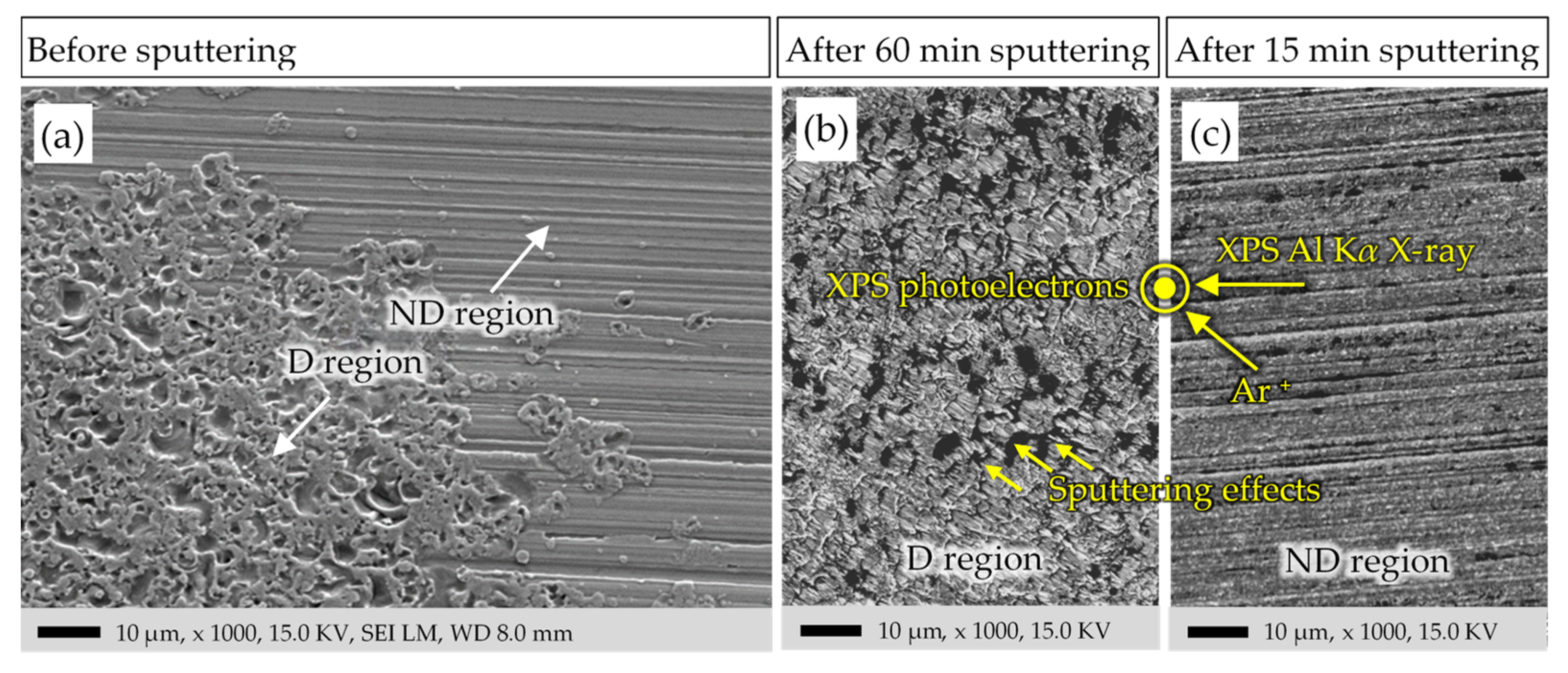
Figure 10a shows the typical topography of the D and ND regions before Ar
+-sputtering. The images of the sputtered areas of the D and ND region are shown in
Figure 10b,c, respectively. Although the sputtering time for the D region is four times longer than for the ND region, the signs of the electrical damage on the surface are still obvious. This agrees with the XPS measurements, which show that after 60 min sputtering in the D region, the content of Fe
3C is still 3.5-times higher than that of the ND region after 15 min.
The angle between the incident Ar
+--beam and X-ray beam and the surface plane is 45° for each pair of them. The XPS analyzer is located at a normal angle to the sample surface (
Figure 10). The effects of material sputtering in
Figure 10b, corresponding to the Ar
+-beam gun direction, is visible. The 60 min Ar
+-sputtering in the D region has drastically changed the morphology of the sample surface. However, 15 min of Ar
+-sputtering in (
Figure 10c) was not enough to eliminate or alter the surface morphology. The parallel lines in the ND region in
Figure 10a are those due to the bearing manufacturing process, with a measured peak-to-valley distance of around several hundred nm.
5. SEM and EDS Results with the FIB Process
In scanning electron microscopy (SEM), a focused beam of electrons with an energy of e.g.,
E0 = 15 keV sweeps the sample surface in a raster grid. The scattered electrons with different energies are counted via an electron detector for each point on the sample to determine the contrast of a corresponding pixel in the output image of the SEM. The incident electron from the electron beam either deflects its path due the elastic scattering via the electric field of the atomic nucleus and returns from the surface as “back-scattered electron BSE”, or finally strikes an electron of an atom as inelastic scattering, releasing it from its atomic orbit as “secondary electron SE”. Leaving the surface, the SE may be detected by the
Everhart–Thornley electron detector (ETD) and contributes to building up the secondary electron image (SEI) [
61]. The SE leaves a vacant position in the orbit of the atom. Other electrons of that atom, in outer orbit positions with higher energies, immediately fill the vacancy, thereby releasing the corresponding energy difference as X-ray photons. The X-ray, measured by an X-ray detector, builds up an X-ray spectrum for each sampling point. Unlike SE and BSE images, the characteristic X-rays give exact information of the composing elements in the energy-dispersive X-ray spectroscopy (EDS).
The information obtained from the sample is not limited to the diameter of the incident beam
[
61]. It is gathered from a volume that is 100 to 1000 times bigger than
. This drop-shaped “interaction” volume differs in size for SEs, BSEs, and X-rays. The SEs have much lower energy levels < 50 eV with a distribution peak at ca. 2–5 eV and are emanated only from a shallow depth of the surface up to ca. 100 nm [
61]. As such, the SEs are more suitable for a topographical contrast image of the surface. The BSEs have much higher energies, from 50 eV to the beam energy
E0, with a distribution peak close to
E0 and a larger penetration depth up to ca. 1 μm. Hence, the BSEs are more for suitable a compositional contrast image. The characteristic X-rays give compositional information of an interaction volume with a depth up to ca. 5 μm [
61]. The more electrons are collected by the detector for a pixel, the brighter that pixel is in the SEM images of the SEs and BSEs. A change of contrast of the pixels in an SEM image usually gives useful information on the investigated specimen. Several factors contribute to a good image contrast. The crystal orientation of the topography to the incident beam direction, the tilting of the sample surface with respect to the incident beam direction and to the detector surface, the atomic number
Z and density of the composing elements, the electrical conductivity of the surface due to charge accumulation, the magnetic field strength, and other factors that affect the amount and direction of the scattered electrons toward the detectors. Among these influencing factors, SE images are very sensitive to the surface topography, while BSE images are very sensitive to the atomic number of the composing elements. The SE images show generally steep surfaces, edges, and borders of protrusions brighter than flat areas. The BSE images show the areas with higher atomic number
Z as brighter than the areas with lower
Z.
We inspected the surface of the fluted raceway via SEM (
Figure 11). The fluted region D in the SE image of
Figure 11a looks brighter due to the higher roughness when compared to the non-damaged region ND. The SE image of
Figure 11b, derived from the EDS software (INCA Energy Software 350, version 4.15), shows the border of the damaged and non-damaged region D and ND, respectively. The high contrast between the edges and the flat area is filtered. However, the holes in the damaged area are much darker compared to the asperities due to the lack of incident electrons reaching the holes. The bearing current, passing through the ball-raceway interface, causes locally strong
Joule heating in the electrically high-resistance
a-spot contacts due to the very high local current densities, leading to melting and even boiling of the surface at the
a-spots, hence damaging the surface (
Figure 11b). The electrical bearing current, by its magnetic self-field, also slightly magnetized the ferromagnetic ring sample structure. Due to this remanent magnetic field, SEM was challenging. A system with a compensation field was used to cancel the effect of the sample magnetic field on the SEM measurements. The track radius of the raceway and the corresponding curvature form of the track surface makes the SEM challenging as well. To optimally focus the electron beam, many trial-and-errors attempts had to be made.
The method of Focused Ion Beam (FIB) excavation was employed (
Figure 11b–f) to mill a trench at the border between the damaged and non-damaged regions D and ND. The sidewall of the trench is examined, using SEM to inspect the composing layers on the surface. The FIB-milling proceeds as follows: First, a band of 1 μm thick platinum (Pt) layer is deposited on the surface as a protective layer against the excavating Ga-ion beam. Then the trench is milled via the focused Ga-ion beam up to the Pt-band (
Figure 11d). At the beginning of the FIB-process, for a coarse-milling the Ga-ion beam is wide and with high energy in order to speed up the milling process, but this results in a vague SEM image of the sidewall. Hence, with a FIB-fine-milling, the cross-section is polished via a narrow Ga-ion beam with lower energies, giving a clear view of the stacked layers (see
Figure 11f). Each FIB process takes about 6 h.
Despite this technique, SEM could not show a distinct oxide layer on the damaged raceway. Between the deposited Pt layers and the bulk steel, only signs of surface damage are visible. Apart from that, the difference between the damaged and non-damaged region is insignificant. A white layer between the Pt layer and bearing surface appeared that could not be explained. Further investigations showed no sign of this layer. The edges in the SE images of
Figure 11d–f appeared brighter, as expected, due to the edge effect. The reason that the upper-right edges of the asperities are brighter than the edges on the other directions is due to the position of the electron detector on the upper-right side of the sample.
The EDS is used to determine the chemical composition of the surface in
Figure 12,
Figure 13,
Figure 14,
Figure 15,
Figure 16 and
Figure 17. The depth of the characteristic X-ray for an element is calculated from [
61]:
where
Rx is characteristic X-ray penetration depth in μm,
ρ is material density in g/cm
3,
E0 is incident electron beam energy, and
Ec is the critical excitation energy, both in keV. The “characteristic” X-ray penetration depths for Fe, O, and C are calculated in
Table 4. The term “characteristic” is skipped in the following.
In
Figure 12a, six points are selected on the sidewall of the trench in
Figure 11e. The visually distinguishable domains are indexed with 1 to 3, from surface-to-bulk, respectively. On the top of layer 1 is the deposited Pt layer, which is beyond the scope of this study. For each visual domain, two points are measured, labeled with a and b, via the EDS. The results are shown in
Figure 12c. Note that Pt and Ga are the contaminations of the FIB process. The trend curves of C, O, and Fe with increasing depth are plotted in
Figure 12d, indicating that the Fe-concentration increases from-surface-to-bulk, whereas the C-concentration decreases. The changing trend of the concentrations are in good agreement with our XPS measurements.
The EDS elemental mapping of O and Fe in
Figure 12b reveals that the O-concentration decreases from-surface-to-bulk. Each EDS data point represents a drop-shaped interaction volume with a depth of ca. 0.7 μm (see
Table 4), so the EDS results do not necessarily represent the features on the SE image, but also beneath of it. The SEs have an “escape depth” up to 5λ
e ≈ 2.5 nm [
61,
62], where λ
e is the mean free path of the SEs in Fe.
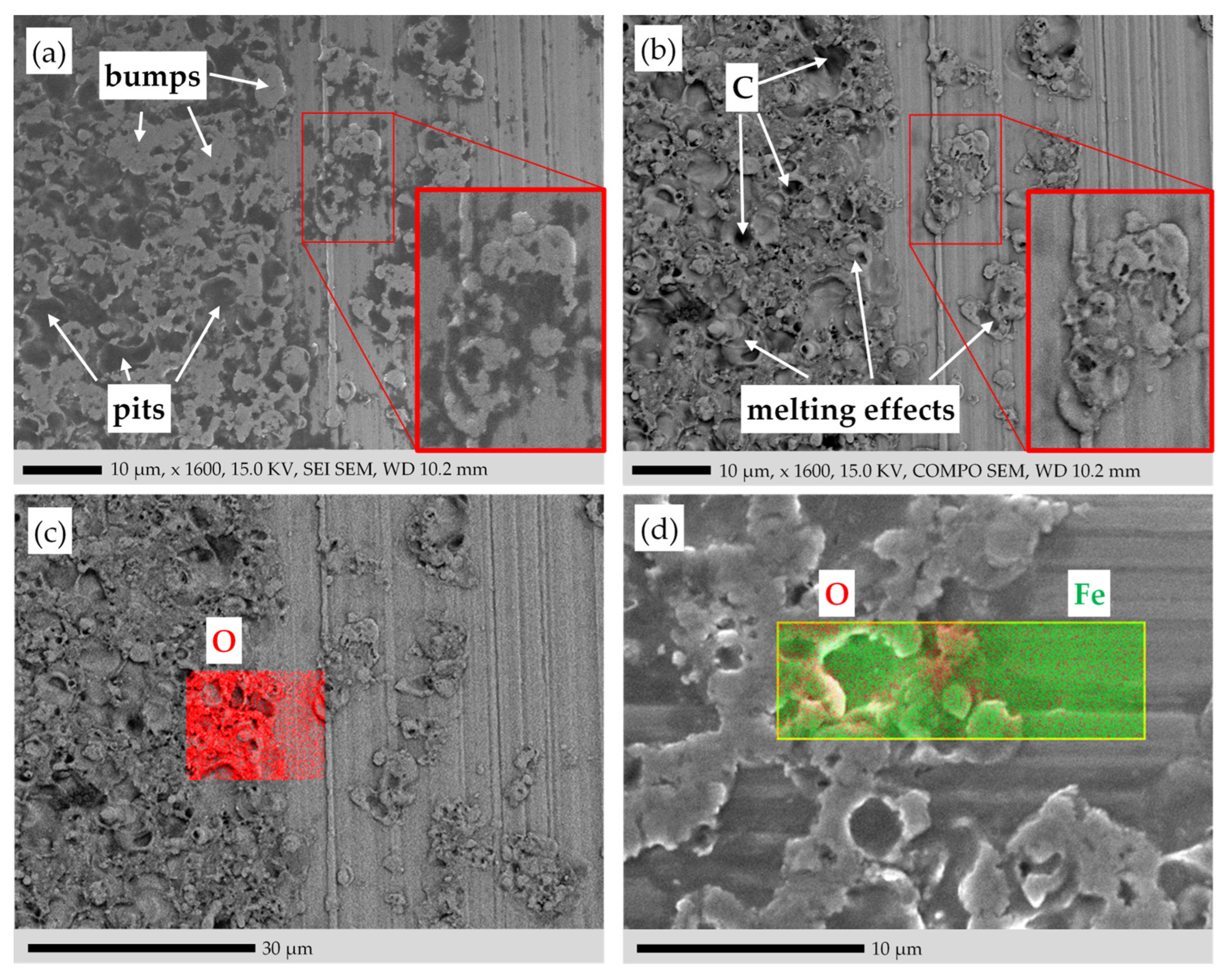
The topology of the surface was further investigated with the SEM analysis via SEs and BSEs in
Figure 13a,b, respectively. Two electron detectors for BSEs were mounted over the sample close to the incident electron beam (
Figure 14), each detecting the BSEs of one side of the beam better than the other side [
61]. The BSE image has two modes of operation: the Topographical Mode (TOPO) and the Compositional Mode (COMPO). The COMPO mode gives a better atomic number contrast for composition, since the intensities of the BSE detectors are added to intensify the atomic number contrast. The TOPO mode gives a better topographical contrast, since the intensities of the BSE detectors are subtracted from each other to intensify the variation of the atomic number with the moving electron beam. Here only the COMPO mode is used. The pits caused by the electric current in the SE image of
Figure 13a are darker than in the BSE image of
Figure 13b. As shown in
Figure 14, unlike the BSE detector, the SE detector is placed at an angle of ca. 30° with the sample plane [
61]. Hence, the SEs, emitted from the pits, may be disturbed by the crater rims of the pits, and do not reach the detector. Due to this “shadow effect”, the pits look darker in the SE image. In the BSE image, for the very deep pits the number of emanated BSEs is reduced, contributing to their darkness. Moreover, the disintegrated burnt lubricant yields carbon (
Zc = 6), entrapped in the pits, and appears darker when compared to the metallic iron atoms Fe (
ZFe = 26).
The EDS elemental mapping is employed in
Figure 13c,d to detect the surface oxide. It is expected that the oxide covers the whole surface, especially at the damaged areas, where the high temperatures due to the electric current flow occurred. The penetration depth of the EDS technique for O is ca. 0.77 μm (
Table 4). The oxide layer exists on the surface in a much thinner depth than 0.77 μm. Hence, the EDS technique cannot inspect the intended oxidized surface exclusively. The EDS results contain information from the deeper regions as well. The O in the elemental mapping is not distributed evenly over the damaged region D. The areas with the higher bumps due to surface damage have a thicker metal layer of previously molten material, resulting in a higher O concentration. In any case, a higher O concentration in the damaged area D is obvious in
Figure 13c,d when compared to the non-damaged area ND.
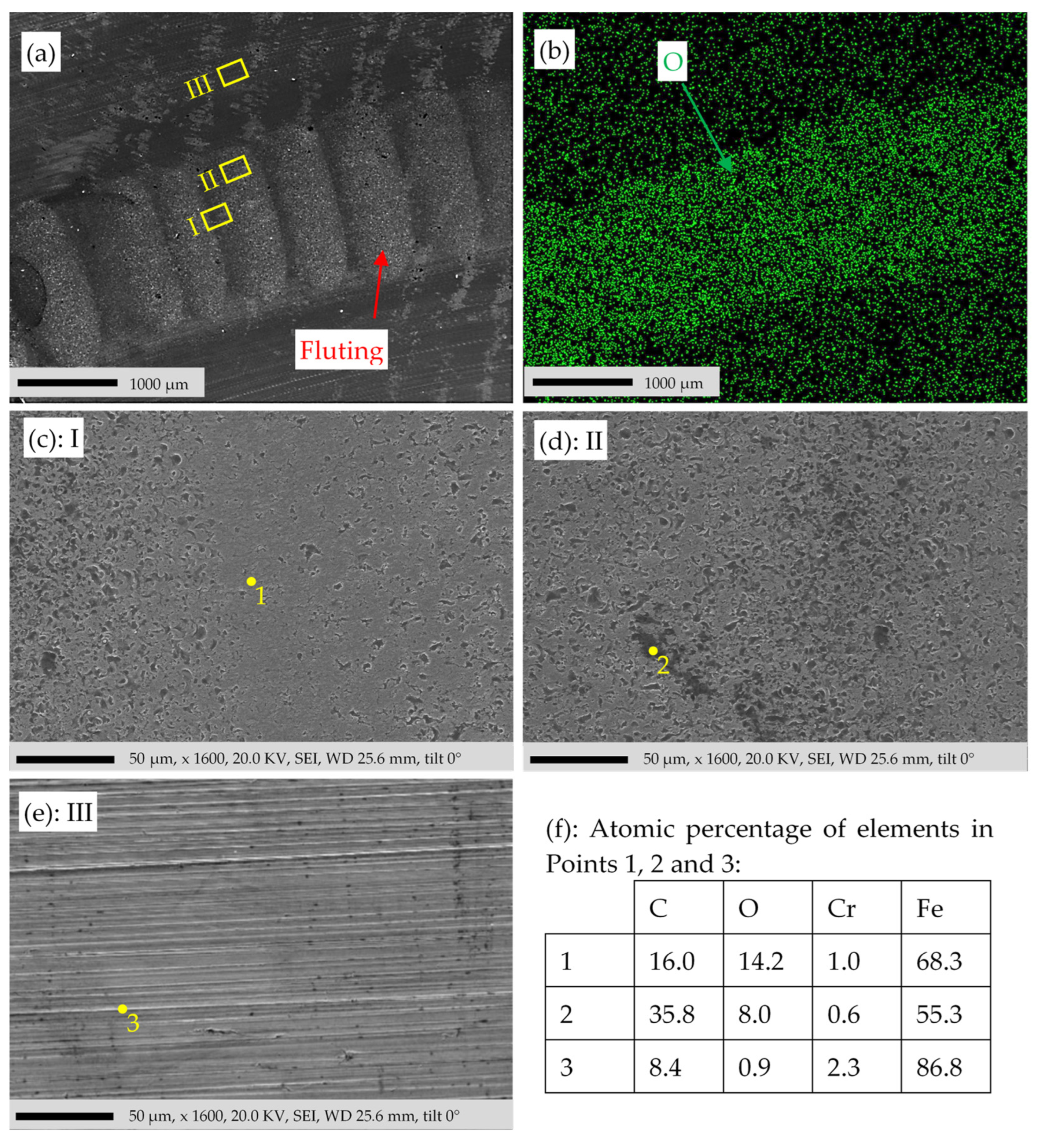
EDS elemental mapping is used for larger areas in
Figure 15 to verify the findings of
Figure 13c,d. Three areas, one on the fluting valley in D, one on the fluting peak in D, and one outside the raceway in the non-damaged region ND, are selected, as shown in
Figure 15a,b. The EDS elemental mappings in
Figure 15c–f show that the averaged atomic percentage of O in area I and II is almost equal at around 21%, which is much bigger than that of area III with only 2.8% outside the flutings in the non-damaged region.
To verify the findings of
Figure 15, another SEM/EDS investigation was performed in
Figure 16.
Figure 16b shows a higher concentration of O in the damaged region D. Unlike
Figure 15, in
Figure 16c–e, EDS spectra are measured at three points (1, 2, and 3) in the regions I, II, and III, respectively. The concentration of C in Point 1 is higher than in Point 2, suggesting that Point 2 is in a deep pit located on the damaged surface D, where a significant amount of C is trapped as a result of the burnt lubricant. A higher O concentration in Point 1 compared to Point 2 is due to the difference in the C concentration and due to the height difference. The bigger heights of the bumps compared to the pits result in their longer exposure time to the high temperatures during the bearing current flow, leading to more oxidation. Point 3 outside the damaged region has a much lower O concentration, a much higher Fe concentration, and a relatively lower C concentration, as listed in
Figure 16f.
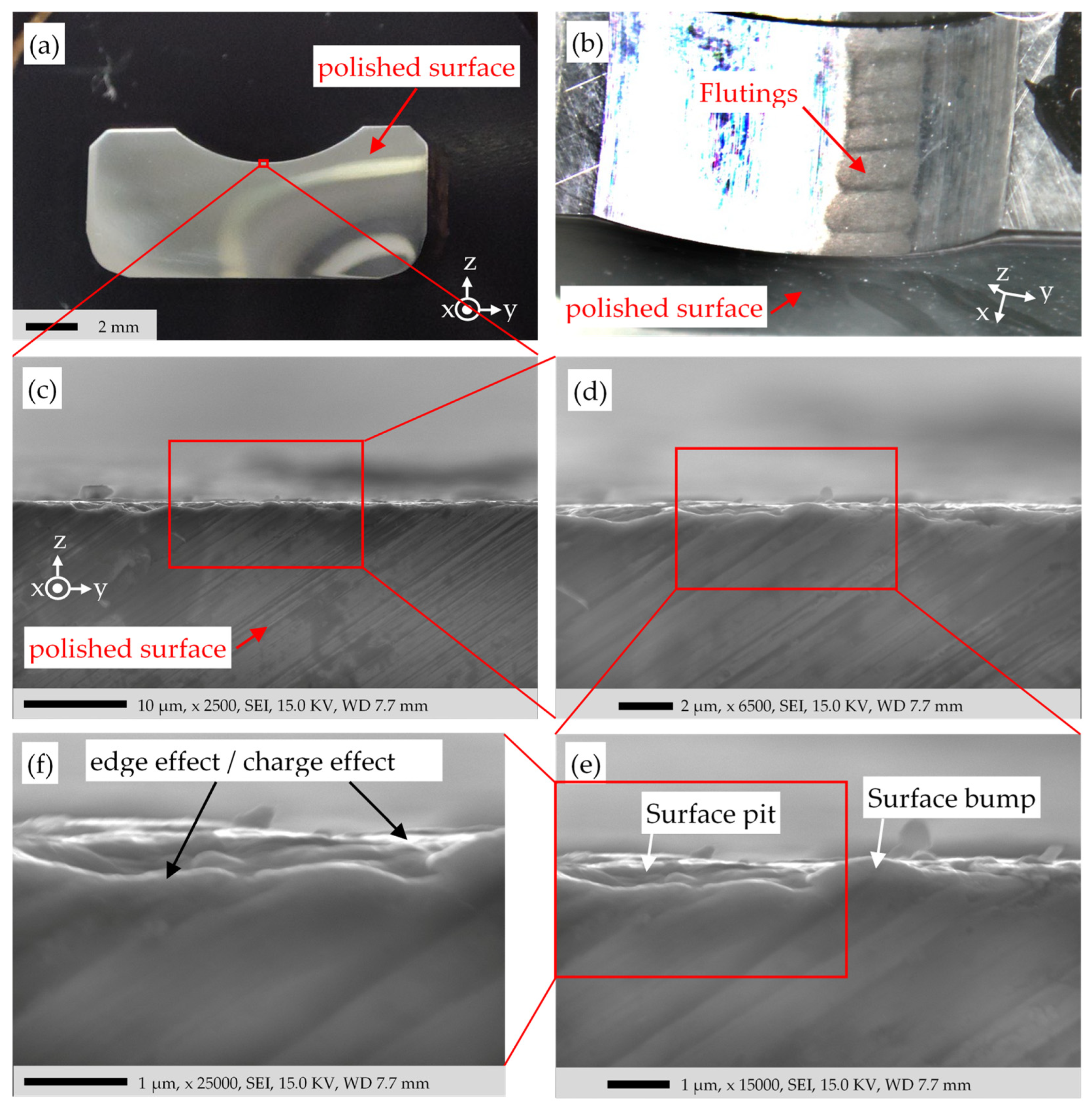
To investigate the surface characteristics, like in
Figure 11 and
Figure 12 but without deposited Pt, the whole cross-section of the bearing ring is cut via an EDM wire cut. Thus, the bearing ring is divided into four parts. For one part, the cut surface (
Figure 17) is polished with sandpaper (
Table 1) to clean the surface of cutting-caused contaminants. To protect the edge of the damaged surface and to get a finer flattening of the cross-section surface, another part of the cut surface (
Figure 18) was finely polished with the polishing machine in
Table 1 with SiC paper with the following grit numbers: P120, P220, P320, P500, P1200, P500, P4000; each for approx. 2 min.
The SEM image of
Figure 17a does not show any distinct layer on the surface related to the oxide. The bright color shining on the edge may be due to the “edge effect” of the emitted SEs in SEM technique [
61]. The SEs are emitted much more from the edges of a protrusion than from a flat region. This effect arises because the SEs have shorter “escape paths” from the SE interaction volume to the surface. The sample is metallic (conductive), and the sample holder is electrically grounded, so the electrons cannot accumulate in any part, connected electrically to the bulk. Any electrically insulated particle on the surface appears shiny due to the “charging effect” [
61]. The insulating oxide may result in a charging effect on the surface, causing the shiny color. Two points are selected for EDS analysis: Point 1 on the edge of the sample targeting the damaged surface and point 2 on the bulk steel.
Figure 17b shows, by 5.4 times and 2 times, respectively, higher O and C concentration on the damaged surface (point 1), compared to the bulk steel (point 2).
The SEM image in
Figure 18e shows the typical bumps and pits due to the electrical damage.
Figure 18f shows no clear margin between the surface layers and the bulk steel. The XPS results in
Figure 9 have shown the composing layers on the surface. The iron oxide concentration decreases exponentially, moving inward from surface-to-bulk. A pronounced change and a visible border line between the oxide and bulk steel is therefore not expected in
Figure 18f. The edge effect may cause the shiny regions in
Figure 18f, and/or the insulating oxide on the surface may accumulate the electrons from the incident beam, resulting in an increased SE emission and the shining color. This charge effect is more probable visible in
Figure 19.
Figure 19 is the same sample as in
Figure 18 but rotated to take images from the damaged surface and via BSEs. The typical surface damages are seen in
Figure 19, similar to those in
Figure 11b and
Figure 13d. The dark spots on the surface are attributed to the deep holes or the accumulation of C. The generally brighter color of the surface compared to the bulk may be due to the insulating oxide layer (charge effect) and/or due to a reduced amount of incident electrons reaching the bulk steel.
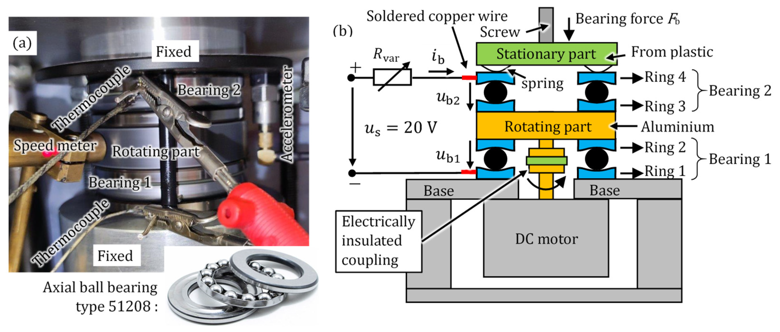
6. Summary
The electrically damaged surface of a fluted raceway of an axial ball bearing type 51208 was studied. An DC apparent bearing current density of 3.85 A/mm2, which is ten times bigger than the safe limit value 0.3 A/mm2, at 400 N axial bearing force and a grease lubrication with Arcanol MULTI3, had generated severe fluting after 24 h operation at 1500 rpm. The properties of the electrically damaged area of the raceway within the fluting pattern, influenced by the degraded lubricant, in comparison with the non-damaged area was closely investigated by light microscope, WLI, SEM, XPS, and EDS.
WLI showed high roughness peaks on the surface. The motif analysis showed that the surface roughness was irregular and stochastic. These findings support our hypothesis that the very high bearing currents lead to a roughened surface, causing mechanical contact points between the raceway and the ball, even at an elevated speed of e.g., 1500 rpm, where typically full lubrication was expected.
SEM showed the signs of locally molten electrical contact points (a-spots). The residual carbons from the degraded lubricant are trapped in the surface pits and can be seen in dark contrasts in the BSE images. These findings support our hypothesis that the locally high current density results in excessive Joule heating, which leads to local melting of the steel. This heat obviously burns lubricant molecules, explaining the carbon deposits and the blackening of the lubricant. A distinguishable border between the oxide phases and the bulk of bearing was not seen in the SEM images after the FIB or the cut-and-polish procedures.
The XPS and EDS results proved the existence of surface oxide phases. The XPS also showed the high share of iron carbide on the surface in the damaged area. Skipping the surface contaminations and moving from-surface-to-bulk, the atomic concentration of iron oxide phases decreases, the carbide increases first and then slightly decreases, and the metallic iron increases. This supports our hypothesis that the electrical current flow must punch the insulating oxide layers at distinct changing contact points. The electrical current flow chemically changed both the lubricant and the raceway surface.
Figure 20a gives a schematic view of the intact bearing surface without current flow, hence the non-damaged region ND, where the “native oxide” due to exposure to air results in a thin oxide layer. On the contrary,
Figure 20b illustrates the compositional surface changes schematically due to current flow in the damaged region D, along with the surface topographies, where the asperity peaks make the mechanical contacts, and the carbon residues are trapped in the surface pits. Not all the mechanical contacts cause electric contacts (
a-spots) due to the insulating oxide layer, which mostly covers the ball-raceway interfaces. Hence the fluting pattern generation may be influenced by the local abrasion of the oxide layer. Its periodic pattern is so far explained by micro-vibrations of the contact partners with peak-to-valley depths of up to 3 μm in our case.

 ,
, 


