

Combined Observer-Based State Feedback and Optimized P/PI Control for a Robust Operation of Quadrotors

Group: Distributed Control in Interconnected Systems, School II—Department of Computing Science, Carl von Ossietzky Universität Oldenburg, D-26111 Oldenburg, Germany
*
Authors to whom correspondence should be addressed.
Axioms 2024, 13(5), 285; https://0-doi-org.brum.beds.ac.uk/10.3390/axioms13050285
Submission received: 27 February 2024
/
Revised: 9 April 2024
/
Accepted: 18 April 2024
/
Published: 23 April 2024
(This article belongs to the Special Issue Advances in Mathematical Methods in Optimal Control and Applications)
Abstract
:This paper deals with a discrete-time observer-based state feedback control design by taking into consideration bounded parameter uncertainty, actuator faults, and stochastic noise in an inner control loop which is extended in a cascaded manner by outer PI- and P-control loops for velocity and position regulation. The aim of the corresponding subdivision of the quadrotor model is the treatment of the control design in a systematic manner. In the inner loop, linear matrix inequality techniques are employed for the placement of poles into a desired area within the complex z-plane. A robustification of the design towards noise is achieved by optimizing both control and observer gains simultaneously guaranteeing stability in a predefined bounded state domain. This procedure helps to reduce the sensitivity of the inner control loop towards changes induced by the outer one. Finally, a model-based optimization process is employed to tune the parameters of the outer P/PI controllers. To allow for the validation of accurate trajectory tracking, a comparison of the novel approach with the use of a standard extended Kalman filter-based linear-quadratic regulator synthesis is presented to demonstrate the superiority of the new design.
Keywords:
robust control; linear matrix inequalities; interval methods; extended Kalman filter; linear-quadratic regulator design; proportional–integral controllerMSC:
93B52; 93C73; 93D09; 93B351. Introduction
The use of quadrotors has become remarkable nowadays [1,2,3], because of their capability to fly in both small indoor areas and rough outdoor environments which, for example, helps to perform rescue missions in case of disasters or for agricultural monitoring.
Since quadrotors are characterized by under-actuated dynamics [4] and their models show nonlinear coupling between the different degrees of freedom, the literature presents nonlinear control approaches that deal with such models with parameter uncertainties as in [5,6,7], where in the latest, the authors have used an adaptive barrier function to ensure fast convergence in the presence of uncertainties in the model. From the nonlinear control theory, the authors in [8] have considered an attitude representation given by Modified Rodrigues Parameters (MRPs) exploited by a passivity-based scheme to stabilize the attitude dynamics that is combined with a differential flatness-based approach for the position dynamics to linearize the system via feedforward control.
The robustification against disturbances has also been studied in the literature [9]. In addition, the authors of [10] have proposed a backstepping method interfaced with sliding mode control for position and attitude control in the presence of external disturbances, while the estimation of controller parameters was assured by using adaptive laws. In addition, the upper limits of the attitude perturbations were estimated with the same approach. For the same purpose, the authors in [11] have considered a nonlinear Proportional Integral Derivative (PID) controller where its parameters have been tuned using a Genetic Algorithm to minimize a multi-objective output performance index. Compared to the Linear PID, the attitude loop has shown better robustness against measurement noise and disturbance in contrast to the position loop.
Another challenge that has been tackled in the literature is dealing with actuator faults, as in [12], where the authors have combined model predictive control and reinforcement learning to detect and compensate faults of a quadrotor during trajectory tracking. The same objective has been treated with the help of linear control theory in [13,14,15], where the authors exploited the linear matrix inequalities (LMIs) tool to solve problems for different purposes such as fault diagnosis or state estimation, while the authors in [16] have exploited a Kalman filter to propose a fault detection and diagnosis scheme to detect and isolate actuator faults in presence of external disturbances. In contrast to this, the authors of the reference [17] have exploited an extended Kalman filter. In [18,19], the authors have exploited a zonotopic unknown input observer and the zonotopic extended Kalman filter for state estimation, respectively.
The state estimation is required if there is no possibility to measure a physical quantity. The estimate then serves as a substitute for non-measured signals, and it is then used by the control law as in [20] where the authors have addressed the trajectory tracking problem using saturated proportional–derivative (PD) control laws and disturbance compensation, in addition to an observer-based attitude tracking control that has been established in a separate design phase. The same procedure has been exploited in [21], where the authors have used the solution of a type of generalized Sylvester equation to parameterize a full-order observer-based controller for a quasi-linear system. Moreover, the authors have demonstrated the validity of the separation theorem since they have considered perfectly known time-varying parameters and state values.
Although several papers have been published that tackle the design of controllers and observers separately, little attention has been paid to a joint design if the modeled systems are nonlinear or depend on uncertain parameters. To the best of the authors’ knowledge, an example of such kind of research can be found in [22] where the authors have considered time delays and input disturbances in their design phase. In [23,24], the authors have exploited the LMI framework in order to simultaneously design a controller and observer that guarantee stability and robust performance despite the occurrence of actuator faults, model uncertainty, nonlinearities, and measurement noise and that only require the tuning of two parameters. This joint design of control and observer gains is justified by the illustrating example given in the 2nd section in [24]. It illustrates the fact that the separation principle of control and observer design no longer holds for linear systems with bounded parameter uncertainty. This is equally true for the case of nonlinear systems. To keep the control design as simple as possible, we investigate the following design procedure in the current article: The control architecture is divided into two parts so that a robust LMI-based approach is employed for the inner loop, whilst optimized proportional and proportional–integral controllers are used for the cascaded outer loops. Hence, the purpose is to evaluate the time-domain performance of the mutual impact between the cascaded control loops while enhancing flight accuracy despite measurement noise and external disturbances such as wind or component wear. Moreover, it is shown that the proposed design procedure clearly outperforms the control accuracy achievable by a standard tuning approach for this type of control structure, both in the unperturbed case and in a setting in which large actuator disturbances act on the closed-loop system dynamics.
This paper is organized as follows. In Section 2, the quadrotor model is introduced. In Section 3, the control methods and the parametrization of the state trajectories are described. In Section 4, simulation results are presented. Finally, the paper is concluded in Section 5 with a discussion of the obtained results and an outlook on future work.
2. Quadrotor Modeling
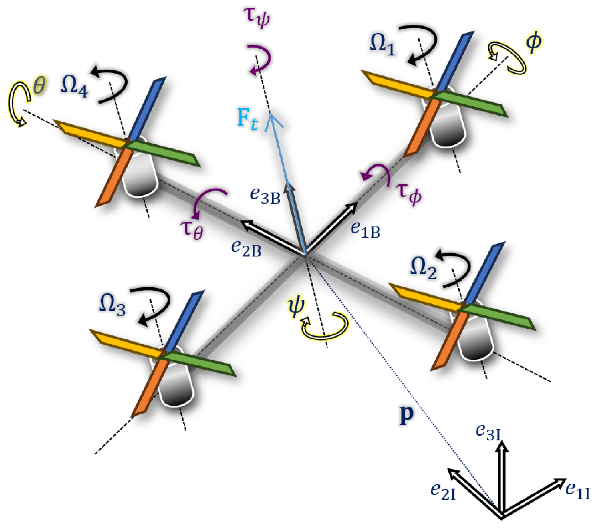
To be able to derive the nonlinear dynamic equations of the quadrotor, the rotation from earth’s inertial frame () to the body fixed-frame () is considered as described in Figure 1 with the use of the ZYX convention [25].
According to [26], the Newton–Euler formalism is employed which is less complex and less difficult to compute compared to the Euler–Lagrangian approach [27]. For modeling and control purposes, the general dynamic model of a quadrotor is subdivided into two parts. The first one is the attitude sub-model represented by
and the second is the velocity sub-model represented by
with denoting, respectively, the roll, pitch, and yaw angles. The position of the quadrotor in the earth-fixed coordinate frame is described by the vector denoting, respectively, the longitudinal, lateral, and vertical axes. The parameter is the rotor inertia, while , , and are the diagonal entries of the quadrotor’s inertia matrix. The parameter l is the length of the lever, while m and g are, respectively, the mass and the Earth’s gravity.
The total thrust is the sum of the thrusts of each of the rotors, where represent, respectively, the roll, pitch, and yaw torques, all depending on the rotor speeds , according to
Additionally, the variable is considered during the parametrization of the inner loop as a fictitious stochastic disturbance. However, when optimizing the outer control loops, and when performing the system simulation, the dependence of on the speeds of the four rotors is accounted for by the relation
with the constants b and d being, respectively, the thrust factor and the drag factor.
3. Quadrotor Control System
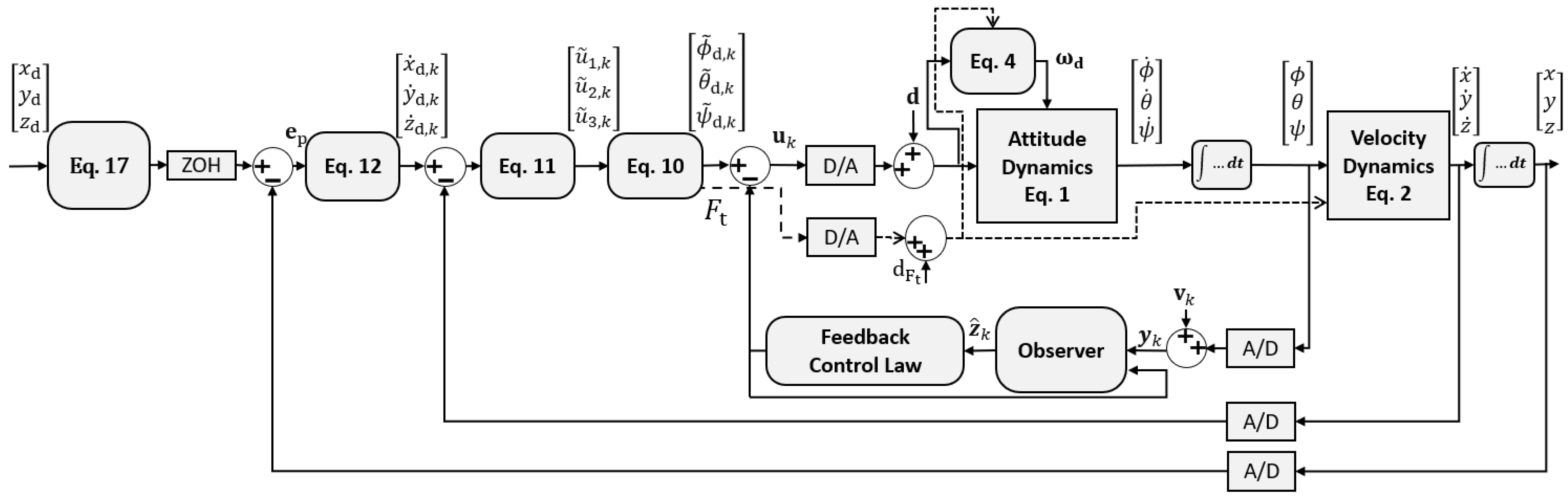
To design the control system for the quadrotor, two main control loops have been constructed as cascaded outer and inner loops, as shown in Figure 2. The two outer ones encompass the position and velocity control loops that ensure the fulfillment of the position tracking mission, whilst the inner-most is responsible for attitude tracking.
Remark 1.
This structure ensures that the outer position and velocity control loops do not negatively impact the overall system stability as long as the quadrotor is operated with reference trajectories that lead to system states that are compatible with the state constraints resulting from the polytopic uncertainty model derived in Section 3.1. If this property is satisfied, the combination of the underlying LMI-based state feedback in the inner loop with the P/PI outer feedback loops ensures asymptotic stability of the overall control system. This statement is equally true for a nominal system behavior without actuator faults and for scenarios in which actuator faults are present as long as the latter do not lead to a loss of controllability.
3.1. Parametrization of the Attitude Control Loop Using an LMI-Based Method
To guarantee robust performance despite actuator faults, model uncertainty, nonlinearities, and measurement noise, the authors of [23] have employed a novel iterative LMI approach to design a discrete-time observer-based state-feedback controller in the presence of both bounded parameter uncertainty and stochastic noise.
Reformulating (1) as a discrete-time quasi-linear state-space representation yields
where the explicit Euler method with a sampling time ms is used in this paper. Moreover, the state vector is which is assumed to be bounded by a priori known intervals, which are compatible with the reference trajectory to be tracked. The input vector of the inner loop is denoted by . Additionally, and are, respectively, the output vector and actuator fault vector acting additively on . Finally, is the state-dependent system matrix, is the input matrix, is the disturbance input matrix, coupling the process noise with the system dynamics, and is the output matrix. A standard normally distributed random output noise is taken into consideration with its standard deviation specified by the matrix .
In a practical application, the actuator faults could manifest themselves in different manners like a blocking, saturation, or efficiency loss of the physical actuators. Hence, a discrete-time integrator actuator fault model is taken into account to be able to estimate such faults , while these estimates are used for the compensation.
The occurrence of actuator faults influences the total thrust and the deviation is represented with . This deviation is transmitted to the attitude dynamics through . This deviation is neither estimated nor compensated in the closed inner loop. However, the influence of such faults is assumed to be sufficiently small due to its multiplication with the small drag factor.
Compared to what has been addressed in [28,29], the variable is taken into consideration in the algorithm of the proposed iterative LMI-based controller design as a fictitious (random) disturbance instead of an alternative compensation of its influence in the control law formula that would be possible in a least-squares sense.
For the sake of state and disturbance estimation, consider a linear time-invariant full-state observer that is designed on the basis of the discrete-time state-space representation
where and are the nominal system matrices evaluated in the hovering state.
This observer provides the required information to realize the inner control loop with the estimated vector in the form
where the matrix replaces a pre-filter which could be used as an alternative to the following outer loop optimization to reduce tracking errors during transient phases. The vector is determined in Section 3.4 by an approximation around the hovering state (assuming sufficiently small angles in roll, pitch, and yaw).
Considering the estimation error model and combining it with the discrete-time model of the observer-based inner control loop leads to the augmented state- space representation
with , . This augmented system model takes into consideration both process and output noise, where the latter was not explicitly considered in the previous work [23].
Thereafter, a selection of interval bounds for the states included in and forms the basis for building a polytopic domain with extremal vertices that are involved in an optimization task that exploits the Lyapunov stability method as described in [23], generalized by both a placement of poles into the desired regions and a robustification against noise. Therefore, the design algorithm starts by choosing a radius r and a center of a circle in the z-plane corresponding to the desired closed-loop eigenvalue domain. The design provides the controller gain and the observer gain that are optimized jointly. Thus, the stabilization of the nonlinear system in a predefined operating range is ensured. The computation effort of this algorithm is not critical from a real-time perspective since it is executed offline.
3.2. Extended Kalman Filter-Based Linear Quadratic Regulator Design
An alternative control method to parametrize the inner loop is to employ an extended Kalman filter (EKF) to estimate the states and actuator faults, so that this information can be used by the linear quadratic regulator (LQR).
As shown in the paper [23], additive Gaussian process noise is considered in Equation (5) as well as in the integrator disturbance model employed for actuator fault detection characterized by their corresponding mean values (being zero) and their covariance matrices.
The EKF approach consists of two parts, where all computations are performed online. In the prediction step, the expected value and the covariance of the states and actuator faults are propagated up to the point in time where the next measurement data become available. Then, the innovation step is employed to update the expected value and covariance.
The mean values and covariance matrices are estimated recursively by an alternating sequence of prediction and innovation steps. These estimates are fed back using the same structure of the control law as shown in Equation (7). Note that the controller gain is computed by a minimization of an integral quadratic cost function for which the weighting matrices are the available tuning factors.
This method does not provide a guaranteed proof of stability for nonlinear systems since the computation of the controller and observer gains are made separately, and the separation principle of control and observer design is no longer valid in this case.
Note that the use of an online gain scheduling [30] or solutions on the basis of state-dependent Riccati equations could be used to enhance the reliability of this approach [31]; however, it comes with the price of a significantly higher implementation and computational effort than the proposed methodology presented in the previous section.
3.3. Velocity and Position Control Systems
The velocity control loop provides set-point information for the output (i.e., the angles) of the inner-most sub-model which themselves are the inputs of the velocity sub-model according to Equation (2). For the implementation of the velocity controller, the expressions (2) are approximated around the operating point (hovering state) by using small angle approximations of the trigonometric functions, i.e., , , where denotes either the roll, pitch, or yaw angles. In addition, the yaw angle is set to zero since it is not necessary to achieve the desired velocity profile. Finally, this leads to the virtual controls
which can then be used to determine the set-points
as described in [26].
In the equations above, the virtual controls ,, and are calculated by using the proportional control laws
where the subscript “” refers to the corresponding desired signals.
The outer-most position control loop makes use of the discrete-time PI controllers
which are implemented with the help of a forward Euler discretization with as the sampling time.
Since the quadrotor is considered to be symmetric, the desired dynamics for each Cartesian position coordinate are assumed to be the same. This justifies the use of identical control parameters for each of the coordinates in (11) and (12), where the actual values are obtained numerically by minimizing the square cost function
Here, the constant is the index of the final simulation time. The variable is the number of all components of the vectors. The total input is . The variables and are strictly positive weighting coefficients chosen equal to one in this study; is the position error and is the attitude error.
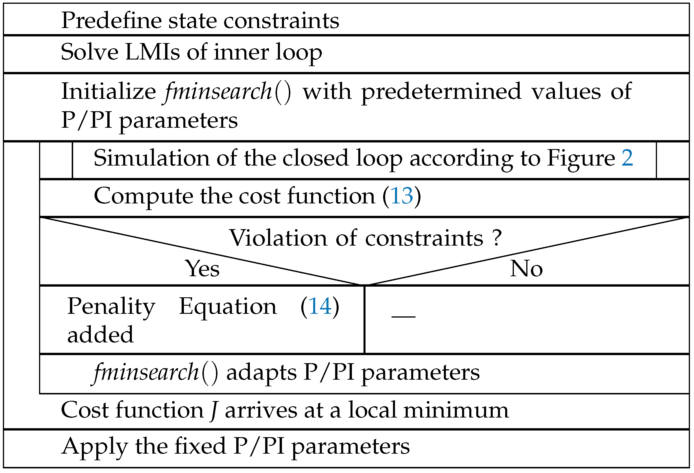
The function in Matlab [32] is used in this article to obtain suitable P/PI parameters by an iterative simulation in Simulink. Using the Nelder–Mead simplex algorithm, it returns a local minimizer of the cost function J near the initial values of ,, and which are typically predetermined by a few iterations in an trial-and-error approach. Note that this optimization is firstly used for a fault-free system model. In such cases, the minimization reduces the deviation between the actual system behavior and the desired reference trajectories. In addition, it is possible to include certain fault scenarios in the simulation model used for this model-based optimization. Then, the outcome is a selection of the P/PI gains that does not only enhance the nominal system behavior but equally reduces the sensitivity of the closed-loop dynamics against actuator faults.
Note that a further penalty could be added within the summation of the cost function (13) in cases in which the state bounds included in (8) are violated due to inappropriate P/PI parameters. For instance, the angular velocities
could be penalized by choosing a higher value of the corresponding weighting coefficient at all times outside the bounds from which the polytopic model of the LMI-based synthesis was derived. The index l means the components of the angular velocities vector. The algorithm in Figure 3 shows the procedure, and it is described using Nassi–Shneiderman diagram.
3.4. Trajectory Planning
In order to specify smooth position responses, and to avoid a specification of unrealistic steps as the desired output signals, a trajectory planning procedure is used. It is based on a product of time-dependent Bernstein polynomials of degree
defined on each time interval , with
and a vector of constant coefficients
According to [33], the coefficients (17) are chosen so that the time derivatives of the desired state trajectories
are at least three times continuously differentiable at the points . In this way, smooth point-to-point trajectories can be specified, while the choice of allows for a limitation of the desired velocities and accelerations.
As a second type of desired trajectory used in the following section, ∞-shaped curves are employed. They are represented in the form of the lemniscate of Bernoulli, where the parametric equation is given by
with as the half-width of the lemniscate.
3.5. Structural Comparison of the Performance with Nonlinear Methods from the Literature
To evaluate the fundamental properties of the developed approach, it is compared to other nonlinear methods from the literature as collected in Table 1. As a general nonlinear alternative, an observer-based adaptive sliding mode control approach has been selected. The advantage of the proposed methodology can be found in the simplicity of its implementation on the target system (i.e., it keeps a standard linear state feedback in the underlying control loop with an optimally tuned P/PI feedback in the external loops). It should be pointed out that we do not claim at this point to outperform arbitrary nonlinear control procedures in the tracking capability with this linear feedback strategy. In contrast, we would like to emphasize that the robustified design of a linear control approach is significantly more efficient than applying state-of-the-art design principles such as a linear quadratic regulator design in combination with extended Kalman filters. It has to be noted further that our implementation is even less demanding from an online computational point of view than the aforementioned alternative due to the fact that both control and observer gains can be kept constant for the entire trajectory.
4. Simulation Results
In this section, numerical simulation results using Matlab/Simulink, with ODE1 as the solver and a step size of 1 ms which is set for also, are presented. The inner loop is running at 1 khz, and the outer loops are running at s. The parameter values used for the model are shown in Table 2.
Consider firstly a surveillance mission, where the scenario is to take off vertically, go slowly horizontally, and then vertically land. After 22 s, an actuator fault occurs, which leads at the same time to deviations in the yaw torque of Nm, Nm in the roll torque , and N in the total thrust . Those values were chosen to reflect severe faults in this simulation analysis to validate the control procedure for worst-case operating conditions.
To configure the trajectory planning, the degree parameter in Equation (15) is chosen as . So, in the time intervals s, s, and s, the first five vector entries in Equation (17) are chosen equal to the desired initial Cartesian coordinates, and the last five entries are set to the desired final Cartesian coordinates.
Different optimizations of the outer-loop controller parameters are carried out with respect to the control method used in the inner loop. The weighting parameter in the first simulation is . For the LMI-based simulation, the parameters of the PI position controller are obtained as for the proportional gain, and for the integral gain while the value of the P velocity controller is obtained as . For the EKF-based LQR simulation, the values of the PI position controller are obtained with for the proportional gain and for the integral gain, while the value of the P velocity controller is obtained as . The values of the P/PI for the LMI-based method were obtained while testing large initial values for compared to those obtained for the EKF-LQR method, where if far from the initial values, the responses diverge.
The inner-most state feedback is parametrized by using the same values as used in [23], except for the bounds of the angular velocities, specified in rad/s, , , . For the variance of the Gaussian output noise , the value was chosen for all three components, with the matrix in the synthesis phase.
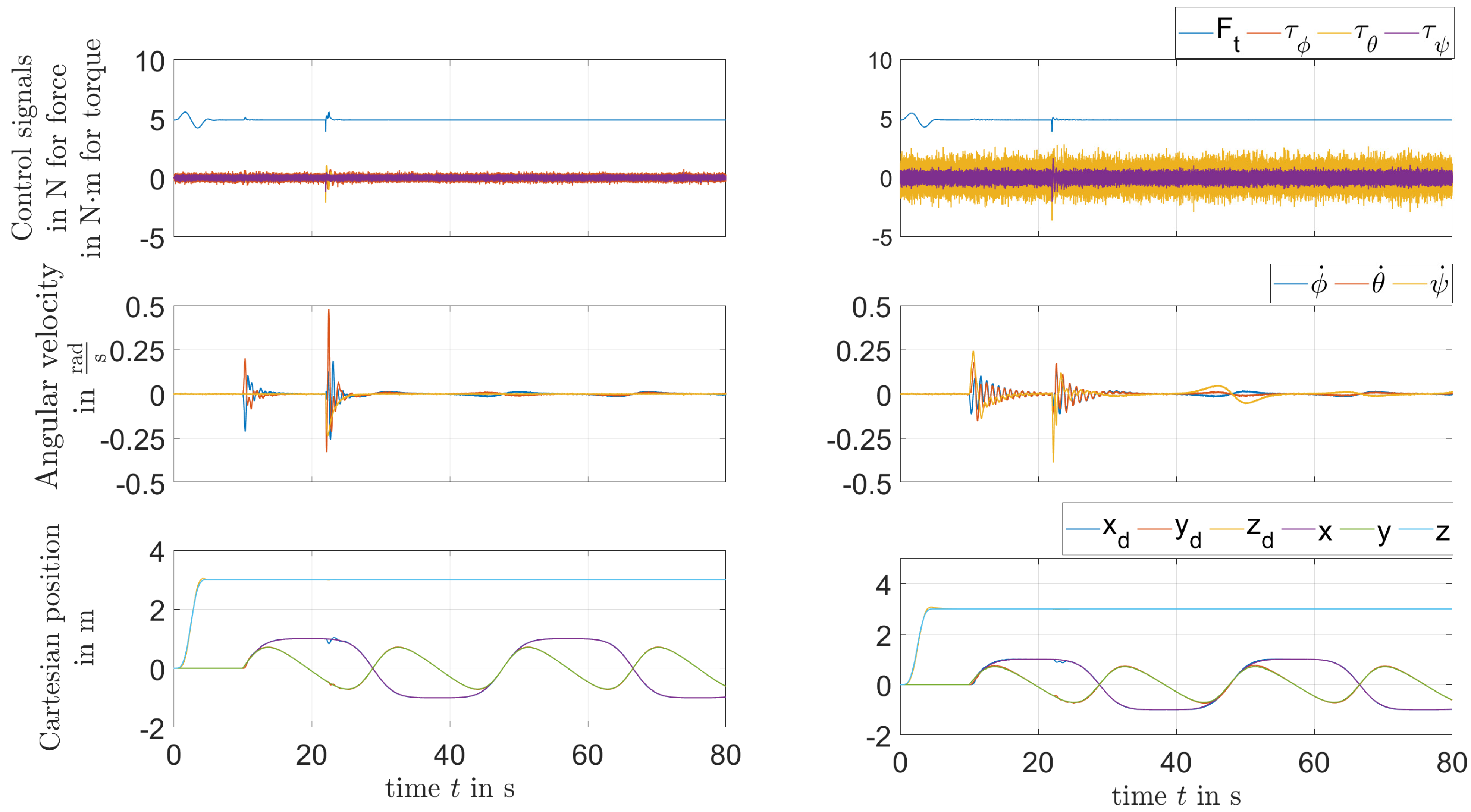
Figure 4 shows the attitude responses. It can be seen that the curves return to a steady state quickly with both methods. In the LMI-based response, throughout s, the yaw angular velocity violates the polytopic model bounds used to represent the state dependencies in Equation (5). The inputs applied to the quadrotor model are shown in Figure 5.
Since the stability condition established in the LMI framework may be conservative, the eigenvalues of the matrix at the times s are checked to be inside the unit circle. By taking the input of the inner-loop, which corresponds the output of the prefilter and the output of the attitude model which are the angles in Figure 2, a linearized model of the inner observer-based control loop is obtained with the help of Matlab’s function. The resulting eigenvalues of the discretized inner control loop are shown in Figure 6, where all eigenvalues are inside the unit circle of the complex z-plane
Although this analysis is still not a strict stability proof due to the time variance of the linearized model, it serves as an indicator for the reliability of the obtained result even in the worst case.
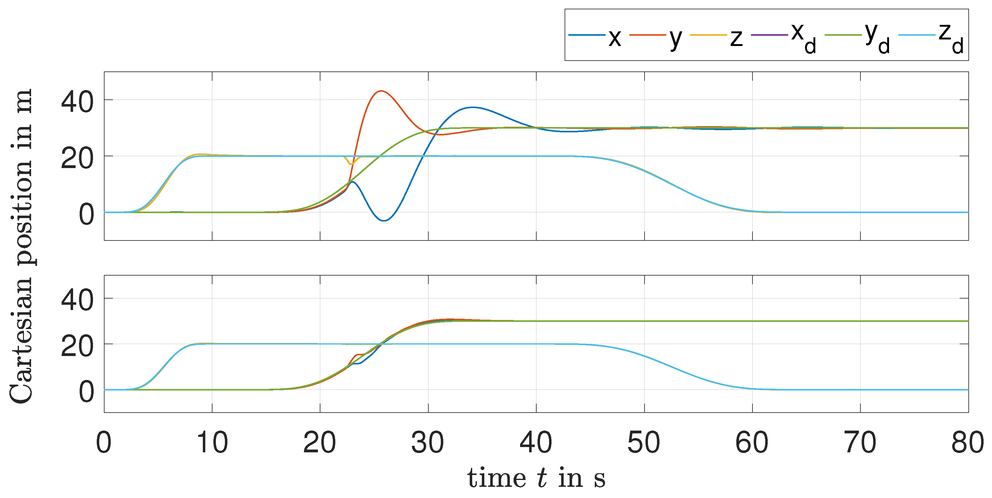
Figure 7 shows the curves of the Cartesian position, where the influence of the actuator faults significantly appears when using the EKF-based method in the inner loop, which leads to huge deviations for the longitudinal and lateral coordinates from the desired trajectories. This behavior is removed in the case of the LMI-based method. The behavior of the simulated quadrotor system in 3 dimensions is shown in Figure 8.
To evaluate the influence of the actuator fault magnitude on the system dynamics, Figure 9 visualizes the maximum violation of the angular velocity intervals of the polytopic model right after the appearance of the actuator fault. The visualization is performed by scaling all fault components simultaneously within the range of [0;100]%.
Figure 9 Illustrates three different operating regimes:
- Faults with a magnitude between 0 and 70%. The closed-loop system is asymptotically stable as the ensemble of all trajectories remains within the polytopic domain specified in Section 3.1.
- Within a short time frame after the fault appearance, the trajectories remain in the polytope mentioned above. However, the simplification acc. to Equation (10) is no longer valid, so that a long-term stabilization is no longer possible in a reliable manner (70–74%). To allow for such large disturbances, a consideration of the nonlinearities is inevitable during the feedforward control design.
- In (80–100%), the trajectories diverge right after the fault appearance because the polytopic domain acc. to Section 3.1. In such cases, the linear control design is no longer valid, and nonlinear conterparts are inevitable to ensure stability.
To date, the results have been obtained without penalizing the responses outside the bounds. By choosing , the values of the PI position controller are obtained with for the proportional gain and for the integral gain, while the value of the P velocity controller is obtained as . Figure 10 shows a reduction in the amplitude of the yaw rate compared with that obtained before. However, the precision of the pitch axis tracking became a little bit worse. This behavior is caused by the huge actuator fault which was chosen intentionally to violate the boundaries of the polytopic domain. Hence, a combined search for maximum admissible actuator faults, with iteratively tuning the bounds of the polytopic domain, could be a subject for future work. Alternatively, further means for robustification of the control performance against disturbances, such as design criteria, can be combined in the future with the procedure for the specification of eigenvalue domains.
To validate the behavior of the quadrotor model further, a second trajectory is chosen that does not violate the predefined range of angular velocities. An actuator fault is additionally assumed to occur, which leads at the same time to deviations in the yaw torque of Nm, Nm in the roll torque , and N in the total thrust . The gains for the PI/P controllers were optimized for each of the two design methods with the weighting parameter . For the LMI-based simulation, the parameter values of the PI position controller are obtained as for the proportional gain, and for the integral gain, while the value of the P velocity controller is obtained as . For the EKF-based LQR simulation, the values of the PI position controller are obtained with for the proportional gain and for the integral gain, while the value of the velocity P controller is obtained as . For the variance in the Gaussian output noise , the value was chosen for all three components.
From Figure 11, it can be seen that the desired position values are small enough and chosen to be close to the hovering state. The closer the chosen values are to the vicinity of the hovering state, the better the performance of the LMI-based approach becomes. It outperforms the EKF-LQR results shown on the left side while dealing with actuator faults at s that are more reliably compensated with less overshoot in the trajectory tracking as shown on the right-hand side.
From the figures above, another time-performance analysis is shown in Table 3 for a comparison between the LMI-based method on the left side of the vertical bar symbol and the EKF-based LQR method on the right side.
5. Conclusions and Future Work
The results obtained above show the impact of the control method of the inner loop on the outer loop, where the attitude obtained from the first sub-model acts as the input for the second sub-model. With both LMI and EKF-based LQR methods, the convergence of the position coordinate was assured; however, the outer-loop control system could not deal well with the actuator fault in the case of the EKF-based LQR method even with optimized P/PI controllers. In contrast to the LMI-based counterpart, it does not inherit a proof of stability for nonlinear systems.
The stability of the EKF-based LQR control approach can only be guaranteed for sufficiently small attitude values. However, the detection of the corresponding stability domain is hard to perform and would require an a posteriori application of Lyapunov techniques. This is avoided by the proposed LMI technique, which performs the stability proof of the inner control loop directly during its design. This stability property is preserved as long as the outer velocity and position controllers lead to inputs for the inner control loop that do not violate the a priori specified state constraints. For a nominal operation, i.e., for a system without actuator faults, this can be achieved by appropriate trajectory planning. Finally, it should be pointed out that the LMI-based procedure has the significant advantage of a smaller computational effort during the online application and that it requires only the selection of two scalar tuning parameters in contrast to the weights for each of the states and control inputs in the LQR design.
Future work will deal with an experimental validation of the novel LMI-based joint control and observer parameterization for numerous application scenarios such as a laboratory-scale twin rotor aerodynamic system.
Author Contributions
Conceptualization, O.B. and A.R.; methodology, O.B. and A.R.; software, O.B. and A.R.; validation, O.B. and A.R.; formal analysis, O.B. and A.R.; investigation, O.B. and A.R.; writing—original draft preparation, O.B.; writing—review and editing, O.B. and A.R.; supervision, A.R. All authors have read and agreed to the published version of the manuscript.
Funding
This research received no external funding.
Data Availability Statement
All data are included in the article.
Conflicts of Interest
The authors declare no conflicts of interest.
Abbreviations
The following abbreviations are used in this manuscript:
| EKF | extended Kalman filter |
| LMI | linear matrix inequality |
| LQR | linear-quadratic regulator |
| PI | proportional–integral |
References
- Floreano, D.; Wood, R. Science, technology and the future of small autonomous drones. Nature 2015, 521, 460–466. [Google Scholar] [CrossRef] [PubMed]
- Tahir, A.; Böling, J.; Haghbayan, M.-H.; Toivonen, H.T.; Plosila, J. Swarms of Unmanned Aerial Vehicles—A Survey. J. Ind. Inf. Integr. 2019, 16, 100106. [Google Scholar] [CrossRef]
- Gupte, S.; Mohandas, P.I.T.; Conrad, J.M. A survey of quadrotor Unmanned Aerial Vehicles. In Proceedings of the 2012 Proceedings of IEEE Southeastcon, Orlando, FL, USA, 15–18 March 2012. [Google Scholar]
- Emran, B.J.; Najjaran, H. A review of quadrotor: An underactuated mechanical system. Annu. Rev. Control 2018, 46, 165–180. [Google Scholar] [CrossRef]
- Sankaranarayanan, V.N.; Satpute, S.; Nikolakopoulos, G. Adaptive Robust Control for Quadrotors with Unknown Time-Varying Delays and Uncertainties in Dynamics. Drones 2022, 6, 220. [Google Scholar] [CrossRef]
- Wang, B.; Yu, X.; Mu, L.; Zhang, Y. Disturbance observer-based adaptive fault-tolerant control for a quadrotor helicopter subject to parametric uncertainties and external disturbances. Mech. Syst. Signal Process. 2019, 120, 727–743. [Google Scholar] [CrossRef]
- Alattas, K.A.; Vu, M.T.; Mofid, O.; El-Sousy, F.F.M.; Fekih, A.; Mobayen, S. Barrier Function-Based Nonsingular Finite-Time Tracker for Quadrotor UAVs Subject to Uncertainties and Input Constraints. Mathematics 2022, 10, 1659. [Google Scholar] [CrossRef]
- Formentin, S.; Lovera, M. Flatness-based control of a quadrotor helicopter via feedforward linearization. In Proceedings of the 50th IEEE Conference on Decision and Control and European Control Conference (CDC-ECC), Orlando, FL, USA, 12–15 December 2011. [Google Scholar]
- Xie, A.; Niu, H.; Zhu, S.; Hu, Y.; Yan, X.; Wang, X. Anti-disturbance Trajectory Tracking Control for a Quadrotor UAV with Input Constraints. In Proceedings of the 22nd IFAC World Congress, Yokohama, Japan, 9–14 July 2023. [Google Scholar]
- Nettari, Y.; Kurt, S.; Labbadi, M. Adaptive Robust Control based on Backstepping Sliding Mode techniques for Quadrotor UAV under external disturbances. IFAC-PapersOnLine 2022, 55, 252–257. [Google Scholar] [CrossRef]
- Najm, A.A.; Ibraheem, I.K. Nonlinear PID controller design for a 6-DOF UAV quadrotor system. Eng. Sci. Technol. Int. J. 2019, 22, 1087–1097. [Google Scholar] [CrossRef]
- Jiang, H.; Xu, F.; Wang, X.; Wang, S. Active Fault-Tolerant Control Based on MPC and Reinforcement Learning for Quadcopter with Actuator Faults. In Proceedings of the 22nd IFAC World Congress, Yokohama, Japan, 9–14 July 2023. [Google Scholar]
- Chnib, E.; Bagnerini, P.; Zemouche, A. LMI based H∞ Observer Design for a Quadcopter Model Operating in an Adaptive Vertical Farm. In Proceedings of the 22nd IFAC World Congress, Yokohama, Japan, 9–14 July 2023. [Google Scholar]
- Huang, Q.; Qi, J.; Dai, X.; Wu, Q.; Xie, X.; Zhang, E. Fault Estimation Method for Nonlinear Time-Delay System Based on Intermediate Observer-Application on Quadrotor Unmanned Aerial Vehicle. Sensors 2023, 23, 34. [Google Scholar] [CrossRef]
- Ait Ladel, A.; Outbib, R.; Benzaouia, A.; Ouladsine, M. Simultaneous switched model-based fault detection and MPPT for photovoltaic systems. In Proceedings of the 10th International Conference on Systems and Control (ICSC), Marseille, France, 23–25 November 2022. [Google Scholar]
- Zhong, Y.; Zhang, Y.; Zhang, W.; Zuo, J.; Zhan, H. Robust Actuator Fault Detection and Diagnosis for a Quadrotor UAV With External Disturbances. IEEE Access 2018, 6, 48169–48180. [Google Scholar] [CrossRef]
- Asadi, D. Model-based Fault Detection and Identification of a Quadrotor with Rotor Fault. Int. J. Aeronaut. Space Sci. 2022, 23, 916–928. [Google Scholar] [CrossRef]
- Liu, H.; Li, Y.; Han, Q.-L.; Raïssi, T.; Chai, T. Secure Estimation, Attack Isolation and Reconstruction Based on Zonotopic Unknown Input Observer. IEEE Trans. Autom. Control 2023, 68, 7312–7325. [Google Scholar] [CrossRef]
- Wang, Y.; Puig, V. Zonotopic extended Kalman filter and fault detection of discrete-time nonlinear systems applied to a quadrotor helicopter. In Proceedings of the 3rd Conference on Control and Fault-Tolerant Systems (SysTol), Barcelona, Spain, 7–9 September 2016. [Google Scholar]
- Du, Y.; Huang, P.; Cheng, Y.; Fan, Y.; Yuan, Y. Fault Tolerant Control of a Quadrotor Unmanned Aerial Vehicle Based on Active Disturbance Rejection Control and Two-Stage Kalman Filter. IEEE Access 2023, 11, 67556–67566. [Google Scholar] [CrossRef]
- Gu, D.; Duan, S.; Liu, Y. A parametric design method of observer-based state feedback controller for quasi-linear systems. IET Control Theory Appl. 2022, 16, 1708–1717. [Google Scholar] [CrossRef]
- Karami, H.; Nguyen, N.P.; Ghadiri, H.; Mobayen, S.; Bayat, F.; Skruch, P.; Mostafavi, F. LMI-based Luenberger observer design for uncertain nonlinear systems with external disturbances and time-delays. IEEE Access 2023, 11, 71823–71839. [Google Scholar] [CrossRef]
- Benzinane, O.; Rauh, A. Robust Control and Actuator Fault Detection Based on an Iterative LMI Approach: Application on a Quadrotor. Acta Cybern. 2024. [Google Scholar] [CrossRef]
- Rauh, A.; Dehnert, R.; Romig, S.; Lerch, S.; Tibken, B. Robust Feedback Iterative Solution of Linear Matrix Inequalities for the Combined Control and Observer Design of Systems with Polytopic Parameter Uncertainty and Stochastic Noise. Algorithms 2021, 14, 205. [Google Scholar] [CrossRef]
- Diebel, J. Representing Attitude: Euler Angles, Unit Quaternions, and Rotation Vectors. Matrix 2006, 58, 1–35. Available online: https://www.astro.rug.nl/software/kapteyn-beta/_downloads/attitude.pdf (accessed on 14 October 2023).
- Voos, H. Nonlinear State-Dependent Riccati Equation Control of a Quadrotor UAV. In Proceedings of the 2006 IEEE, International Conference on Control Applications, Munich, Germany, 4–6 October 2006. [Google Scholar]
- Zhang, X.; Li, X.; Wang, K.; Lu, Y. A Survey of Modelling and Identification of Quadrotor Robot. Abstr. Appl. Anal. 2014, 2014, 320526. [Google Scholar] [CrossRef]
- Benevides, J.R.S.; Paiva, M.A.D.; Simplício, P.V.G.; Inoue, R.S.; Terra, M.H. Disturbance Observer-Based Robust Control of a Quadrotor Subject to Parametric Uncertainties and Wind Disturbance. IEEE Access 2022, 10, 7554–7565. [Google Scholar] [CrossRef]
- Lee, D. Nonlinear disturbance observer-based robust control for spacecraft formation flying. Aerosp. Sci. Technol. 2018, 76, 82–90. [Google Scholar] [CrossRef]
- Montagner, V.F.; Oliveira, R.C.L.F.; Leite, V.J.S.; Peres, P.L.D. Gain scheduled state feedback control of discrete-time systems with time-varying uncertainties: An LMI approach. In Proceedings of the 44th IEEE Conference on Decision and Control, Seville, Spain, 15 December 2005. [Google Scholar]
- Stepien, S.; Superczynska, P. Modified Infinite-Time State-Dependent Riccati Equation Method for Nonlinear Affine Systems: Quadrotor Control. Appl. Sci. 2021, 11, 10714. [Google Scholar] [CrossRef]
- Lagarias, J.C.; Reeds, J.A.; Wright, M.H.; Wright, P.E. Convergence Properties of the Nelder-Mead Simplex Method in Low Dimensions. SIAM J. Optim. 1998, 9, 112–147. [Google Scholar] [CrossRef]
- Senkel, L.; Rauh, A.; Aschemann, H. Optimal input design for online state and parameter estimation using interval sliding mode observers. In Proceedings of the 52nd IEEE Conference on Decision and Control, Firenze, Italy, 10–13 December 2013. [Google Scholar]
- Voos, H. Nonlinear control of a quadrotor micro-UAV using feedback-linearization. In Proceedings of the 2009 IEEE International Conference on Mechatronics, Malaga, Spain, 14–17 April 2009. [Google Scholar]
Figure 1.
Earth frame and body-fixed frame of the quadrotor.

Figure 2.
Structure of the linear observer-based state feedback controller.

Figure 3.
Optimization algorithm for P/PI parameters.

Figure 4.
Angular velocity curves; EKF-based LQR method (top); LMI-based method (bottom).

Figure 5.
Input signals applied on the model: EKF-based LQR method (top); LMI-based method (bottom).
Figure 5.
Input signals applied on the model: EKF-based LQR method (top); LMI-based method (bottom).

Figure 6.
Eigenvalue locations (the blue asterisk) of the matrix for operating states outside the predefined interval of the yaw angular velocity.
Figure 6.
Eigenvalue locations (the blue asterisk) of the matrix for operating states outside the predefined interval of the yaw angular velocity.

Figure 7.
Cartesian position curves: EKF-based LQR method (top); LMI-based method (bottom).

Figure 8.
3D-visualization of the trajectories of the quadrotor: EKF-based LQR method (left-hand side); LMI-based method (right-hand side).
Figure 8.
3D-visualization of the trajectories of the quadrotor: EKF-based LQR method (left-hand side); LMI-based method (right-hand side).

Figure 9.
The impact of the actuator fault deviation.

Figure 10.
Responses to an actuator fault with penalization.

Figure 11.
Responses of the quadrotor model for a lemniscate trajectory: left-hand side with EKF-based LQR; right-hand side with LMI-based method.
Figure 11.
Responses of the quadrotor model for a lemniscate trajectory: left-hand side with EKF-based LQR; right-hand side with LMI-based method.


Table 1.
Table of qualitative comparison.
| Methods | LMI-Based Approach | EKF-Based LQR | Observer-Based Adaptive Sliding Mode Control [6] |
|---|---|---|---|
| Guaranteed proof of stability of the observer | yes, within a predetermined interval | yes, in the close vicinity of operating point | yes, but with nominal parameter values |
| Guaranteed proof of stability of the control loops | yes, within predetermined interval | yes, in the close vicinity of the linearization point | yes, but only for an accurate state estimation |
| Guaranteed proof of joint stability of observer and control | yes | no | no |
| Robustness against noise (by design) | high | low | chattering may occur for large variable-structure gains |
| Required model accuracy | medium | high | high |
| Required online computational effort | low | medium | high if the sampling frequency needs to be large to cope with the variable-structure control |
| Required offline computational effort | medium | low | medium |
Table 2.
Parameter values of the quadrotor model from [34].
Table 2.
Parameter values of the quadrotor model from [34].
| Parameter | Value | Unit |
|---|---|---|
| l | 0.2 | m |
| 3.36·10−5 | kg·m2 | |
| = | 4.85·10−3 | kg·m2 |
| 8.81·10−3 | kg·m2 | |
| m | 0.5 | kg |
| g | 9.81 | m/s2 |
| d | 1.12·10−7 | kg/m2 |
| b | 2.92·10−6 | kg/m |
Table 3.
Table of quantitative comparison.
| max | max | max | ||||
|---|---|---|---|---|---|---|
| 1st trajectory with disturbance | 2.1770|24.1849 | 7.5178|22.9656 | 0.6381|3.0462 | 24.7121|24.4517 | 25.0507|25.9155 | 14.8453|14.8520 |
| 1st trajectory without disturbance | 2.1541|24.2827 | 7.5102|23.0401 | 0.6380|3.0625 | 24.7041|24.4526 | 25.0466|25.9221 | 14.8453|14.8520 |
| 2rd trajectory with disturbance | 0.1747|0.2046 | 0.1062|0.0877 | 0.0972|0.0863 | 0.8013|0.7976 | 0.4737|0.4600 | 2.9454|2.9454 |
| 2rd trajectory without disturbance | 0.1758|0.2040 | 0.1061|0.0878 | 0.0972|0.0863 | 0.8013|0.7976 | 0.4737|0.4600 | 2.9454|2.9454 |
Disclaimer/Publisher’s Note: The statements, opinions and data contained in all publications are solely those of the individual author(s) and contributor(s) and not of MDPI and/or the editor(s). MDPI and/or the editor(s) disclaim responsibility for any injury to people or property resulting from any ideas, methods, instructions or products referred to in the content. |
© 2024 by the authors. Licensee MDPI, Basel, Switzerland. This article is an open access article distributed under the terms and conditions of the Creative Commons Attribution (CC BY) license (https://creativecommons.org/licenses/by/4.0/).
Share and Cite
MDPI and ACS Style
Benzinane, O.; Rauh, A. Combined Observer-Based State Feedback and Optimized P/PI Control for a Robust Operation of Quadrotors. Axioms 2024, 13, 285. https://0-doi-org.brum.beds.ac.uk/10.3390/axioms13050285
AMA Style
Benzinane O, Rauh A. Combined Observer-Based State Feedback and Optimized P/PI Control for a Robust Operation of Quadrotors. Axioms. 2024; 13(5):285. https://0-doi-org.brum.beds.ac.uk/10.3390/axioms13050285
Chicago/Turabian StyleBenzinane, Oussama, and Andreas Rauh. 2024. "Combined Observer-Based State Feedback and Optimized P/PI Control for a Robust Operation of Quadrotors" Axioms 13, no. 5: 285. https://0-doi-org.brum.beds.ac.uk/10.3390/axioms13050285
Note that from the first issue of 2016, this journal uses article numbers instead of page numbers. See further details here.