
Rainfall-Runoff Parameter Estimation from Ungauged Flat Afforested Catchments Using the NRCS-CN Method

Department of Water Resources and Climatology, University of Warmia and Mazury in Olsztyn, Plac Łódzki 2, 10-719 Olsztyn, Poland
Water 2024, 16(9), 1247; https://0-doi-org.brum.beds.ac.uk/10.3390/w16091247
Submission received: 20 March 2024
/
Revised: 10 April 2024
/
Accepted: 24 April 2024
/
Published: 26 April 2024
(This article belongs to the Special Issue Water Resources Science and Management in Forested and Mixed-Land-Use Watersheds)
Abstract
:Of the numerous methods applied in rainfall-runoff models, the most common is the NRCS-CN method that is applied to calculate raised-water runoffs and compare them with the runoff values measured for 12 selected rainfall-runoff events. This study was conducted on three experimental forest catchments with an area ranging from 67.6 to 747 ha. Total rainfall values ranging from 22.2 to 84.1 mm were analysed. Relatively low effective rainfall values were obtained for the lowest average for catchment 1 (Pe = 0.23 mm) and the runoff coefficient (α = 0.40%) and for the highest average for catchment 3 (Pe = 1.35 mm) and an average runoff coefficient (α = 3.12%). The maximum potential retention Si value, corresponding to each pair of P-Pe events, was the effect of the catchment’s moisture and absorptive capacity conditions. The lowest retention S value was calculated for catchment 3. The highest average retention value was calculated for catchment 1, in which the lightest soils were found. The best fit of the initial loss coefficient for the majority of rainfall-runoff events occurred for the λ coefficient values of 0.05 and 0.075. At higher λ, the effective rainfall Pe was not generated. LAG times calculated using 10 methods yielded diverse values. The fit of a specific formula was largely influenced by the size of the catchment, as well as the number and type of parameters considered during model calibration. The method based on catchment width demonstrated the best fit for all catchments, with R2 ranging from 0.77 to 0.78 and RMSE from 0.52 for catchment 2 to 1.11 for catchment 1.
1. Introduction
One of the components of water circulation in a catchment is precipitation, which, as an input signal, occurs on its boundary. The precipitation, in the form of rain or snow, reaches the surface of the area, moves along it, infiltrates deep into the soil profile and evaporates or is used by plants in their life processes. The output signal from the catchment is a runoff unit hydrograph that reflects the amount of surface runoff following intense rainfall [1,2,3,4]. The process of rainfall conversion to runoff is highly complex, dynamic, non-linear and variable in time and space. It is affected by many physical factors that are often interrelated, e.g., the size, geomorphological properties and the structure of the catchment. Information on the spatial distribution and temporal variability of the runoff range on the local scale is the basis for understanding its effect on regional hydrology and on the conservation and development of surface- and groundwater resources.
The ability to predict the transformation of rainfall onto the surface of a particular catchment into runoff concentrated in the watercourse has long been a deeply studied is-sue, and the forecasting results need to be applied in various water-management-related operations [5,6,7,8]. The modelling of hydrological phenomena, particularly in ungauged catchments, offers the possibility of dimensioning hydro-engineering structures, designing hydropower facilities, carrying out irrigation and drainage works, planning small retention-related operations, etc. [9]. GIS-based programmes, whose applicability is strictly dependent on the availability and quality of databases, are increasingly used in the modelling of hydrological processes [10]. High-resolution numerical terrain models, developed on the basis of a LIDAR point cloud, are particularly valuable in forest areas, where accurate numerical terrain models excluding vegetation can be developed. Very small catchments are usually more homogeneous in terms of geological, hydrographic, and meteorological determinants, as well as the use method, than large catchments. The application of simple hydrological models in this case, when using fewer variables that are easier to estimate, brings the phenomena closer to being represented in their actual course. However, in the case of very small catchments, the difficulty emerges at a level of information detail, as the generally available, GIS-based databases often have too low resolution and accuracy for small-sized catchments. It is likely that, mainly for this reason, there are few studies concerning the runoff modelling in small catchments, in particular, the lowland and forest catchments, where geomorphological runoff models are insufficient. Therefore, especially for the smallest catchments, archival materials in the form of maps and historical records that help to locate the natural, transformed, or non-existing parts of the hydrographic network, determination of the course of drainage base and the current conditions of the runoff, are very useful in supplementing information. For the most reliable estimation of the water circulation parameters and the establishment of a coherent and reliable database, it is necessary to verify detailed geomorphological and natural characteristics of the catchment based on the in situ field inventory.
For hydrotechnical engineering investments aimed at flood protection, data on reliable flow amounts are required. For ungauged catchments, such information is obtained by indirect methods [11,12], which include, e.g., hydrological models. Before the determination of an appropriate model of rainfall transformation into a runoff, the way the runoff forms in a particular catchment needs to be understood. There are a number of linear models that can be applied under conditions where the hydrological parameters and the relationships between them are not fully specified. Conceptual rainfall-runoff models are applied to determine raised-water runoffs in small catchments [13,14]. Among the several methods applied in rainfall-runoff models, the most common model is the NRCS-CN method, previously known as SCS-CN [15,16,17,18,19,20,21]. The method was developed in the United States by the Soil Conservation Service (currently, the Natural Resources Conservation Service) and, as a model, it is based on the adopted assumption of the separation of the total rainfall into a component causing no runoff (mainly infiltration and evapotranspiration) and the direct runoff. Effective rainfall is the part of average total rainfall, which, through the surface and sub-surface runoff, shapes the direct runoff hydrograph.
Few articles published so far have addressed the implementation of the NRCS-CN method for the conditions prevailing in typical forest catchments [22], as this method was originally developed for agricultural catchments. Where forest use was actually taken into account, it was as a land use unit being homogeneous in terms of runoff delaying [23]. There are virtually no articles available that have applied the NRCS-CN method to estimate runoff in small, afforested lowland catchments. Therefore, the aim of the current study was to identify the spatial and short-temporal determinants of runoff formation from small, flat catchments and attempt to adapt the NRCS-CN method to the small forest catchments, as well as to compare the methods for estimating the raised-water runoff lag time (LAG) to assess the compatibility of the measured and simulated raised-water stage parameters. The assessment was carried out for selected rainfall-runoff events in three model, small-sized, lowland forest catchments.
2. Study Area
The three experimental catchments selected for the study are located in the Puszcza Piska Forest, i.e., the largest forest complex in the Masuria region in northern Poland, ad-jacent to the Masurian Landscape Park and the Masurian Lowlands, in the central part of Warmińsko-Mazurskie Voivodeship, in the Promotional Forest Complex “Lasy Mazur-skie”, and in Spychowo Forest Division (Figure 1). The analysed catchments can be re-garded as natural, and their sealing degree is less than 1%.
As part of the programme for increasing the retention of forest habitats in Poland, the analysed watercourses were selected for small hydro-engineering development. Small structures with a relative damming height of up to 1 m were built from natural materials. The structures, arranged in lines at 50 to 200 m intervals, formed systems of cascading interconnected reservoirs whose water table is limited to the watercourse channel, yet their main task is to raise the groundwater level and to increase underground retention within the impact range. However, in wet habitats, the structures form conditions under which the surface water table emerges and is maintained for some time following the spring raised-water stage period. In the vicinity of the structure, the moisture content of the topsoil increased considerably, and the annual amplitude of changes in the location of groundwater table level decreased.
Catchment 1 is, in hydrological terms, a 5th order catchment with an area of 747 ha (Table 1). It is a part of the local hydrographic network drained by the Rozoga River. The direct recipient of the catchment runoff is a canalised open watercourse that crosses the catchment in the central part. Its slope is 0.48‰. Six small wood and stone check dams with a tight wall were constructed along the watercourse, with a damming height ranging from 0.50 to 0.98 m, with unregulated overflows. In this catchment, humid mixed coniferous forest habitats with a pine and spruce stand of an average age of 65 years are pre-dominant and cover 52.8% of its area. The second-largest area (18% of the total area) is occupied by a fresh mixed coniferous forest habitat found mainly in the northern part of the catchment. In the tree stand, the spruce and pine with an average age of approximately 50 years are predominant. A slightly smaller area of the catchment (15%) is occupied by a fresh coniferous forest habitat with a predominant proportion of a pine tree stand with an average age of approximately 50 years. These habitats have been formed on typical gley and podzolic soils or typical podzolic soils, and on rusty podzolic soils formed on loose or light loamy sands, in a small, north-eastern part of the catchment, on loamy sands. The central part of the catchment is occupied by marshy habitats. These include alder carr habitats with an old tree stand with an average age of 100 years (5% of the catchment area) on peaty soils of low moors or, less frequently, on peat and muck soils. In total, 1.7% of the catchment area is covered by a mixed marshy coniferous forest on transitional moor soils, 1.5% of the catchment area is covered by a mixed marshy forest on low moor soils, and 6% of the catchment area is covered by marshy areas overgrown mainly by the common alder with an age of approximately 45 years.
Catchment 2 is a 6th order forest catchment with an area of 67.6 ha. It is a part of the local hydrographic network drained by the Rudnia River and further on by the Rozoga River. The direct recipient of the catchment runoff is a canalised open watercourse that crosses the catchment in the central part. Its slope is 1.75%. Seven small wood and stone artificial rapids with a tight wall were constructed along the watercourse, with a damming height ranging from 0.50 to 0.98 m, with unregulated overflows. The largest proportion of the catchment area is covered by fresh coniferous forest habitats located in the southern part of the catchment, occupying 47.1% of its area on rusty brown soils with predominant pines aged an average of 65 years. A total of 25% of the area is occupied by a fresh mixed coniferous forest situated in the northern part of the catchment, on typical rusty soils with predominating pines and spruces with an average age of approximately 90 years. A total of 16.5% is occupied by a humid mixed coniferous forest located in the central and northern part, on typical gley and podzolic soils, with the main proportion of the spruce, pine, and birch with an average age of approximately 45 years. A total of 9.8% are alder carr habitats occupying the central part of the catchment, with predominant alders with an age of approximately 45 years, on peat and muck soils formed from low moors. A total of 1.6% are humid coniferous forest habitats with predominant birches aged 80 years on gley and podzolic peaty soils. The soils of all habitats have developed mainly on light loamy sands and loose sands.
Catchment 3 is a 6th order forest catchment with an area of 167 ha, including a proportion of agricultural land. It is a part of the local hydrographic network drained by the Jerutka River, and further on, by the Rozoga River. The direct recipient of the catchment runoff is a canalised open watercourse that runs along the western part. Its slope is 0.724%. Three wooden check dams and four wooden gates were constructed in the watercourse, with damming heights ranging from 0.50 to 0.90 m, with unregulated overflows. A total of 31.7% of the catchment area is occupied by arable land. A total of 21.2% of the area is occupied by a fresh mixed forest on rusty brown soils with predominant pines aged an average of 55 years. A total of 11.5% are fresh mixed coniferous forest habitats on rusty podzolic soils, with the largest proportion of pine aged an average of 60 years. A total of 8.6% are humid mixed coniferous forest habitats on typical gley and podzolic soils, with a large proportion of birch (aged 55 years) and spruce (aged 30 years), which were permanently partially inundated as a result of the structure construction, and the tree stand is subject to rapid degradation and a change of habitat to form a permanently waterlogged stand. A total of 6.3% of the area is covered by a mixed humid forest habitat on gley and podzolic soils with an old (110 years) pine tree stand. A total of 3.2% of the area is covered with a fresh coniferous forest on rusty podzolic soils with predominant pines (aged 120 years). The soils of these habitats have developed on loose sands and light loamy sands. A total of 7.1% of the catchment area is covered in swamps, with a water table being constant throughout the year, formed as a result of small retention measures. They mainly occupy the northern part of the catchment, with peat soils of the restored high moor found contained in the substrate. A total of 4.1% is covered by a mixed marshy coniferous forest on peat and muck soils of transitional bogs with predominating pine aged up to 155 years. A total of 2.5% is covered by a mixed marshy forest on peat and muck soils of rotting low moors, with predominant birch and alder tree stands aged 60 years. A total of 2.1% is covered by a marshy coniferous forest on peaty soils of raised bogs, and the largest proportion of young pine tree stands. A total of 1.7% is covered by alder carr habitats situated in the western and central part of the catchment on gley-peat soils with a small proportion of birch.
3. Materials and Methods
The physiographic parameters of the catchment were estimated based on the information layers of topographic maps with a scale of 1:25,000. The watercourse catchments were designated based on the Map of the Hydrographic Division of Poland in 1:10,000-2017, URL: https://wody.isok.gov.pl/ (accessed on 20 October 2023) and made more detailed by analysing topographic maps with a scale of 1:10,000. In the level circuits located along the watercourses, measurements were carried out of the longitudinal terrain slope and of the water table using a dual-frequency (L1/L2) set of Legacy E GPS receivers by Topcon Positioning Systems, Inc., Livermore, CA, US, operating in real-time kinematic (RTK) mode and an optical level in places difficult to access, where the absence of a signal prevented a satellite measurement. These points were compared to the network of benchmarks established for the development of a numerical topographic database. A digital elevation model (DEM) was generated using QGIS 3.16.16 software (Figure 2). The information on catchment use, vegetation, species composition of forest habitats, their age and the geological and soil formations was acquired from the State Forest Data Portal (BDL maps, URL: https://www.bdl.lasy.gov.pl/portal/mapy (accessed on 20 October 2023). The data in WMS format were digitised and converted into the form of raster layers with a spatial resolution of 5 m. The information was checked against the previous cartographic documents, i.e., habitat maps acquired from the Forest Inspectorate. The verification of soil formations was conducted using the soil pits dug at the representative places of the catchment to a depth of the groundwater table level, which was the lowest for that particular year, and an assessment of the granulometric composition using a Mastersizer 3000 laser diffraction particle size analyser (Malvern Panalytical, Malvern, UK).
The flow rate was measured at the last damming structure, in a profile closing a particular catchment using an electromagnetic velocity meter (Valeport, Totnes, UK) and comparatively using a portable flow profiler Aqua Profiler M-Pro (HydroVision, Pensacola, FL, USA). With a small volume of runoff from catchment 2, the runoff damming offered the possibility of measuring by the volumetric method. For the measurements of the flow on the structure, a Thomson triangular measuring overflow (which is the most accurate with low flow rates and water fluctuation amplitudes) was installed. The measurements of water table levels were carried out using automatic, microprocessor-based recorders of pressure as a function of water temperature (DT-Diver, Van Essen Instruments, The Netherlands). For the measurement of atmospheric pressure required for the verification of hydrostatic pressure (which provides a direct water level result), a reference sensor (Baro-Diver, Van Essen Instruments B.V., Delft, The Netherlands) was used. The measurements of hydrostatic pressure were carried out in the watercourse bed, at a distance of 2 m from the overflow, i.e., a distance exceeding the maximum water layer height on the overflow by at least several times. The Baro-Diver sensor was installed in a dry well in proximity to the structure. The measurement frequency was set for an interval ranging from 1 to 10 min, as required. The overflow crest was levelled out with the height at which the pressure sensors were positioned.
Meteorological rainfall data were obtained from three meteorological stations between where the study catchments are located. Two stations (Piastuno, Rozogi) are located at a distance of 10 and 4 km, respectively, from the geometric centre between the studied catchments. The third station (Mikołajki) is located 30 km from this centre. The rainfall data from the two latter stations were made available by the Institute of Meteorology and Water Management–National Research Institute. The Piastuno station is part of the Forest District’s own measurement network, and the measurement methods have been standardised to IMWM-NRI.
The first station that is located closest to the catchment is owned by the Forest Inspectorate. To calculate the average rainfall, the Inverse Distance Weighing method was applied (Equation (1)), in which the rainfall amount in a particular catchment is a weighted average of the rainfall amount from observations performed at the stations. The weight of the observations is inversely proportional to the distance between the measuring station and the study catchment.
where Pk—rainfall amount at the point k (mm), Pi—rainfall amount measured at the precipitation station “i” (mm), lkp—the distance between the point k and the precipitation station p (m), m—constant whose value is adopted depending on the topography (the m value ranges from 1 for flat areas to 3 for mountainous areas; in this case, m = 2), n—number of precipitation stations.
Given the very small catchment areas, the rainfall was calculated for the geometrical centre, and a homogeneous rainfall in a particular catchment was assumed.
In the NRCS-CN method, the basis for carrying out calculations of the effective rainfall is the knowledge of soil groups, the catchment surface use structure, the vegetable cover character, and the moisture status of the catchment prior to the occurrence of the studied rainfall [24,25]. All of these factors are included in the dimensionless CN parameter, which takes values ranging from 0 to 100, with CN = 100 indicating that the land surface does not absorb water and that the entire rainfall turns into a runoff, and with CN = 1 indicating that practically the entire rainfall is retained in the catchment and no runoff occurs. The general assumptions of the NRCS-CN method condition the constancy of the parameter CN = 1 and CN = 100 for each catchment, including in the case of method modification. These values do not change for the conditions where the rainfall reaches a perfectly permeable surface (CN = 1) and runoff will essentially not occur, and for conditions in which the total rainfall is entirely converted into an effective rainfall when it reaches a totally permeable surface or water surface (CN = 100).
The following were taken into account: the division into soil groups [26] and an adaptation of the NRCS-CN method as proposed by Banasik and Ignar [27], where the CN parameter values were determined through the optimisation for specified soil groups. At the same time, both the horizontal and vertical variability in the physical properties of soils were taken into account, even within the same species. The method adaptation for small-sized forest catchments, with the density of trees taken into account, was applied as well [22]. This coefficient is determined by comparing the tree volume in a tree stand of a particular species to the growing stock volume that this tree stand could obtain if it were of the same age and in the same habitat under the optimal conditions.
Given that, in the catchment under analysis, there were differences in the vegetation cover density depending on the habitat type of the forest and the age structure, as well as differences in soil permeability, the CN parameter for the entire catchment was calculated as a weighted average according to the following equation:
where A—total catchment area (km2), Ai—the area of homogeneous areas in terms of CN coefficient (km2), CNi—CN coefficient values for individual areas Ai, n—number of homogeneous areas.
The CN parameter is linked to the maximum potential retention S (mm) of the catchment with the following relation:
The amount of accumulated effective rainfall (Pe) resulting in a direct runoff is linked to the maximum potential retention (S) and the rainfall amount (P) by a non-linear relationship expressed by the following equation:
where P—total rainfall amount, on the assumption that P > Ia
The initial losses (initial abstraction), Ia being a certain part of the potential retention S according to the following relationship, were determined:
where λ (initial abstraction coefficient) is a coefficient determined by the CN parameter.
In order to determine the transformation of rainfall into runoff, 12 rainfall-runoff episodes were selected for each catchment from the hydrological period 2010–2020, with a time step of 10 min. The rainfall-runoff events were measured during the dormant season, since due to the high interception in the summer season, even significant one-time rainfalls did not always translate into a clear runoff, which did not meet the assumption of Equation (4). The selection of individual rainfall episodes was based on their homogeneity in terms of the area and high intensity in relation to the short duration. The rainfalls were as far apart in time as possible from the others on the same catchment. The need for a short rainfall duration results from the fact that, at any given moment, it is very difficult to determine exactly how rainfall losses are distributed over time. All runoffs caused by the melting ice and snow during the thawing periods were also excluded from the measurements, as they did not produce a clear, short-term raised-water stage. Therefore, all the episodes used in the study were considered to be rainfall-runoff events. In order to simplify the parameter analysis, only the events that produced a single hydrograph peak were taken into account. All events were observed in situ, and each one that did not yield a clear result of the measured parameters was not taken into account; therefore, over a ten-year period, there were only twelve episodes that met the assumptions.
The antecedent soil moisture condition (AMC) of the catchment, corresponding in a particular moisture group to a result of total rainfall from the five days preceding the rainfall episode being considered, was taken into account. The CN parameter determined in accordance with the original NRCS-CN method for average moisture conditions AMCII was converted into the moisture conditions AMCI according to the following equation:
where CNn corresponds to particular moisture conditions AMCn [17,28,29].
For each raised-water stage, the maximum potential retention Si, resulting from the basic equation of the method and corresponding to each pair of events of rainfall (P), effective rainfall (Pe), was calculated:
For the transformation of an effective rainfall into a direct runoff, a conceptual catchment model, popular in engineering hydrology, was applied [30]. The model concept assumes the operation of a catchment as a system comprised of a cascade of N-linear, identical water reservoirs connected in series. The input signal is the effective rainfall (the rainfall causing a raised-water wave), while the output signal is the flood runoff equated with the raised-water wave volume. The cascade of the linear reservoir model is based on the concept of instantaneous unit hydrograph (IUH) in which the runoff hydrograph is built as a sum of superpositions of unit hydrographs caused by specific rainfalls. This well-established concept is widely used in hydrology [31,32,33]. The IUH function, which describes the transformation of effective rainfall into direct rainfall in the model, takes the following form:
where u(t)—ordinates of IUH (h−1), t—time from the beginning of the coordinate system (h), N—number of linear reservoirs, k—retention parameter of each reservoir (h), Γ(N)—Euler gamma function.
Therefore, 12 raised-water waves were subjected to analysis. Each raised-water wave was described using the two-reservoir Nash model. A constant number of water reservoirs (N = 2) was adopted, as the N parameter should be constant for the entire catchment. For small-sized lowland catchments, the value N < 3 is recommended, and the value N = 2 for small-sized catchments ensures the best fit of the model [34,35]. Moreover, the calculations for N = 1 and N = 3 yielded lower compliance of raised-water runoffs, both simulated and measured.
For each rainfall-runoff event, the lag time (LAG) between the geometric centre of the effective rainfall excess and the peak discharge (h) was measured (Figure 3). The basic instantaneous unit hydrograph (IUH) quantities, i.e., the peak flow of the hydrograph up, the time to reach the peak tp, and the runoff lag time LAG, are linked to the model parameters N and k, where LAG = Nk. To assess the goodness of fit of the computed lag times (LAG) to the measured ones, the determination coefficient R2 and RMSE–root mean square error were estimated. The RMSE pays particular attention to the outliers in the dataset and is therefore particularly affected by the values that stand out in the simulation. To date, many relationships have been determined that determine the links between the catchment parameters and the runoff lag time LAG.
Later section in the article provides a comparative analysis of the best-known methods, which only took into account the geometric parameters of the catchment in the equation and of those which took into account the current water and moisture conditions (retention parameters S, CN, flow Q). The application of the equations in which the parameters were variable enabled the determination of the average value and ±SD from the LAG values for each rainfall-runoff event. Certain equations were transformed in order to reduce the overall number of parameters and to compare them more easily with each other, which did not change their results compared to the original method.
4. Results
The process of rainfall conversion into a runoff is highly complex, dynamic, non-linear and variable in time and space. It is affected by numerous, often interlinked physical factors.
Catchment 1 is the largest of the analysed areas. The weighted average value of the CN parameter for average moisture conditions (AMCII), with the largest proportion of group A soils, a high tree density index (an average of 0.8) and good hydrological values, was the lowest for all the catchments, i.e., CNII = 38 (Table 1). For the analysis, 12 rainfall-runoff events were selected, with total rainfall values P ranging from 23.5 to 84.1 mm (Table 2), which resulted in the runoff generated after the initial losses had been exhausted. The CN parameter determined in accordance with the original NRCS-CN method for average moisture conditions AMCII was converted into the moisture conditions AMCI (P 5d < 35 mm)-dry soils, for five rainfall-runoff episodes.
The moisture conditions AMCII, under which the maximum potential retention Si values were close to each other and amounted to over 100 mm, were slightly predominant. Significantly more rainwater was absorbed for ground retention under dry conditions (AMCI), in which the retention Si value ranged from approximately 260 mm to over 300 mm. The highest effective rainfall (Pe = 1.18 mm) occurred at the highest total daily rainfall (P = 84.1 mm), which also translated into one of the highest values of the average runoff H = 0.30 mm, i.e., over 24 dm3·s−1. For the lowest analysed total daily rainfall value of 23.5 mm, the lowest effective rainfall with Pe = 0.01 mm, and the lowest runoff with H = 0.14 mm occurred, which corresponded to the lowest specific runoff with q = 1.62 dm3·s−1·km−2.
Catchment 2 is the smallest of the studied areas. The CNII parameter value, as converted to average moisture conditions (AMCII), amounted to 52 (Table 1), in the case of a greater proportion of heavier group B soils as compared to catchment 1, slightly worse hydrological conditions, and a lower tree density index reduced by the occurrence of wetland as a result of water damming. Rainfall-runoff events were selected with the total rainfall values ranging from 22.2 to 79.5 mm (Table 2). Their effect was a rather clear runoff following the filling of a soil space corresponding to retention Si. As above, for five events involving a rainfall and the following runoff, the CN parameter determined in accordance with the original NRCS-CN method for average moisture conditions AMCII was converted into the moisture conditions AMCI. The maximum potential retention Si value slightly exceeded 100 mm in the case of rainfalls whose sum from the five preceding days ranged from 35 to 53 mm (AMCII). Slightly less rainfall than in catchment 1 was retained in the ground in the form of retention Si under dry conditions (AMCI), where the retention Si value was, on average, 225.4 mm. The highest effective rainfall (Pe = 2.33 mm) was generated following the highest total rainfall (P = 79.5 mm), which resulted in the largest average runoff with H = 0.29 mm, and Q = 2.27 dm3·s−1. The lowest of the analysed total daily rainfall P values of 22.2 mm generated the lowest effective rainfall Pe value of 0.11 mm under average conditions AMCII and the lowest runoff with H = 0.13 mm, which corresponded to the lowest specific runoff with q = 1.50 dm3·s−1·km−2. However, the lowest effective rainfall values (Pe = 0.04 mm) occurred under dry conditions following a significant rainfall (P = 42.1 mm).
Catchment 3 with an average size was characterised by a lower tree cover density (0.6) and an afforested area limited by the occurrence of arable land (R = 31.7%, Table 1) and wetlands (7.1%) due to water damming. The CNII parameter value, under slightly poorer hydrological conditions, and with a slightly greater proportion of heavier soils, amounted to 45.8. In order to determine the hydrological parameters, 12 rainfall-runoff events were selected with total daily rainfall values ranging from 22.7 to 82.4 mm (Table 2). Similar to the other catchments, the CN parameter determined in accordance with the original SCS-CN method for average moisture conditions AMCII was converted into the moisture conditions AMCI (P 5d < 35 mm)-dry soils, for 3rd, 7th, 9th, 11th and 12th raised-water stage. However, most of the events were recorded for average moisture conditions AMCII. Under these conditions, the maximum potential retention Si value was lower than that in other catchments and oscillated at a level of approximately 80 mm. At least two times more rainwater was absorbed for ground retention under dry conditions (AMCI), under which the Si value amounted to 187 mm for all events. An effective rainfall considerably exceeding other events (Pe =5.64 mm) occurred at the time of the greatest rainfall (P = 82.4 mm), which corresponded to the highest average daily runoff value, i.e., over 5.80 dm3·s−1 and H = 0.30 mm. The total daily rainfall value of 22.7 mm, being the lowest of the analysed values, translated into the lowest effective rainfall value Pe = 0.55 mm, and one of the lowest runoff values with H = 0.14 mm, which corresponded to a specific runoff with q = 1.62 dm3·s−1·km−2.
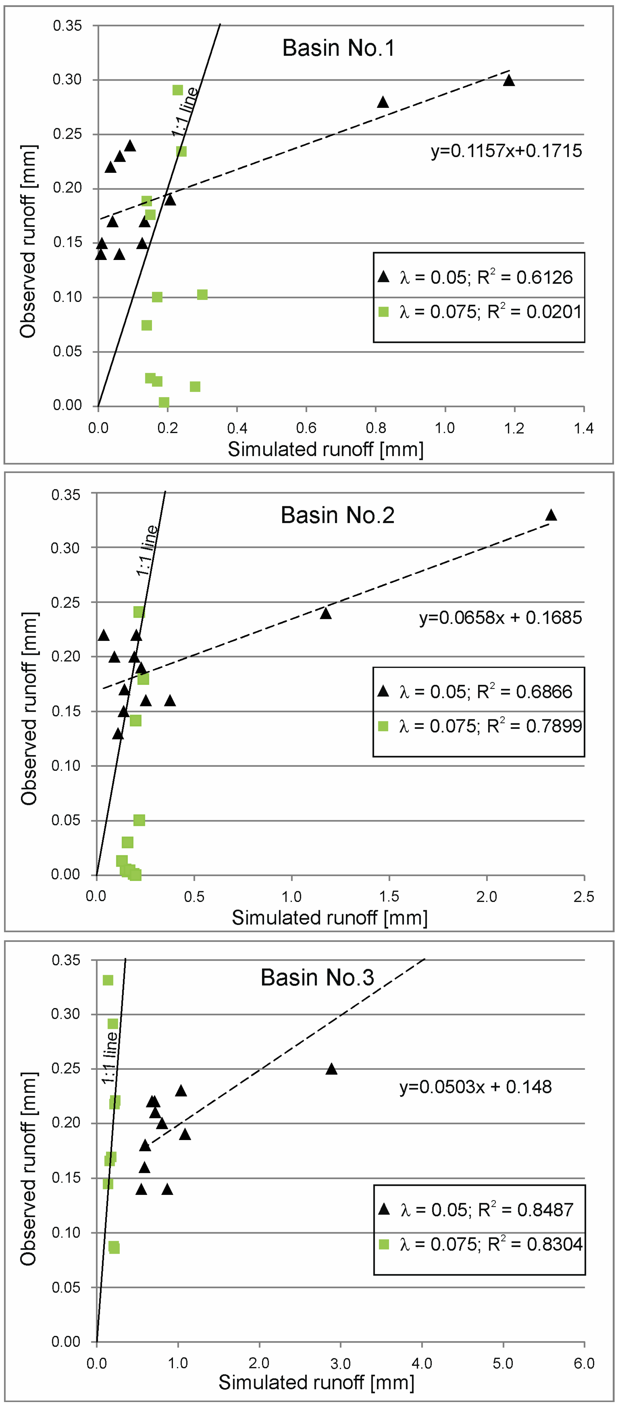
The linear regression between the measured and simulated runoff values when applying the NRCS-CN method is presented in Figure 4. For catchment 1, much better fitting of the measured and simulated runoffs (R2 = 0.61) was noted for a lower λ coefficient value of 0.05 than that for the coefficient value of 0.075. For catchment 2, the measured and modelled runoff values were better correlated than for catchment 1; but better with the λ coefficient values of 0.075 (R2 = 0.7899).
The best fit for measured and calculated runoffs was obtained for catchment 3, at a maximum value of the determination coefficient (R2 = 0.8487), corresponding to the λ coefficient value of 0.05.
In Table 3, the lag time LAG for the raised-water runoff is calculated. The selected methods included those best known, which took into account the physiographic catchment parameters independent of the meteorological conditions in the equation [36,37,38,39], and those which took into account the current water and moisture conditions [15,40,41]. The highest LAG values (19.72 h) were obtained for catchment 1 with the largest area, while the longest LAG time was obtained using Formula (11), which exceeded the value obtained from measurements (7.99 ± 2.02 h) by two and half times. Lower LAG values were obtained for catchment 3 (4.08 ± 0.83 h) and catchment 2 (2.99 ± 0.63 h), proportionally to their sizes. When using the same formula, the LAG time values for these catchments were more than three (12.88 h) and more than two (7.23 h) higher than the LAG from measurements. Considerably higher LAG values, as compared to those obtained from measurements, were also obtained when using Formula (12), yet the differences were smaller. Similarly, large discrepancies in relation to the measured LAG were noted when using Formulas (13) and (14), in which, apart from the geometrical parameters of the catchment, the quantity differentiating individual rainfall-runoff events was the average flow Q. These equations showed a high determination coefficient with the LAG measured for catchment 1 (R2 0.83). The greatest (more than three-fold) discrepancies were noted between the LAG calculated using Formula (14) and the LAG measured in relation to the largest catchment 1. The equations which included the retention parameter Si offered a better fit.
When using Formula (9) only for the largest catchment 1, the difference between the measured LAG and the calculated LAG (16.49 ± 4.65, RMSE 8.98 h) was slightly more than double. For catchment 3, the results were slightly higher (5.55 ± 1.44, RMSE 0.76 h), while for catchment 2, the method showed a good fit (2.90 ± 0.77, RMSE 0.35 h). The best fit for the measured LAG was shown by Formula (17), where the LAG for catchment 1 was the most similar (7.93 ± 1.13, RMSE 1.11 h). Moreover, similar LAG values were noted for catchment 2 (2.59 ± 0.36, RMSE of 0.52 h) and for catchment 3 (3.34 ± 0.46, RMSE of 0.87 h). Equation (17) produced the highest determination coefficient in relation to the measured LAG of all the equations (R2 0.77–0.78 h). The equations that included the constant parameter of the proportion of wetlands (W) in the catchment showed a good fit to the measured LAG. Equation (15) yielded slightly overestimated LAG values for smaller catchments, i.e., catchment 3 (5.89 h) and catchment 2 (3.84 h), and a slightly underestimated LAG for catchment 1 (6.13 h). On the other hand, Equation (16) yielded a slightly underestimated LAG for catchment 2 (2.22 h) and a comparable LAG for catchment 1 (8.74 h). The most underestimated LAG in relation to the measured LAG was obtained for Equation (10) based only on the size parameter (A).
5. Discussion
The NRCS-CN (initially SCS-CN) method, described in NEH-4 [23], was originally calibrated for small-sized (less than 8 km2) urban catchments, and has been further developed to include a wider range of conditions: from steep to flat and from heavily forested to smooth conditions. However, the method’s limitations in the universal application of its basic form are due to the fact that it was developed for estimating daily runoff from daily rainfalls without considering in detail the preceding soil moisture conditions [42]. The model ignores the effect of rainfall intensity, duration and spatial variability. For small catchments, it requires the recording of rainfall-runoff events at a high frequency. Some researchers [43] report that the runoff from catchment Q and the initial abstraction (Ia) vary according to the rainfall intensity and duration. In the event of a greater, more intense and shorter rainfall, the runoff generation time is earlier, and the infiltration is lower. The adoption of appropriate model parameters is a key research issue associated with the application of this method for forest catchments conditions [22]. Initially, in view of the NRCS-CN method having been developed based on the approximately ten-year data on the maximum annual daily total rainfalls, collected for catchments with predominant agricultural land in the temperate climate zone of the USA, for the practical application, the initial abstraction coefficient λ value was 0.2 [29,44,45]. Furthermore, in the Polish literature, the λ coefficient value was estimated according to the original method at that level [46]. However, many researchers [42,47,48,49,50] proved the great variability of the coefficient, which is determined by the local specificity of physical and geographical conditions. The coefficient is increasingly estimated at a higher or lower level. This article adopted calculation coefficient values lower than those in the original method, as higher values (λ = 0.2) implied considerably overestimated effective rainfall (Pe) values, which did not correspond to the actual runoff. Most raised-water stage episodes produced a better fit of the observed runoff value to the measured runoff value (H), at the λ coefficient values at a level of 0.05. This occurred when the rainfall P values were at a level of approximately 30 mm. At the lowest total rainfall values, the best fit corresponded to the λ coefficient of 0.075. These values were obtained by the researchers when calibrating this coefficient for other catchments [51,52,53,54,55,56].
The lag time LAG used in this study was defined as the time from the centroid of the rainfall episode to the centroid of the direct runoff. This definition was adopted as the most stable measure of the lag time. In the available literature, there are many equations to determine the LAG derived from the basic equation of the SCS method (9), in which the formula was modified mainly due to the conversion of units to or from those in the International System of Units [23,57]. This study applied the original notation of the method, as the subsequent equations yielded the same, or very similar results. Other relationships derived from the same formula, e.g., [58], are based on the CN parameter for the particular catchment linked to the maximum potential retention S with Equation (3). Consequently, they do not take into account the varying retention Si or the initial content of a certain amount of water in the catchment (AMC), thus reflecting extremely dry conditions, and the LAG values calculated using these equations are overestimated in relation to the LAG estimated on measurement (Table 3).
In the hydrographs obtained in natural catchments, some authors observe a lower LAG variability [32], while others noted non-linear relationships between the lag time, catchment area and the representative flow rate [40]. The LAG increases with an increase in the catchment area and watercourse length and decreases with an increase in the flow and slope. However, more than a twofold difference occurred because the baseflow separations used in Equation (13) produced long recessions of the direct runoff hydrographs, which consequently gave high calculated values of LAG. This Equation (13) was evaluated using these high LAG values. The lag times (LAG), when calculated by different methods, provide divergent values. The formula fitting is largely determined by the catchment size. For most equations, the catchments were selected within a broad range of sizes, from very small (less than 1 km2) to very large (several hundred km2). In that case, the equation model did not always fit small catchments. Nash [37], for the data from catchments with areas ranging from several km2 to over 2000 km2, developed a relation to estimate the LAG based on the catchment area and its average slope (11) or the watercourse length and slope (12). The greatest discrepancies between the LAG calculated and the LAG measured occurred in that case.
The most underestimated LAG in relation to the measured LAG was obtained using Equation (10) based only on the area size parameter (A). The author of Formula (10) [36] reported that the inclusion of the slope parameter did not significantly improve the predictive capability due to the high degree of correlation between the slope and the area for the study catchments. The method [41], whose Equation (17) was developed for 78 catchments with the area size most similar to that of the study catchments (0.1–14 km2), exhibited the best fit. Capece et al. [38] developed his Equation (15) on nine catchments similar to each other in terms of size (0.1–14.5 km2). That study, conducted on the basis of data from flat, afforested areas of Florida, made the LAG dependent on the catchment area (A) and the proportion of wetlands (W). The study concluded that the existing empirical relationships, used to estimate the hydrograph time parameters, generally underestimated the LAG values being observed and that the relative errors of the predicted values generally tended to increase with an increasing catchment area and a decreasing channel slope. Similarly, a fairly good fit with the LAG measured for catchment 2 and catchment 1 was obtained in Equation (16), in which the location of wetlands within the catchment was additionally significant [39].
6. Conclusions
The planning of catchments, implemented for wetland reconstruction, can bring prospective benefits through the restoration of appropriate ecosystem functions that maintain the integrity of water resources. In recent years, the processing of hydrological data using GIS techniques has become more effective and interactive, less troublesome, and often more possible, in comparison with the traditional methods, as GIS enables more efficient storage, interpretation and display of the data needed in the runoff estimation techniques in rainfall-runoff models. For the purposes of the study being the subject of a more extensive paper, a GIS-based model was developed to facilitate estimating the usefulness for planning wetland reconstruction in forest catchments. The study attempted to adapt the NRCS-CN method for the hydrological conditions prevailing in three small-sized afforested catchments. The following information was obtained as a result of adapting the NRCS-CN method to the conditions in research catchments.
The soils in the catchments under analysis are mainly of the A group. Soils in this group have low runoff potential when thoroughly wet. Water is freely transmitted through the soil. Relatively low effective rainfall values were obtained. The maximum potential retention Si value, corresponding to each pair of P-Pe events, was the effect of catchment moisture and absorptive capacity conditions. High retention capacity (expressed by the Si index) was the most pronounced for catchment 1. Selected rainfall-runoff events enabled the determination that most raised-water episodes offered a better fit between the observed and measured runoff heights (H) at the λ coefficient values at a level of 0.05, which occurred at higher total rainfalls. At lower total rainfall levels, the best fit corresponded to the λ coefficient of 0.075.
At the typical coefficient values (λ = 0.2), the initial losses exceeded the rainfall p values, and the effective rainfall Pe was not generated. The lag times LAG, calculated by different methods, provided varying values. The fitting of a particular formula was largely determined by the range of catchment size as well as the number and type of parameters considered when calibrating the model. The method based on Equation (17) showed the best fit for all catchments. Despite numerous modifications to the methods for estimating the runoff parameters, there is still a need for further refinement of critical elements of the methodology, such as the AMC procedure, the use of GIS data for data preprocessing, and the simulation of the basic quantities of an instantaneous unit hydrograph (IUH), i.e., the hydrograph peak flow up, and the runoff lag time LAG. Therefore, both the development and validation of the models and further research are necessary.
Funding
This research was Funded by the Minister of Science under “the Regional Initiative of Excellence Program”.
Data Availability Statement
The data presented in this study are available on request from the corresponding author.
Conflicts of Interest
The author declares no conflicts of interest. The funders had no role in the design of the study; in the collection, analyses, or interpretation of data; in the writing of the manuscript; or in the decision to publish the results.
References
- Salami, A.W.; Bilewu, S.O.; Ayanshola, A.M.; Oritola, S.F. Evaluation of synthetic unit hydrograph methods for the development of design storm hydrographs for Rivers in South-West, Nigeria. J. Am. Sci. 2009, 5, 23–32. [Google Scholar]
- Bhunya, P.K.; Panda, S.N.; Goel, M.K. Synthetic unit hydrograph methods: A critical review. Open Hydrol. J. 2011, 5, 1–8. [Google Scholar] [CrossRef]
- Czyzyk, K.; Mirossi, D.; Abdoulhak, A.; Hassani, S.; Niemann, J.D.; Gironás, J. Impacts of Channel Network Type on the Unit Hydrograph. Water 2020, 12, 669. [Google Scholar] [CrossRef]
- Al-Ghobari, H.; Dewidar, A.; Alataway, A. Estimation of Surface Water Runoff for a Semi-Arid Area Using RS and GIS-Based SCS-CN Method. Water 2020, 12, 1924. [Google Scholar] [CrossRef]
- Payne, J.T.; Wood, A.W.; Hamlet, A.F.; Palmer, R.N.; Lettenmeier, D.P. Mitigating the effects of climate change on the water resources of the Columbia River Basin. Clim. Change 2004, 62, 233–256. [Google Scholar] [CrossRef]
- Groves, D.G.; Yates, D.; Tebaldi, C. Developing and applying uncertain climate change projections for regional water management planning. Water Resour. Res. 2008, 44, 1–16. [Google Scholar] [CrossRef]
- Praskievicz, S.; Chang, H. A review of hydrological modelling of basin-scale climate change and urban development impacts. Prog. Phys. Geogr. Earth Environ. 2009, 33, 650–671. [Google Scholar] [CrossRef]
- Salvadore, E.; Bronders, J.; Batelaan, O. Hydrological modelling of urbanized catchments: A review and future directions. J. Hydrol. 2015, 529, 62–81. [Google Scholar] [CrossRef]
- Sishodia, R.P.; Shukla, S.; Wani, S.P.; Graham, W.D.; Jones, J.W. Future irrigation expansion outweigh groundwater recharge gains from climate change in semi-arid India. Sci. Total Environ. 2018, 635, 725–740. [Google Scholar] [CrossRef]
- Gupta, P.K.; Panigrahy, S.; Parihar, J.S. Impact of climate change on runoff of the major river basins of India using global circulation model (HadCM3) projected data. J. Indian Soc. Remote Sens. 2011, 39, 337–344. [Google Scholar] [CrossRef]
- Kuczera, G.; Kavetski, D.; Franks, S.; Thyer, M. Towards a Bayesian total error analysis of conceptual rainfall-runoff models: Characterising model error using storm-dependent parameters. J. Hydrol. 2006, 331, 161–177. [Google Scholar] [CrossRef]
- Grzebinoga, M.; Walega, A. Wpływ struktury sieci rzecznej na parametry wezbrań określone z modelu GUIH. Monogr. KGW PAN 2014, 1, 341–352. [Google Scholar]
- Vansteenkiste, T.; Tavakoli, M.; Ntegeka, V.; De Smedt, F.; Batelaan, O.; Pereira, F.; Willems, P. Intercomparison of hydrological model structures and calibration approaches in climate scenario impact projections. J. Hydrol. 2014, 519, 743–755. [Google Scholar] [CrossRef]
- Banasik, K.; Wałęga, A.; Węglarczyk, S.; Więzik, B. Update of the Methodology for Calculating Maximum Flow and Precipitation with a Specified Probability of Exceedance for Controlled and Uncontrolled Catchments, as well as Identification of Precipitation-to-Runoff Transformation Models; KZGW: Warsaw, Poland, 2017; p. 137. [Google Scholar]
- USDA-SCS. NEH. Use of Storm and Watershed Characteristics in Synthetic Hydrograph Analysis and Application; USDA: Washington, DC, USA, 1957.
- USDA-NRCS. Urban Hydrology for Small Watershed; TR55; USDA: Washington, DC, USA, 2021.
- Mishra, S.K.; Singh, V.P. SCS-CN Method. Part I: Derivation of SCS-CN-Based Models. Acta Geophys. Pol. 2002, 50, 457–477. [Google Scholar]
- Chow, V.T.; Maidment, D.K.; Mays, L.W. Applied Hydrology; McGrow-Hill: New York, NY, USA, 1988; p. 565. [Google Scholar]
- ASCE. Curve Number Hydrology: State of the Practice; Hawkins, R.H., Ward, T.J., Woodward, D.E., van Mullem, J.A., Eds.; American Society of Civil Engineers: Reston, VA, USA, 2009. [Google Scholar]
- Wałęga, A.; Drożdżal, E.; Piórecki, M.; Radoń, R. Wybrane problemy związane z modelowaniem odpływu ze zlewni niekontrowanych w aspekcie projektowania stref zagrożenia powodziowego. Acta Sci. Pol. Form. Circumiectus 2012, 11, 57–68. [Google Scholar]
- Krzanowski, S.; Miler, A.T.; Wałęga, A. Wpływ warunków wilgotnościowych na estymację wartości parametru CN w zlewni górskiej. Infrastr. Ekol. Teren. Wiejs. 2013, 3–4, 105–117. [Google Scholar]
- Miler, A.; Okoński, B. Possibilities of modeling flood runoff from wetlands of the Rychtalskie Forest Promotional Forest Complex. Zesz. Nauk. Wydz. Bud. Inż. Środ. Pol. Koszal. 2016; 528, 717–728. [Google Scholar]
- USDA-SCS. NEH, Section 4: Hydrology; USDA: Washington, DC, USA, 1985.
- Strapazan, C.; Irimuș, I.-A.; Șerban, G.; Man, T.C.; Sassebes, L. Determination of Runoff Curve Numbers for the Growing Season Based on the Rainfall–Runoff Relationship from Small Watersheds in the Middle Mountainous Area of Romania. Water 2023, 15, 1452. [Google Scholar] [CrossRef]
- Sahu, R.K.; Mishra, S.K.; Eldho, T.I.; Jain, M.K. An advanced soil moisture accounting procedure for SCS curve number method. Hydrol. Process. 2007, 21, 2827–2881. [Google Scholar] [CrossRef]
- USDA-NRCS. NEH, Part 630, Hydrology; USDA: Washington, DC, USA, 2009.
- Banasik, K.; Ignar, S. Determination of effective rainfall using the SCS method based on measured precipitation and runoff. Przegl. Geofiz. 1983, 3–4, 409–414. [Google Scholar]
- Hawkins, R.H.; Hjelmfelt, A.T., Jr.; Zevenbergen, A.W. Runoff probability, storm depth and curve numbers. J. Irrig. Drain Eng. 1985, 111, 330–340. [Google Scholar] [CrossRef]
- Garg, V.; Nikam, B.; Thakur, P.; Aggarwal, S. Assessment of the effect of slope on runoff potential of a watershed using NRCS-CN Method. Int. J. Hydrol. Sci. Technol. 2013, 3, 141–159. [Google Scholar] [CrossRef]
- Nash, J.E. The form of instantaneous unit hydrograph. Surf. Water Previs. Evaporation. Int. Assoc. Sci. Hydrol. Publ. 1957, 45, 114–121. [Google Scholar]
- Lee, Y.H.; Singh, V.P. Application of the Kalman Filter to the Nash Model. Hydrol. Process. 1998, 12, 755–767. [Google Scholar] [CrossRef]
- Karabova, B.; Sikorska, A.; Banasik, K.; Kohnova, S. Parameters determination of a conceptual rainfall-runoff model for a small catchment in Carpathians. Ann. Wars. Univ. Life Sci.-SGGW Land Reclam. 2012, 44, 155–162. [Google Scholar] [CrossRef]
- Yan, B.; Guo, S.; Liang, J.; Sun, H. The generalized Nash model for river flow routing. J. Hydrol. 2015, 530, 79–86. [Google Scholar] [CrossRef]
- Overton, D.E.; Meadows, M.E. History of Parametric Stormwater Modeling. In Stormwater Modeling; Academic Press: New York, NY, USA, 1976. [Google Scholar]
- Monajemi, P.; Khaleghi, S.; Maleki, S. Derivation of instantaneous unit hydrographs using linear reservoir models. Hydrol. Res. 2021, 52, 339–355. [Google Scholar] [CrossRef]
- Sheridan, J.M. Hydrograph time parameters for flatland watersheds. Trans. ASAE 1994, 37, 103–113. [Google Scholar] [CrossRef]
- Nash, J.E. A Unit Hydrograph Study, with Particular Reference to British Catchments. Proc. Inst. Civ. Eng. 1960, 17, 249–282. [Google Scholar] [CrossRef]
- Capece, J.C.; Campbell, K.L.; Baldwin, L.B. Estimating runoff peak rates from flat, high-water-table watersheds. Trans. ASAE 1988, 31, 74–81. [Google Scholar] [CrossRef]
- Kennedy, R.J.; Watt, W.E. The relationship between lag time and the physical characteristics of drainage basins in Southern Ontario. IAHS Publ. 1967, 85, 866–874. [Google Scholar]
- Askew, A.J. Variation in lag time for natural catchments. J. Hydraul. Div. 1970, 96, 317–330. [Google Scholar] [CrossRef]
- Simas, M.J.; Hawkins, R.H. Lag Time characteristics for Small Watersheds in the U.S. In Proceedings of the Second Federal Interagency Hydrologic Modeling Conference, Las Vegas, CA, USA, July 28–August 1 2002; ASCE: Las Vegas, NV, USA, 2002. [Google Scholar]
- Verma, S.R.; Verma, K.S.; Mishra, K.; Singh, A.; Jayaraj, G.K. A revisit of NRCS-CN inspired models coupled with RS and GIS for runoff estimation. Hydrol. Sci. J. 2017, 62, 1891–1930. [Google Scholar] [CrossRef]
- Wang, X.; Bi, H. The Effects of Rainfall Intensities and Duration on SCS-CN Model Parameters under Simulated Rainfall. Water 2020, 12, 1595. [Google Scholar] [CrossRef]
- Tirkey, A.S.; Pandey, A.C.; Nathawat, M.S. Use of high-resolution satellite data, GIS and NRCS-CN technique for the estimation of rainfall-induced run-off in small catchment of Jharkhand India. Geocarto. Int. 2013, 29, 778–791. [Google Scholar] [CrossRef]
- Vojtek, M.; Vojteková, J. Land use change and its impact on surface runoff from small basins: A case of Radiša basin. Folia Geogr. 2019, 61, 104–125. [Google Scholar]
- Zyzdroń, T.; Wałęga, A.; Bochenek, W. Zastosowanie wybranych modeli hydrologicznych do określania wielkości spływu powierzchniowego. Acta Sci. Pol. Form. Circumiectus 2014, 13, 81–93. [Google Scholar]
- Golding, B.L. Discussion of runoff curve number with varying site moisture. J. Irrig. Drain. Div. 1979, 105, 441–442. [Google Scholar] [CrossRef]
- Mishra, S.K.; Singh, V.P. Soil Conservation Service Curve Number (SCS-CN) Methodology; Kluwer Academic Publishers: Dordrecht, The Netherlands, 2013. [Google Scholar]
- Verma, S.; Singh, A. Efficacy of slope-adjusted curve number models with varying initial abstraction coefficient for runoff estimation. Int. J. Hydrol. Sci. Technol. 2018, 8, 317–338. [Google Scholar] [CrossRef]
- Soulis, K. Soil Conservation Service Curve Number (SCS-CN) Method: Current Applications, Remaining Challenges, and Future Perspectives. Water 2021, 13, 192. [Google Scholar] [CrossRef]
- Woodward, D.E.; Hawkins, R.H.; Jiang, R.; Hjelmfelt, J.; Allen, T.; Van Mullem, J.A.; Quan, Q.D. Runoff curve number method: Examination of the initial abstraction ratio. In Proceedings of the World Water & Environmental Resources Congress 2003, Philadelphia, PA, USA, 23–26 June 2003; pp. 1–10. [Google Scholar]
- Lamont, S.J.; Eli, R.N.; Fletcher, J.J. Continuous hydrologic models and curve numbers: A Path Forward. J. Hydrol. Eng. 2008, 13, 621–635. [Google Scholar] [CrossRef]
- Wang, X.; Shang, S.; Yang, W.; Melesse, A.M. Simulation of an agricultural watershed using an improved curve number method in SWAT. Am. Soc. Agric. Biol. Eng. 2008, 51, 1323–1339. [Google Scholar] [CrossRef]
- Fu, S.; Zhang, G.; Wang, N.; Luo, L. Initial Abstraction Ratio in the SCS-CN Method in the Loess Plateau of China. Trans. Am. Soc. Agric. Biol. Eng. 2011, 54, 163–169. [Google Scholar]
- Zhou, S.M.; Lei, T.W. Calibration of SCS-CN initial abstraction ratio of a typical small watershed in the Loess Hilly-Gully region. China Agric. Sci. 2011, 44, 4240–4247. [Google Scholar]
- Noori, N. Effects of initial abstraction ratio in SCS-CN method on modeling the impacts of urbanization on peak flows. In Proceedings of the World Environmental and Water Resources Congress 2012: Crossing Boundaries, Albuquerque, NM, USA, 20–24 May 2012; ASCE: Albuquerque, NM, USA, 2012; pp. 329–338. [Google Scholar]
- USDA-SCS. NEH, Part 630 Hydrology, Chapter 14 Stage Discharge Relations (Draft); USDA: Washington, DC, USA, 2010.
- DHI. MIKE 11—A Modeling System for Rivers and Channels—Reference Manual; Danish Hydraulic Institute: Hørsholm, Danmark, 2009. [Google Scholar]
Figure 1.
The location of 3 experimental catchments and meteorological stations in Regional Directorate of State Forests of Olsztyn and Forestry Department of Spychowo.
Figure 1.
The location of 3 experimental catchments and meteorological stations in Regional Directorate of State Forests of Olsztyn and Forestry Department of Spychowo.

Figure 2.
DEM of the three studied catchments.

Figure 3.
A view on the rainfall-runoff process formation (modified by the author).

Figure 4.
A comparison between the measured and predicted runoff depths for surveyed catchments.


Table 1.
Characteristics of the study catchments.
| Characteristic | Catchment | ||
|---|---|---|---|
| 1 | 2 | 3 | |
| Catchment area A (ha) | 747 | 67.6 | 167 |
| Catchment use: forest habitats as the percentages of the catchment area; types of dominant tree species (age) 1 | BMw 52.8%; So-Sw (65) BMsw 18%; Sw-So (50) Bsw 15%; So (50) B 6%; Ol (45) Ol 5%; Ol (100) BMb 1.7%; Brzo-So (50) LMb 1.5%; Ol-Brz (40) | Bsw 41.7%; So (65) BMsw 25%; So-Sw (90) BMw 16.5%; Sw-So-Brz (45) Ol 9.8%; Ol (45) Bw 1.6%; Brz (80) | R 31.7% LMsw 21.2%; So (55) BMsw 11.5%; So (60) BMw 8.6%; Brz-Sw (55.30) LMw 6.3%; So (110) Bsw 3.2%; So (120) B 7.1%; Brz (50) BMb 4.1%; So (155) LMb 2.5%; Brz-Ol (60) Bb 2.1%; So (25) Ol 1.7%; Ol-Brz (55) |
| Soil types 2 | Bgw, Bw, RDb, Tn, Mt1, Tp | RDbr, RDw, Bgw, Mt1, Bgts | RDbr, RDb, Bgw, Tw, Mt1, Gt |
| Granulometry groups of soils | S, LS | S | S |
| CNII | 38 | 52 | 45.8 |
| CNI | 21.2 | 32.2 | 27 |
| Average catchment slope, ‰ | 0.88 | 2.25 | 0.81 |
| Range of altitude H (m a.s.l.) | 136.5–134.1 | 123.1–121.25 | 135.15–134.1 |
| Length of watercourse [m] | 4380 | 1060 | 1450 |
| Density of hydrographic network G [km·km−2] | 3.36 | 1.30 | 1.93 |
| Watercourse slope [‰] | 0.548 | 1.745 | 0.724 |
Note: 1 BMw—Moist mixed coniferous forest, BMsw—Fresh mixed coniferous forest, Bsw—Fresh coniferous forest, B—Bog, Ol—alder forest, BMb-Boggy mixed coniferous forest, LMb—Boggy mixed forest, Bw—Moist coniferous forest, R—rural, LMsw—Fresh mixed broadleaved forest, LMw—Moist mixed broadleaved forest, Bb—Bog coniferous fores; So—Pine, Sw—Spruce, Ol—Alder, Brz—Birch; 2 S—sand, LS—loamy sand; Bgw—gley and podzolic soils, Bw—podzolic soils, RDb—rusty podzolic soils, Tn—peaty soils of low moors, Mt1—murshic soil, Tp—transitional moor soil, RDbr—rusty brown soils, RDw—rusty soil, Bgts—gley and podzolic peaty soil, Tw—peaty soil of raised bog, Gt—gley-peat soil.
Table 2.
Rainfall-runoff event parameters in the studied catchments.
| Rainfall-Runoff Event No | AMC | Catchment 1 | Catchment 2 | Catchment 3 | |||||||||||||||
|---|---|---|---|---|---|---|---|---|---|---|---|---|---|---|---|---|---|---|---|
| P | Pe | α | Si | H | q | P | Pe | α | Si | H | q | P | Pe | α | Si | H | q | ||
| 1 | II | 31.2 | 0.21 | 0.66 | 129.6 | 0.19 | 2.20 | 24.9 | 0.23 | 0.92 | 99.9 | 0.19 | 2.20 | 25.1 | 0.81 | 3.20 | 82.8 | 0.20 | 2.31 |
| 2 | II | 23.8 | 0.01 | 0.05 | 113.4 | 0.15 | 1.74 | 25.3 | 0.25 | 1.00 | 100.8 | 0.16 | 1.85 | 25.7 | 0.87 | 3.38 | 83.6 | 0.14 | 1.62 |
| 3 | I | 78.2 | 0.82 | 1.05 | 309.2 | 0.28 | 3.24 | 66.9 | 1.18 | 1.76 | 246.4 | 0.24 | 2.78 | 65.7 | 2.89 | 4.40 | 200.6 | 0.25 | 2.89 |
| 4 | II | 25.9 | 0.04 | 0.16 | 118.3 | 0.17 | 1.97 | 27.4 | 0.38 | 1.37 | 104.6 | 0.16 | 1.85 | 27.5 | 1.09 | 3.96 | 86.1 | 0.19 | 2.20 |
| 5 | II | 29.3 | 0.13 | 0.46 | 125.7 | 0.17 | 1.97 | 22.9 | 0.14 | 0.61 | 96.1 | 0.15 | 1.74 | 23.1 | 0.59 | 2.55 | 79.7 | 0.16 | 1.85 |
| 6 | II | 23.5 | 0.01 | 0.03 | 112.7 | 0.14 | 1.62 | 22.2 | 0.11 | 0.50 | 94.5 | 0.13 | 1.50 | 22.7 | 0.55 | 2.43 | 79.0 | 0.14 | 1.62 |
| 7 | I | 84.1 | 1.18 | 1.41 | 320.1 | 0.30 | 3.24 | 79.5 | 2.33 | 2.93 | 266.9 | 0.33 | 3.36 | 82.4 | 5.64 | 6.84 | 220.9 | 0.45 | 3.47 |
| 8 | II | 26.8 | 0.06 | 0.23 | 120.3 | 0.14 | 1.62 | 23.0 | 0.14 | 0.62 | 96.3 | 0.17 | 1.97 | 23.2 | 0.60 | 2.58 | 79.8 | 0.18 | 2.08 |
| 9 | I | 55.3 | 0.04 | 0.07 | 261.1 | 0.22 | 2.66 | 42.1 | 0.04 | 0.09 | 196.9 | 0.22 | 2.55 | 45.2 | 0.71 | 1.58 | 169.2 | 0.22 | 2.55 |
| 10 | II | 29.1 | 0.13 | 0.44 | 125.2 | 0.15 | 1.74 | 24.2 | 0.19 | 0.80 | 98.5 | 0.20 | 2.31 | 24.0 | 0.68 | 2.84 | 81.1 | 0.22 | 2.55 |
| 11 | I | 58.9 | 0.09 | 0.16 | 269.4 | 0.24 | 2.78 | 49.2 | 0.20 | 0.41 | 212.8 | 0.22 | 2.55 | 49.3 | 1.04 | 2.10 | 176.3 | 0.23 | 2.66 |
| 12 | I | 57.2 | 0.06 | 0.11 | 265.5 | 0.23 | 2.66 | 45.2 | 0.09 | 0.20 | 203.9 | 0.20 | 2.31 | 45.3 | 0.72 | 1.59 | 169.4 | 0.21 | 2.43 |
Note: P—total rainfall (mm); Pe—effective rainfall (mm); α—runoff coefficient (%); Si—maximum potential retention (mm); H—runoff (mm); q—runoff [dm3·s−1·km−2]. AMC—Antecedent Soil Moisture Condition [%].
Table 3.
A comparison of runoff lag times (LAG) for the analysed catchments, determined based on measurements and empirical equations. Denotations: W, wetland percent (%); I, main channel slope (%); i, main channel slope (m/m); Y, average catchment slope (%); l, length of channel from headwater to outlet (km); Si, maximum potential retention calculated from the CN for rainfall-runoff event (mm); B, catchment width (m); L, maximum distance of flow length (m); A—drainage area (km2); Q—runoff volume dm3·s−1; R2, Determination coefficient (added when possible variance of formula components); RMSE—root mean square error (added when possible variance of formula components).
| Author of the Method | Formula for LAG Estimation | Catchment 1 | Catchment 2 | Catchment 3 | |
|---|---|---|---|---|---|
| Equation No | Lag (h) Mean ± SD R2 RMSE | Lag (h) Mean ± SD R2 RMSE | Lag (h) Mean ± SD R2 RMSE | ||
| USDA-SCS [1957] | (9) | 16.49 ± 4.65 0.75 8.98 | 2.90 ± 0.77 0.79 0.35 | 5.55 ± 1.44 0.76 1.66 | |
| Sheridan [1994] | (10) | 3.51 | 0.83 | 1.43 | |
| Nash 1 [1960] | (11) | 19.72 | 7.23 | 12.88 | |
| Nash 2 [1960] | (12) | 15.37 | 6.85 | 10.06 | |
| Askew 1 [1970] | (13) | 17.16 ± 1.02 0.83 9.6 | 7.59 ± 0.39 0.51 4.69 | 10.22 ± 0.54 0.65 6.26 | |
| Askew 2 [1970] | (14) | 18.0 ± 1.07 0.83 10.41 | 7.36 ± 0.38 0.51 4.46 | 11.35 ± 0.60 0.65 7.38 | |
| Capece et al. [1988] | (15) | 6.13 | 3.84 | 5.89 | |
| Kennedy; Watt [1967] | (16) | 8.74 | 2.22 | 7.88 | |
| Simas et al. [2002] | (17) | 7.93 ± 1.13 0.77 1.11 | 2.59 ± 0.36 0.78 0.52 | 3.34 ± 0.46 0.77 0.87 | |
| Estimated on measurement | 7.99 ± 2.02 | 2.99 ± 0.63 | 4.08 ± 0.83 |
Disclaimer/Publisher’s Note: The statements, opinions and data contained in all publications are solely those of the individual author(s) and contributor(s) and not of MDPI and/or the editor(s). MDPI and/or the editor(s) disclaim responsibility for any injury to people or property resulting from any ideas, methods, instructions or products referred to in the content. |
© 2024 by the author. Licensee MDPI, Basel, Switzerland. This article is an open access article distributed under the terms and conditions of the Creative Commons Attribution (CC BY) license (https://creativecommons.org/licenses/by/4.0/).
Share and Cite
MDPI and ACS Style
Kobus, S. Rainfall-Runoff Parameter Estimation from Ungauged Flat Afforested Catchments Using the NRCS-CN Method. Water 2024, 16, 1247. https://0-doi-org.brum.beds.ac.uk/10.3390/w16091247
AMA Style
Kobus S. Rainfall-Runoff Parameter Estimation from Ungauged Flat Afforested Catchments Using the NRCS-CN Method. Water. 2024; 16(9):1247. https://0-doi-org.brum.beds.ac.uk/10.3390/w16091247
Chicago/Turabian StyleKobus, Szymon. 2024. "Rainfall-Runoff Parameter Estimation from Ungauged Flat Afforested Catchments Using the NRCS-CN Method" Water 16, no. 9: 1247. https://0-doi-org.brum.beds.ac.uk/10.3390/w16091247
Note that from the first issue of 2016, this journal uses article numbers instead of page numbers. See further details here.