
Carrier-Free Ultra-Wideband Sensor Target Recognition in the Jungle Environment
by
Jianchao Li
1,
Shuning Zhang
1,*,
Lingzhi Zhu
1,2,
Si Chen
1,
Linsheng Hou
1,
Xiaoxiong Li
1 and
Kuiyu Chen
1,3 1
School of Electronic and Optical Engineering, Nanjing University of Science and Technology, Nanjing 210094, China
2
College of Electronic and Information Engineering, Nanjing University of Aeronautics and Astronautics, Nanjing 210016, China
3
College of Electronic and Optical Engineering, Nanjing University of Posts and Telecommunications, Nanjing 210003, China
*
Author to whom correspondence should be addressed.
Remote Sens. 2024, 16(9), 1549; https://0-doi-org.brum.beds.ac.uk/10.3390/rs16091549
Submission received: 11 March 2024
/
Revised: 18 April 2024
/
Accepted: 19 April 2024
/
Published: 26 April 2024
(This article belongs to the Topic Radar Signal and Data Processing with Applications)
Abstract
:Carrier-free ultra-wideband sensors have high penetrability anti-jamming solid ability, which is not easily affected by the external environment, such as weather. Also, it has good performance in the complex jungle environment. In this paper, we propose a jungle vehicle identification system based on a carrier-free ultra-wideband sensor. Firstly, a composite jungle environment with the target vehicle is modeled. From this model, the simulation obtains time-domain echoes under the excitation of carrier-free ultra-wideband sensor signals in different orientations. Secondly, the time-domain signals are transformed into MTF images through the Markov transfer field to show the statistical characteristics of the time-domain echoes. At the same time, we propose an improved RepVGG network. The structure of the RepVGG network contains five stages, which consist of several RepVGG Blocks. Each RepVGG Block is created by combining convolutional kernels of different sizes using a weighted sum. We add the self-attention module to the output of stage 0 to improve the ability to extract the features of the MTF map and better capture the complex relationship between characteristics during training. In addition, a self-attention module is added before the linear layer classification output in stage 4 to improve the classification accuracy of the network. Moreover, a combined cross-entropy loss and sparsity penalty loss function helps enhance the performance and accuracy of the network. The experimental results show that the system can recognize jungle vehicle targets well.
1. Introduction
Sensor target recognition in jungle environments is of great significance and has a wide range of applications in forest protection, jungle rescue, and jungle intrusion alarms. However, in jungle environments, foliage shading, propagation attenuation, and temperature variations make it extremely difficult for conventional optical and infrared sensors to detect targets. However, carrier-free UWB sensors can compensate for these shortcomings because of their advantages such as high strong anti-interference capability [1], distance resolution [2], low power consumption [3], good electromagnetic penetration [4], and insensitivity to light and climate factors. Carrier-free UWB sensors have been widely used in some fields, such as human movement recognition [5], ground-penetrating mining [6], micro-Doppler [7], medical diagnosis [8], underwater detection [9], SAR imaging [10], network communications [11], and navigation [12]. Existing carrier-free UWB sensor target recognition is mainly applied to human movement recognition and gesture recognition. There is little research on large-size complex targets using carrier-free UWB sensors in jungle environments. This paper uses a carrier-free UWB sensor to identify jungle environment vehicle targets to help in jungle rescue and other applications.
UWB sensors have high-resolution characteristics [13], and the echo in the one-dimensional time domain is similar to those of the HRRP (high-resolution range profile). Many researchers have launched studies on HRRP target recognition using machine learning methods, such as Extreme Value Distribution [14], continuous learning based on CVAE-GAN [15], methods for CNN with Multi-Axis Attention and Residual Connections [16], a temporal–spatial feature aggregation network (TSFA-Net) [17], Composite Deep Networks [18], and Attention-ERTCN [19]. Although HRRP is processed in the frequency domain and carrier-free UWB sensor echoes are processed in the time domain, despite the difference in the processing of data, the methods of identification can be learned from each other. For target recognition in carrier-free UWB sensors, many researchers have proposed recognition methods for different tasks, such as semi-supervised stacked convolutional denoising autoencoder (SCDAE) [20], Deep Residual Shrinkage Learning [21], and Multi-Task Self-Supervised Learning [22]. All the above methods are for the identification of one-dimensional time-domain echoes. With the development of deep learning, more and more researchers have drawn on the application of deep learning in the image field, applying deep learning to feature extraction and recognition, unlike traditional signal processing, where features are extracted manually. The use of the one-dimensional signal to two-dimensional image transformation for classification, fault diagnosis, and medical diagnosis has attracted more and more researchers. For example, a coal–rock interface recognition method based on Gramian Angular Field (GAF)-deep learning is proposed to identify coal–rock interfaces [23]. Chengang Lyu proposes a method based on the Gramian Angular Field (GAF) and a convolutional neural network (CNN) [24]. Signal intra-pulse sequences are transformed into gray-scaled STFT spectrograms, and a CNN network is designed to extract features and classify the spectrogram [25]. Kah Liang Ong proposes a speech emotion recognition method that combines the Mel spectrogram with the Short-Term Fourier Transform (Mel-STFT) and Improved Multiscale Vision Transformers (MViTv2) [26]. However, Markov transfer field images possess several advantages in comparison with time–frequency maps and GAF transformations. Firstly, they excel in representing the local features of the signal. Secondly, they are superior in capturing the time-series relationship of the signal. Additionally, they offer better interpretability and require less computational effort. Therefore, we use a Markov transfer field to convert the echoes from the one-dimensional time domain of the carrier-free UWB sensor into a two-dimensional Markov transfer field map.
The concept of the self-attention mechanism was initially introduced in the year 2017, primarily for the purpose of processing information in text form [27]. After that, the self-attention module expanded into other fields, such as image classification [28] and semantic segmentation [29]. Self-attention module-based methods are capable of capturing the interrelationships and dependencies among image pixels, thereby enhancing the precision of semantic segmentation [30]. Adopting a self-attention structure minimizes the dependence on manually tuned parameters, grasps the intrinsic correlations among features, and augments the network model’s interpretability [31]. The self-attention module is effective at forming global interdependencies among features [32]. The self-attention module enables the model to focus more on the critical information within the text [33]. The self-attention module facilitates adaptive concentration on various regions and the capture of features [34]. Therefore, in this paper, for the task of carrier-free UWB sensor target identification, we embedded the self-attention module into the RepVGG network. It can help the network extract the features of the images better, improve classification accuracy, and make the model have good generalization. At the same time, combining the advantages of simplicity of structure, efficient running speed, and good performance of RepVGG [35], it has good performance for the task of target recognition in the jungle, which is very suitable for application scenarios such as jungle rescue and forest intrusion alarms.
In this paper, an improved RepVGG network is proposed to improve the ability to extract features from the MTF graph by adding a self-attention module to the output of stage 0, which helps the network to better capture the complex relationship among the features. Another self-attention module is incorporated before the output of the linear layer classification in stage 4 during training to improve the classification accuracy of the network. In addition, a loss function combining cross-entropy loss and sparsity penalty is proposed to enhance the performance and accuracy of the network. The experimental results show that the network can identify jungle vehicle targets well. The main contributions of this paper are summarized as follows:
- (1)
- We propose an enhanced scheme for identifying a target sensor on carrier-free UWB jungle vehicles and model four types of vehicle targets in the jungle composite electromagnetic environment for a carrier-free UWB sensor.
- (2)
- We use the MTF Markov transfer field method to convert a one-dimensional echo signal into a two-dimensional image, which can reflect the internal dynamics and correlations in the signal and improve the accuracy and robustness of image classification.
- (3)
- An improved REPVGG network is proposed with two areas of improvement. Firstly, the self-attention module is embedded in stage 0 and stage 4. The self-attention module in stage 0 can help the network to extract more integral features. In stage 4, the network embedded in the self-attention module can better adapt to the variability in different input image features and has better generalization performance. Secondly, we combine the sparsemax loss and cross-entropy loss functions to improve the classification accuracy.
This paper continues as follows: Section 2 provides a concise overview of the electromagnetic modeling of vehicle targets in the jungle environment by a carrier-free UWB sensor and the conversion of the one-dimensional time-domain echoes into two-dimensional images by MTF Markov transfer field. Section 3 describes the details of the improved RepVGG network. Section 4 presents the simulation results and comparative analysis. Section 5 covers the conclusions and discussion of future work.
2. Related Works
2.1. Carrier-Free Ultra-WideBand Sensor
An ultra-wideband signal is defined as a signal with a relative bandwidth greater than 25%, i.e.,
where and refer to the highest frequency and lowest frequency defined by the power spectrum of the ultra-wideband signal at around −20 dB from the peak. A carrier-free ultra-wideband sensor transmits narrow nanosecond pulses in the time domain without a carrier frequency, which can be classified into three categories according to waveforms as follows: unipolar pulses, mono, and multicircular waves. Theoretically, the transmit signal of a carrier-free ultra-wideband sensor resembles a Dirac function. In practice, we usually do not have access to infinitely short time or spatial intervals to describe an instantaneous shock or signal like a Dirac function. Gaussian functions have a finite width and are therefore more suitable for describing phenomena in a finite time or space range. Meanwhile, sensors, circuits, or instruments in real physical systems often have limited response time or bandwidth. This means that they cannot accurately detect or process transient shock signals. The actual response of these systems can be better modeled by using Gaussian functions. Consequently, in practical application, we approximate the Dirac function by a Gaussian function. In other words, the carrier-free UWB signals can be equated with a Gaussian function:
where is the peak value of the emitted signal. is the pulse width factor that satisfies the equation: , where is the equivalent pulse width of the instantaneous pulse. is the delay of the peak value. When , the pulse signal reaches peak amplitude.
According to the theory of transient electromagnetic scattering, the impulse response of any target consists of the following two parts: the impulse component generated by the target’s discontinuous boundary (early response) and the radiation component formed by the target’s induced current at the natural frequency point (late response). The early response of the target is generated by the interaction of the incident signal wavefront with the target, reflecting the local characteristics of the object, and is manifested in the time domain as a series of wavefronts corresponding to different scattering centers. The amplitude of the resonance component of the late response and the propagation component of the signal at the scattering centers are weak. So, ideally, we ignore the late response of the target, and we also ignore the propagation effect of the signal among the various scattering centers of the complex target, considering the complex target as consisting of a single independent scattering center, and these independent scattering centers as ideal point targets, and only considering the time delay of the echo signal and the amplitude attenuation, simplified into the following equation:
where is the number of strong scattering points. is the amplitude of each scattering center. is the time delay of the radial distance from the radar for each scattering center. is used to describe the attitude angle of the target, and is the phase shift corresponding to each scattering center.
2.2. Modeling the Electromagnetic Environment of Jungle Vehicle Targets
We use the forest scattering model MIMICS proposed by F.T. Ulaby, who works at the Wave Scattering Research Centre at the University of Michigan, USA. The MIMICS model has been commonly used in the study of electromagnetic scattering properties of forest vegetation. The vegetation model was divided into three layers from bottom to top as follows: a ground layer at the bottom, a trunk layer in the middle, and a canopy layer at the top. The layers of the model and the composition of the layers are shown in Table 1.
The tree model in this paper is shown in Figure 1. The 3D modeling of the tree is carried out in simulation software, which includes the canopy layer, the trunk layer, and the ground layer in order from top to bottom. The top canopy layer consists of leaves and branches, where the leaves are modeled by using arbitrarily oriented media elliptic discs. The trunk layer is modeled by using a relatively large dielectric disc placed perpendicular to the ground. The ground layer is the media plane generated by the Gaussian roughness surface and is placed at the bottom of the model.
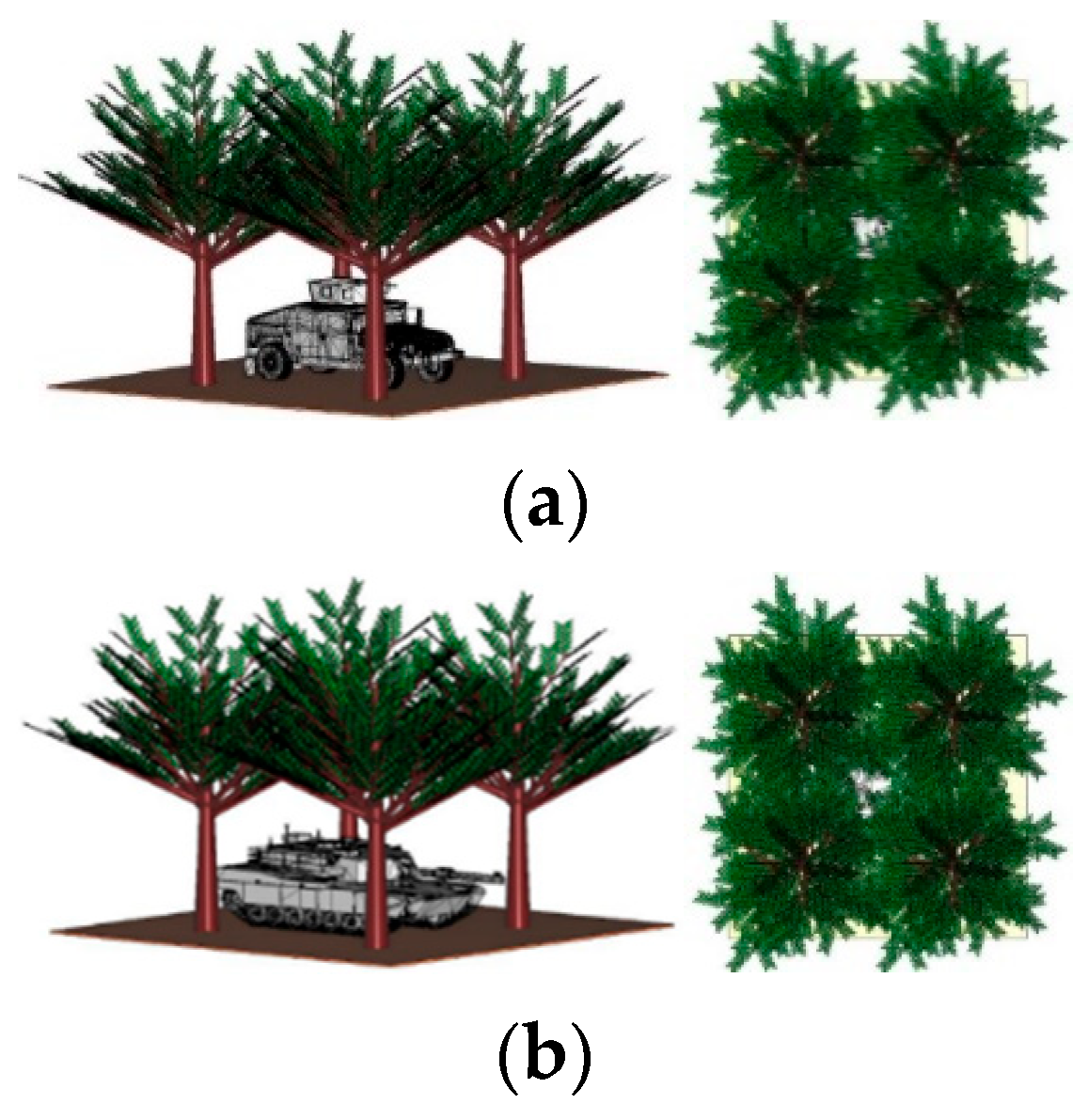
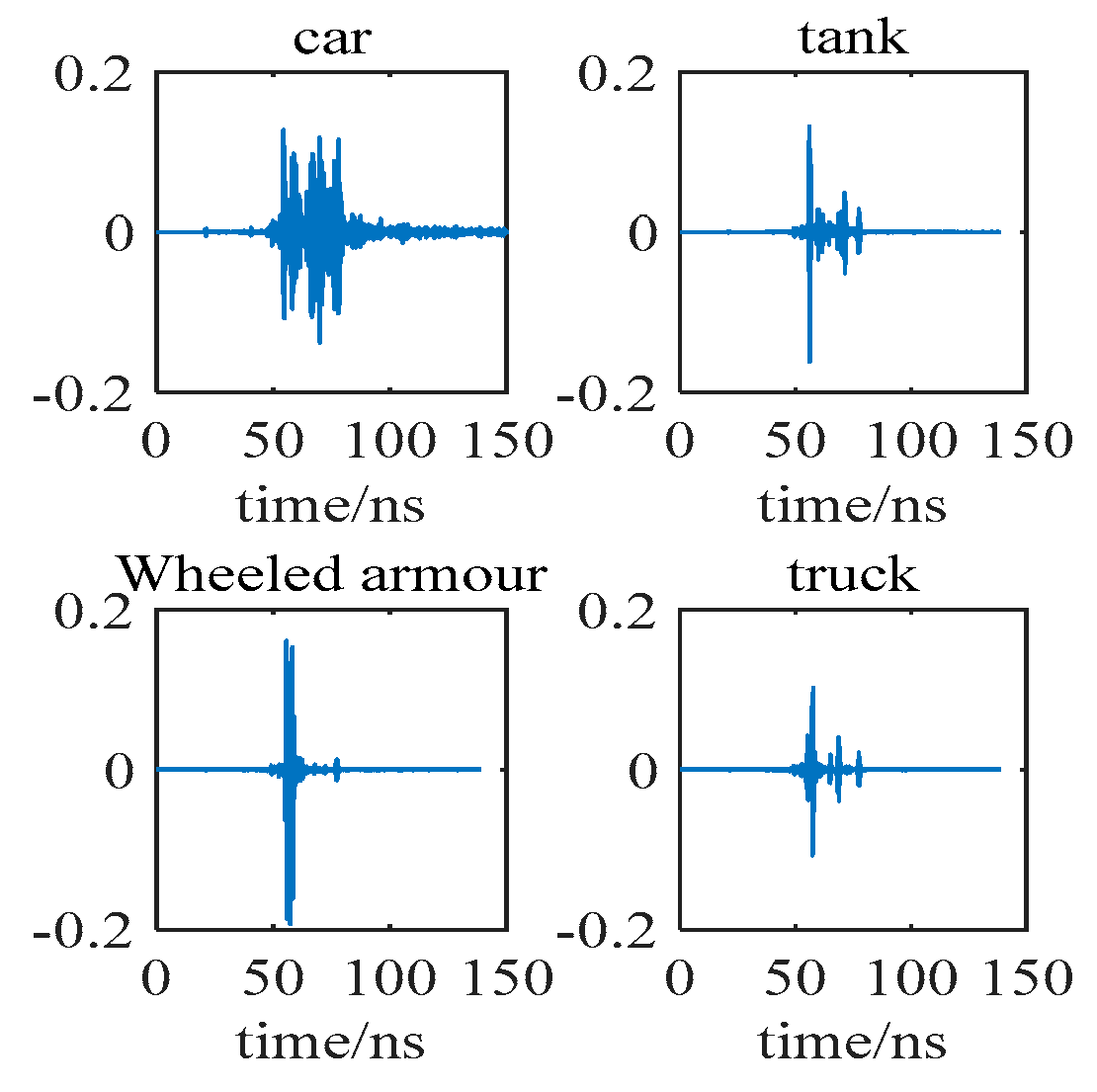
The model is used to form a jungle space unit of 10 m × 11 m × 6 m, which is fully capable of masking the hidden targets in the jungle, as shown in Figure 2. We place four kinds of target vehicles under the jungle as follows: a wheeled armored vehicle, a tracked vehicle, a van truck, and a sedan. The four kinds of vehicles are modeled in 3ds Max. The primary material of the vehicles is steel, and the sizes of the vehicles are shown in Table 2. The sensor is placed at a distance of 10 m from the target. The transmitting signal of the carrier-free ultra-wideband sensor is set as a Gaussian pulse with a center frequency of 3 GHz. Figure 3 shows the transmitting signal time-domain waveform and frequency-domain waveform. The transmitting and receiving antenna is a Vivaldi antenna, as shown in Figure 4. The size of the antenna is 57 mm × 50 mm, and it operates in the frequency band of 0.89–5.02 GHz with almost omnidirectional radiation from the H-plane. The simulation is performed with a single transmitter and single receiver sensor. The pitch angle of the sensor is set to 30°, while the azimuth angle is set to vary from 0 to 360° at 2° intervals to obtain four vehicle echoes. When the sensor azimuth is at 0°, the four vehicle echoes are as shown in Figure 5.
2.3. Markov Transfer Field
Markov Transfer Field (MTF) is a time series image coding method based on the Markov transfer matrix.
For the conversion of 1D time series into MTF images, the time signal is divided into Q quantile bins. We label the discrete quantile bins with a quantile (). According to the division of quantile bins, each time domain amplitude is mapped to the corresponding quantile bin. The Markov transfer matrix W is constructed by calculating the leap between quartiles along the time axis as a first-order Markov chain and is expressed as follows:
where is the probability that quartile is followed by quartile , . Typically, is considered to be the frequency with which quartile is transferred to quartile .
The time factor is usually considered, and the matrix M is constructed to capture the dependency between the location and the time step. The matrix M extends the matrix W by arranging each probability along the time order according to the relationship between the quartiles and the time step, retaining the additional time information. The expression of the matrix M is as follows:
The time-domain echo signal is converted into a two-dimensional image through the Markov transfer field, as shown in Figure 6.
3. The Improved RepVGG Network
In this section, we describe the self-attention module, the structural details of the improved RepVGG network, and the composite sparsemax loss function and provide the overall network structure and specific hyperparameters.
3.1. Self-Attention Module
The literature indicates that combining convolution and self-attention can improve the performance of network image classification [36]. To better extract the features of the image, improve the classification accuracy of the network, and enhance the generalization ability of the network, RepVGG is improved by embedding the self-attention module to make the network perform better.
Three convolution layers (query convolution, key convolution, and value convolution) are used to compute the query, key, and value vectors, respectively. The query and key vectors are used to compute the attentional weights, and the value vector represents the information that the network needs to retain. Specifically, the input tensor x can be expanded into the shape of batch size, channels, height, and width. We perform a convolution operation on it with the query convolution layer and key convolution layer to obtain the query and key vectors, compute the matrix multiplication between query and key, and then normalize the energy with a softmax function to obtain the attention weights, and, finally, convolve the input with value convolution layer to obtain the value vector. Considering that the attention weights already have the importance of each element in the input tensor, we multiply the value vector and attention weights to obtain the significant segments of the input. Finally, the output of this self-attention module is the input tensor plus the output of the self-attention mechanism. In addition, before summation, we multiply them by the trainable scaling parameter gamma and the trainable scaling parameter beta, respectively. The network’s perception of image features is enhanced by incorporating the self-attention module, and we control the degree of enhancement through the gamma parameter and the beta parameter. Figure 7 illustrates the structure of the self-attention module.
We add the self-attention module at the output of stage 0 to improve the network’s ability to extract features of the image and better capture the complex relationships among features. The self-attention module is added before the linear layer classification output at stage 4 to improve the classification accuracy of the network.
3.2. Framework and Parameters of the RepVGG
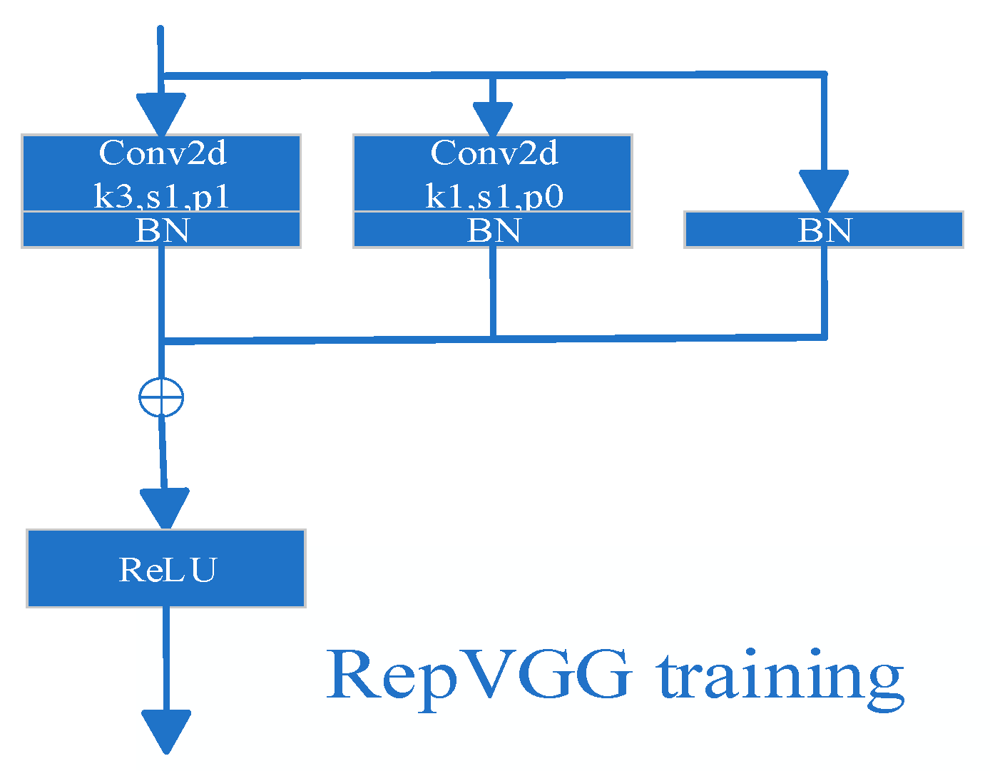
In this section, we explain the structural details of the RepVGG network and give the structure of the overall network and specific hyperparameters. The RepVGG network has different structures in the training stage and inference stage. In the training stage, the network has a multi-branch topology, as shown in Figure 8. In the inference stage, the network structure is similar to the architecture of VGG. The inference structure consists of a stack of 3 × 3 convolutions and ReLU functions. This decoupling of the training and inference architectures is achieved by a reparameterization technique of the structure. Hence, the network is called RepVGG.
In the training stage, a multi-branch network structure is used, as shown in Figure 9, using identity and 1 × 1 branches to construct the residual block for the training stage. The formula is as follows:
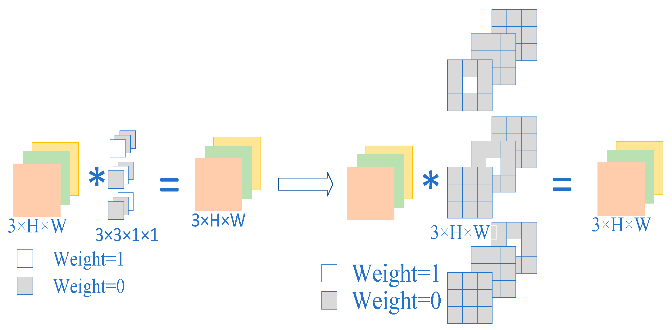
In the inference stage, as shown in Figure 10 and Figure 11, the structure reparameterization process is divided into the following three steps: Step 1. Fuse the 2D Convolution layer with the BN (batch normalization) layer. Step 2. Convert the branches that have only the BN layer into a single 2D convolution layer. Step 3. Fuse the convolution layers in each branch into one convolution layer.
In the first step, the 2D convolution layer and BN layers are fused. For the convolution layer, the number of channels in each convolution kernel is the same as the number of channels in the input feature map. The number of convolution kernels determines the number of channels in the output feature map.
The BN layer (the inference stage) contains the following four main parameters: mean , variance , learning scaling factor , and bias , where the mean and variance are statistically obtained during training. The learning scaling factor and the bias are learned during training. The output of the convolution layer is:
The output of the BN layer is:
Then, bring the output of the convolution layer into the BN layer:
Simplify:
We can obtain the fusion layer through Formula (11).
In the second step, the identity branch, the branch with the only BN layer, is converted into a 2D convolution layer. A 3 × 3 convolution layer is built, which performs identity mapping, i.e., the input feature map and output feature map are constant. Following the first step, the convolution layer is fused with the BN layer.
In the third step, three branches are converted into a single convolution kernel, where the 1 × 1 convolutional kernel is converted into the 3 × 3 convolution kernel by zero padding. The formula is as follows:
where means the convolution operation.
Finally, the overall structure of the improved RepVGG is shown in Figure 12. The different target echoes are converted into two-dimensional images by the Markov Transfer Field. During training, the images pass through the self-attention module, which helps the network better capture the formation of the RepVGG block in stage 0. The images then pass through the four RepVGG blocks and the 2D adaptive average pooling layer and are sent to the self-attention module again, which improves the performance of feature classification and the generalization ability of the network. Then, they are sent to the linear for classification after flattening. The network structural parameters of the improved RepVGG are shown in Table 3.
3.3. Improved Loss Function
The traditional cross-entropy loss function has the advantages of fast convergence, good generalization robustness, high classification accuracy, etc., but it is not perfect. The sparsity of the cross-entropy loss function is poor for the category imbalance. The cross-entropy loss function will pay more attention to the category with more samples and is not sensitive enough to the category with fewer samples. In the case of a small sample size, the network in the training process is prone to overfitting. The cross-entropy loss function focuses more on the prediction result of classification rather than the boundary. Therefore, we propose a new sparsity loss function, SparsityLoss. The method is designed not only to consider the prediction accuracy of the model, but also to incorporate a penalty on the model complexity to promote the sparsity of the model, which can reduce the risk of overfitting, deal with unbalanced classification problems, and better handle noisy data, thus improving the generalization ability and robustness of the model.
SparsityLoss is a hybrid loss function that combines L1 regularization and cross-entropy loss. SparsityLoss was originally designed to incorporate a model complexity penalty to steer the model in the direction of greater simplicity and sparsity while ensuring model learning efficiency and prediction accuracy. This improves the generalization ability of the model. The core component of SparsityLoss consists of the following three parts: the loss of the squared difference between the output of Softmax and the target value, the loss of cross-entropy, and the L1 regularization term. The loss of the squared difference between the output of Softmax and the target value strengthens the match between the target class probability distribution and the predicted probability distribution. The L1 regularization term imposes sparsity constraints on the model. Cross entropy loss is used to deal with multiclassification problems.
The procedure of the loss function is described in Algorithm 1. SparsityLoss optimization balances the predictive accuracy and complexity of the model by adjusting the weights of the components in the loss function. Firstly, we operate on the model output (Softmax). A fixed value (1/N) is subtracted from the output of each sample. N is the recognition category. Its difference from the target label is measured by squared difference loss. In addition, we introduce an L1 regularization term that directly penalizes the absolute value of the model weights. It drives the weights to converge to zero, thus increasing the sparsity of the model. Finally, we deal with the classification problem through cross-entropy loss to effectively improve the classification accuracy of the model.
| Algorithm 1 RepVGG with a Modified Loss Function. |
| Step 1: Calculate the softmax value of the model classification outputs. |
| Step 2: Calculate the output of sparsity. where is the number of categories. |
| Step 3: Weighted summation. |
We trained the model by combining cross-entropy and squared error. This helps to reduce the effect of extreme predictive values and steadily reduce the loss during training. This combination strategy typically increases the model’s generalization ability and tolerance to noise. The L1 loss adds a constraint on the sparsity of the weights. This design facilitates the model to learn a sparser distribution of weights, which can reduce the complexity of the model, improve its interpretability, and help prevent the occurrence of the overfitting phenomenon. The SparsityLoss function proposed in this paper provides a new optimization scheme for deep learning model training. By introducing a penalty for model complexity in the loss function, SparsityLoss effectively promotes model sparsity and improves the generalization ability of the model.
4. Experiment and Results
In this section, the improved RepVGG is simulated and compared with several classical network models. Experimental details are given, and the results are analyzed.
4.1. Dataset Description and Experimental Details
We simulated four types of vehicle echoes from the sensor in the jungle environment, with the sensor 10 m away from the center of the vehicle, in the direction of 30° pitch angle, and collect echoes at 2° intervals in azimuth. The ratio of the training set, validation set, and test set is 3:1:1, the SNR of the training set is varied from 0 to 25 at 5 dB intervals, the batch size is set to 20, the learning rate is set to 5 × 10⁻⁴, and the epochs are 100. The SNR is defined by the following equation:
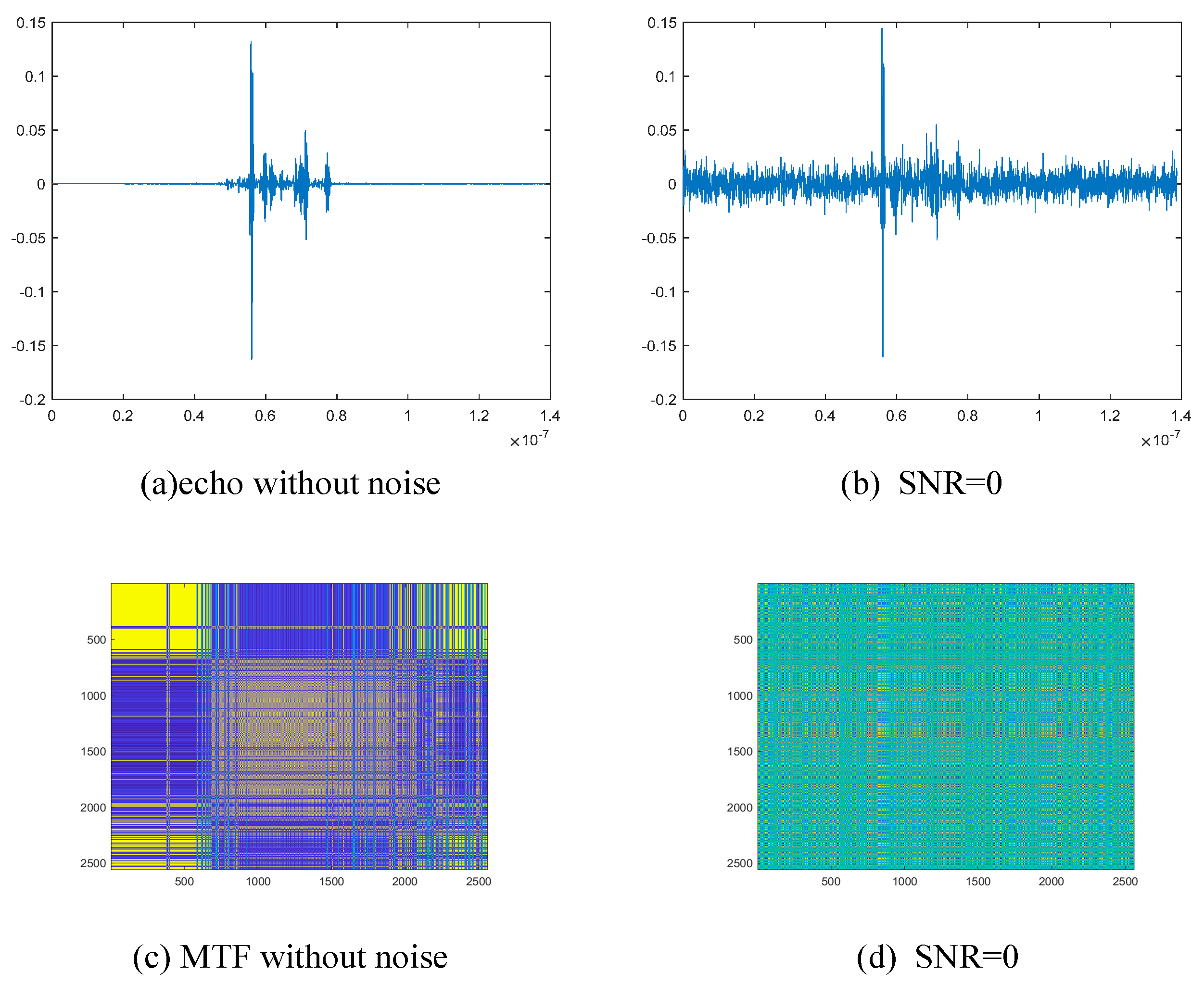
where is the power of the signal, is the noise power, is the signal amplitude, and is the noise amplitude. As the SNR increases, the lower the noise power and the higher the signal power, the cleaner the signal is. We add Gaussian noise with different SNR ratios to the echo, where the SNR is 0 dB, 5 dB, 10 dB, 15 dB, 20 dB, and 25 dB, as shown in Figure 13. In order to assess the efficiency of the model classification, common measures in machine learning, including the confusion matrix, overall classification accuracy (OA), and the kappa coefficient (Ka), are utilized.
4.2. Performance Analysis of the Improved RepVGG
In a real scenario, a sensor does not just receive the target electromagnetic scattering echoes, but it also other types of noise. To test the noise robustness of the improved RepVGG that we propose, we simulated its recognition performance under different SNRs. Meanwhile, to better analyze the recognition performance of the network, we introduced the confusion matrix and the kappa coefficient.
The recognition performance of the improved RepVGG under different SNRs is revealed in Figure 14 and Figure 15. At SNR = 0 dB, the OA of the MTF of the four vehicle targets is the lowest, which still achieves a recognition rate of 91%. Starting from the SNR of 0 dB, every 10 dB increase in SNR results in improved recognition performance. The recognition rate of the network reaches 93.8% when the SNR = 25 dB. The recognition rate of the network reaches the highest when there is no noise, which reaches 95.1%. It is observed that the recognition rates remain constant when the SNR is 10 dB compared with 15 dB, as well as when the SNR is 20 dB compared with 25 dB. Furthermore, starting from the SNR of 0 dB, there is an overall upward trend in recognition performance. Figure 15 reveals that the kappa coefficient of the network recognition also becomes larger and slowly higher, with a kappa coefficient of 0.88 when SNR = 0 dB. When SNR = 25 dB, the kappa coefficient is 0.9167. The kappa coefficient of the network reaches 0.9352 when we do not add noise to the echo. An evaluation with a kappa coefficient greater than 0.8 implies that the classifier has very good performance. An evaluation of a network with a kappa coefficient greater than 0.8 means that the classifier performs very well in the task being evaluated. The network has high accuracy and consistency and can be trusted to classify the samples correctly. The kappa coefficients of the network are all greater than 0.8 in the case when the SNR is greater than 0 dB. Therefore, the improved RepVGG has high accuracy and consistency.
The confusion matrix for the recognition results of the network is depicted in Figure 17 at various SNRs of 0 dB, 5 dB, 10 dB, 15 dB, 20 dB, and 25 dB and in Figure 16 without noise. As shown in the figure, the recognition rate of both cars and wheeled armored vehicles reaches 100% during the recognition process for different SNRs and noiseless MTF maps, indicating that cars and wheeled armored vehicles are highly discriminated by the feature vectors extracted by the network. At SNR = 0 dB, the network recognized 10 samples of trucks as tracked vehicles, while 3 samples of tracked vehicles were recognized as trucks. At SNR = 5 dB, the network recognized five samples of trucks as tracked vehicles and eight samples of tracked vehicles as trucks. At SNR = 10 dB, the network recognized two samples of trucks as tracked vehicles and nine samples of tracked vehicles as trucks. At SNR = 15 dB, the network recognized six samples of trucks as tracked vehicles and five samples of tracked vehicles as trucks. At SNR = 20 dB, the network recognized one sample of trucks as tracked vehicles and eight samples of tracked vehicles as trucks. At SNR = 25 dB, the network recognized three samples of trucks as tracked vehicles and six samples of tracked vehicles as trucks. In the noise-free condition, the network identified four samples of tanks as trucks and three samples of trucks as tanks. In the case of a low SNR, because the electromagnetic scattering characteristics of tracked vehicles and truck vehicles are more similar under some observation angles, the number of scattering points and the distribution in the echo are closer, the MTF images generated by the echo lead to a low differentiation of the distribution of the feature vectors extracted by the network, and with the increase in the SNR, there is a significant improvement in the network’s ability to distinguish between the two vehicles. The overall recognition rate of the network is greater than 90%, with the SNR not less than 0 dB. The experimental results show that the network has good recognition accuracy and noise robustness.
4.3. Network Performance Comparison
4.3.1. Recognition Performance Comparison
We proposed an improved RepVGG network and validated its recognition performance by comparing and analyzing it alongside other classical network recognition methods. These methods include DenseNet, Inception, VGG, ResNet, and LeNet. We plotted the recognition performance curves under different SNRs, as shown in Table 4 and Table 5. As can be seen in Table 4, under a low SNR, the improved RepVGG network has a significant improvement in recognition accuracy compared with the traditional classical neural network models. Among the compared network models, the VGG has the highest recognition rate of 87.5%, ResNet has the lowest recognition rate of 79.8%, and the improved RepVGG network reaches 90.97% at SNR = 0 dB, which is 3% higher than VGG and 10% higher than ResNet. When the SNR gradually increases, the recognition accuracy of each model is significantly improved. At SNR = 25 dB, the recognition accuracy of each model exceeds 88%, the recognition rate of VGG is the highest at 93%, and Inception is the lowest at 88.5%. The improved RepVGG network reaches 93.8%, which is 0.8% higher than VGG and 4.9% higher than Inception.
Table 5 shows the variation in the kappa coefficient at different SNRs. At a low SNR, the improved RepVGG network’s kappa coefficient reaches 0.88, while among the compared network models, VGG has the highest kappa coefficient of 0.833, and ResNet has the lowest kappa coefficient of 0.731. When the SNR gradually increases, the kappa coefficient of each model improves significantly. At SNR = 25 dB, each model exceeds 0.87. The kappa coefficient of the improved RepVGG network is 0.9167. Among the compared network models, VGG has the highest kappa coefficient of 0.907, and Inception has the lowest kappa coefficient of 0.852. With the gradual increase in the SNR, the kappa coefficient of the improved RepVGG network is always the highest, and compared with the other networks, the improved RepVGG network has the best consistency. In the comprehensive analysis, the improved RepVGG network has higher classification accuracy, better noise robustness, and sound recognition performance.
4.3.2. Ablation Experiment
To demonstrate the advantage that the self-attention module and sparse loss function bring to the recognition process, we conducted some ablation experiments, as shown in Figure 18. When the classical RepVGG network was added to the self-attention module alone, the recognition rate of the network increased from 93.1% to 94.4%. When the sparse loss function alone was added to the classical RepVGG network, the recognition rate of the network increased from 93.1% to 93.8%. When both the self-attention module and the sparse loss function were also added to the VGG network, the recognition rate of the model increased from 93.08% to 93.75%. This is a good indication that the self-attention module and the sparsity loss function are more helpful in improving the recognition accuracy of the network.
5. Conclusions
In this work, we converted the traditional one-dimensional sensor echo into a two-dimensional image by MTF transformation to better capture the time-series relationship of the signal. The improved RepVGG network is proposed for the identification of carrier-free ultra-wideband sensor jungle targets. In different stages, we introduce the self-attention module to improve the ability to extract the features of target echoes and enhance robustness. Meanwhile, the composite sparse loss function is put forward to improve the classification accuracy. The experimental results show that the improved RepVGG network improves the recognition performance and noise immunity, and the OA and kappa coefficients of the proposed method are better than the five methods proposed in the literature. In our future work, we will carry out research on the carrier-free ultra-wideband sensor for water targets and airspace targets for better application in practical road driving, field exploration, and other fields.
Author Contributions
Writing—original draft, J.L.; Supervision, S.Z.; Funding acquisition, L.Z.; Formal analysis, S.C.; Investigation, L.H.; Methodology, X.L.; Software, K.C. All authors have read and agreed to the published version of the manuscript.
Funding
This work was supported in part by the National Natural Science Foundation of China (NSFC) under Grant 62301260, and Grant 62271261, the Natural Science Foundation of Jiangsu Province under Grant BK20220941, the Fundamental Research Funds for the Central Universities under Grant 30922010717.
Data Availability Statement
The datasets presented in this article are not readily available because the data are part of an on-going study.
Conflicts of Interest
The authors declare no conflict of interest.
References
- Li, X.; Xiao, Z.; Zhu, Y.; Zhang, S.; Chen, S. Carrier-Free UWB Sensor Small-Sample Terrain Recognition Based on Improved ACGAN With Self-Attention. IEEE Sens. J. 2022, 22, 8050–8058. [Google Scholar] [CrossRef]
- Shen, Y.; Chen, X.; Rhee, W.; Wang, Z. A second-order multi-bit ΔΣ TDC for high resolution IR-UWB radar systems. In Proceedings of the 2014 IEEE International Wireless Symposium (IWS 2014), Xi’an, China, 24–26 March 2014; pp. 1–4. [Google Scholar]
- Tsang, T.K.K.; El-Gamal, M.N. Ultra-wideband (UWB) communications systems: An overview. In Proceedings of the 3rd International IEEE-NEWCAS Conference, Quebec, QC, Canada, 19–22 June 2005; pp. 381–386. [Google Scholar]
- Naveena, M.; Singh, D.K.; Singh, H. Design of UHF band UWB antenna for foliage penetration application. In Proceedings of the 2017 IEEE International Conference on Antenna Innovations & Modern Technologies for Ground, Aircraft and Satellite Applications (iAIM), Bangalore, India, 24–26 November 2017; pp. 1–3. [Google Scholar]
- Kim, S.Y.; Han, H.G.; Kim, J.W.; Lee, S.; Kim, T.W. A Hand Gesture Recognition Sensor Using Reflected Impulses. IEEE Sens. J. 2017, 17, 2975–2976. [Google Scholar] [CrossRef]
- Ye, S.; Chen, J.; Liu, L.; Zhang, C.; Fang, G. A novel compact UWB ground penetrating radar system. In Proceedings of the 2012 14th International Conference on Ground Penetrating Radar (GPR), Shanghai, China, 4–8 June 2012; pp. 71–75. [Google Scholar]
- Anabuki, M.; Okumura, S.; Sakamoto, T.; Saho, K.; Sato, T.; Yoshioka, M.; Inoue, K.; Fukuda, T.; Sakai, H. High-resolution imaging and separation of multiple pedestrians using UWB Doppler radar interferometry with adaptive beamforming technique. In Proceedings of the 2017 11th European Conference on Antennas and Propagation (EUCAP), Paris, France, 19–24 March 2017; pp. 469–473. [Google Scholar]
- Numan, P.E.; Park, H.; Lee, J.; Kim, S. Machine Learning-Based Joint Vital Signs and Occupancy Detection With IR-UWB Sensor. IEEE Sens. J. 2023, 23, 7475–7482. [Google Scholar] [CrossRef]
- Ni, Y.; Chen, H. Detection of underwater carrier-free pulse based on time-frequency analysis. J. Netw. 2013, 8, 205. [Google Scholar] [CrossRef]
- Li, C.; Yang, S.-T.; Ling, H. ISAR imaging of a windmill—Measurement and simulation. In Proceedings of the 8th European Conference on Antennas and Propagation (EuCAP 2014), The Hague, The Netherlands, 6–11 April 2014; pp. 1–5. [Google Scholar]
- Bai, Z.; Zhang, W.; Xu, S.; Liu, W.; Kwak, K. On the performance of multiple access DS-BPAM UWB system in data and image transmission. In Proceedings of the IEEE International Symposium on Communications and Information Technology, ISCIT 2005, Beijing, China, 12–14 October 2005; pp. 851–854. [Google Scholar]
- Zhang, S.; Pan, X.; Mu, H. A multi-pedestrian cooperative navigation and positioning method based on UWB technology. In Proceedings of the 2020 IEEE International Conference on Artificial Intelligence and Information Systems (ICAIIS), Dalian, China, 20–22 March 2020; pp. 260–264. [Google Scholar]
- Wang, X.; Zhang, S.; Chen, S.; Hou, L.; Zhu, L. An Antijamming Method Based on Multichannel Singular Spectrum Analysis and Affinity Propagation for UWB Ranging Sensors. IEEE Sens. J. 2023, 23, 11869–11878. [Google Scholar] [CrossRef]
- Xia, Z.; Wang, P.; Dong, G.; Liu, H. Radar HRRP Open Set Recognition Based on Extreme Value Distribution. IEEE Trans. Geosci. Remote Sens. 2023, 61, 5102416. [Google Scholar] [CrossRef]
- Li, X.; Ouyang, W.; Pan, M.; Lv, S.; Ma, Q. Continuous Learning Method of Radar HRRP Based on CVAE-GAN. IEEE Trans. Geosci. Remote Sens. 2023, 61, 5107819. [Google Scholar] [CrossRef]
- Zhang, Y.; Kong, Y. Target Recognition of HRRP Based on CNN with Multi-Axis Attention and Residual Connections. In Proceedings of the 2022 IEEE 24th Int Conf on High Performance Computing & Communications; 8th Int Conf on Data Science & Systems; 20th Int Conf on Smart City; 8th Int Conf on Dependability in Sensor, Cloud & Big Data Systems & Application (HPCC/DSS/SmartCity/DependSys), Hainan, China, 18–20 December 2022; pp. 2338–2344. [Google Scholar]
- Zhang, Y.-P.; Zhang, L.; Kang, L.; Wang, H.; Luo, Y.; Zhang, Q. Space Target Classification with Corrupted HRRP Sequences Based on Temporal–Spatial Feature Aggregation Network. IEEE Trans. Geosci. Remote Sens. 2023, 61, 5100618. [Google Scholar] [CrossRef]
- Kong, Y.; Feng, D.; Zhang, J. Radar HRRP Target Recognition Based on Composite Deep Networks. In Proceedings of the 2022 International Applied Computational Electromagnetics Society Symposium (ACES-China), Xuzhou, China, 28–31 July 2022; pp. 1–5. [Google Scholar]
- Wang, X.; Wang, P.; Song, Y.; Li, J. Recognition of HRRP sequence based on TCN with attention and elastic net regularization. In Proceedings of the 2022 International Conference on Image Processing, Computer Vision and Machine Learning (ICICML), Xi’an, China, 28–30 October 2022; pp. 346–351. [Google Scholar]
- Zhu, Y.; Zhang, S.; Li, X.; Zhao, H.; Zhu, L.; Chen, S. Ground Target Recognition Using Carrier-Free UWB Radar Sensor with a Semi-Supervised Stacked Convolutional Denoising Autoencoder. IEEE Sens. J. 2021, 21, 20685–20693. [Google Scholar] [CrossRef]
- Zhu, L.; Sun, Y.; Zhang, S. Multi-Angle Recognition of Vehicles Based on Carrier-Free UWB Sensor and Deep Residual Shrinkage Learning. IEEE Microw. Wirel. Compon. Lett. 2022, 32, 927–930. [Google Scholar] [CrossRef]
- Zhu, Y.; Chen, S.; Li, X.; Zhang, S.; Zhu, L. Multi-Task Self-Supervised Learning for Vehicle Classification Based on Carrier-Free UWB Radars. IEEE Trans. Instrum. Meas. 2022, 71, 2515312. [Google Scholar] [CrossRef]
- Lyu, C.; Huo, Z.; Cheng, X.; Jiang, J. Alimasi and H. Liu. Distributed Optical Fiber Sensing Intrusion Pattern Recognition Based on GAF and CNN. J. Light. Technol. 2020, 38, 4174–4182. [Google Scholar] [CrossRef]
- Tian, M.; Li, Q.; Xv, C.; Yang, Y.; Li, Z. Coal-rock Interface Recognition Method Based on GAF-deep Learning. In Proceedings of the 2021 IEEE 5th Conference on Energy Internet and Energy System Integration (EI2), Taiyuan, China, 22–24 October 2021; pp. 4029–4033. [Google Scholar]
- Wu, J.; Zhong, Y.; Chen, A. Radio Modulation Classification Using STFT Spectrogram and CNN. In Proceedings of the 2021 7th International Conference on Computer and Communications (ICCC), Chengdu, China, 10–13 December 2021; pp. 178–182. [Google Scholar]
- Ong, K.L.; Lee, C.P.; Lim, H.S.; Lim, K.M.; Alqahtani, A. Mel-MViTv2: Enhanced Speech Emotion Recognition with Mel Spectrogram and Improved Multiscale Vision Transformers. IEEE Access 2023, 11, 108571–108579. [Google Scholar] [CrossRef]
- Vaswani, A.; Shazeer, N.; Parmar, N.; Uszkoreit, J.; Jones, L.; Gomez, A.N.; Kaiser, Ł.; Polosukhin, I. Attention is all you need. Adv. Neural Inf. Process. Syst. 2017, 30. [Google Scholar]
- Bello, I.; Zoph, B.; Vaswani, A.; Shlens, J.; Le, Q.V. Attention augmented convolutional networks. In Proceedings of the IEEE/CVF International Conference on Computer Vision, Seoul, Republic of Korea, 27 October–2 November 2019; pp. 3286–3295. [Google Scholar]
- Sun, L.; Zou, H.; Wei, J.; Li, M.; Cao, X.; He, S.; Liu, S. Semantic Segmentation of High-Resolution Remote Sensing Images Based on Sparse Self-Attention. In Proceedings of the IGARSS 2022—2022 IEEE International Geoscience and Remote Sensing Symposium, Kuala Lumpur, Malaysia, 17–22 July 2022; pp. 3492–3495. [Google Scholar]
- Chowdhury, T.; Rahnemoonfar, M. Self Attention Based Semantic Segmentation on a Natural Disaster Dataset. In Proceedings of the 2021 IEEE International Conference on Image Processing (ICIP), Anchorage, AK, USA, 19–22 September 2021; pp. 2798–2802. [Google Scholar]
- Chen, Q.; Dai, X.; Song, X.; Liu, G. ITSC Fault Diagnosis for Five Phase Permanent Magnet Motors by Attention Mechanisms and Multiscale Convolutional Residual Network. IEEE Trans. Ind. Electron. 2024, 71, 9737–9746. [Google Scholar] [CrossRef]
- Wang, J.; Guo, J.; Xu, Z. Cross-view Gait Recognition Model Combining Multi-Scale Feature Residual Structure and Self-attention Mechanism. IEEE Access 2023, 11, 127769–127782. [Google Scholar] [CrossRef]
- Fu, X.; Liu, J.; Yu, P. Multi-scale Convolutional Neural Networks Based on Self-attention And Residual Network for Industrial Equipment Fault Diagnosis. In Proceedings of the 2023 CAA Symposium on Fault Detection, Supervision and Safety for Technical Processes (SAFEPROCESS), Yibin, China, 22–24 September 2023; pp. 1–6. [Google Scholar]
- Wang, G.; Tang, L.; Yang, Z.; Yan, L.; Liu, P.; Qu, H. Deep CNN-RNN with Self-Attention Model for Electric IoT Traffic Classification. In Proceedings of the 2023 4th International Conference on Big Data & Artificial Intelligence & Software Engineering (ICBASE), Nanjing, China, 25–27 August 2023; pp. 363–368. [Google Scholar]
- Ding, X.; Zhang, X.; Ma, N.; Han, J.; Ding, G.; Sun, J. RepVGG: Making VGG-style ConvNets Great Again. In Proceedings of the 2021 IEEE/CVF Conference on Computer Vision and Pattern Recognition (CVPR), Nashville, TN, USA, 20–25 June 2021; pp. 13728–13737. [Google Scholar]
- Cordonnier, J.B.; Loukas, A.; Jaggi, M. On the relationship between self-attention and convolutional layers. arXiv 2019, arXiv:1911.03584. [Google Scholar]
Figure 1.
Individual tree model. (a) Branches and trunk. (b) Overall tree model.

Figure 2.
Different perspectives of targets. (a) Side and top view of a wheeled armored vehicle. (b) Side and top view of a tracked vehicle. (c) Side and top view of a van truck. (d) Side and top view of a sedan.
Figure 2.
Different perspectives of targets. (a) Side and top view of a wheeled armored vehicle. (b) Side and top view of a tracked vehicle. (c) Side and top view of a van truck. (d) Side and top view of a sedan.


Figure 3.
Gaussian pulse.

Figure 4.
Vivaldi antenna. (a) Antenna structure; (b) 3 GHz antenna far-field directional view.

Figure 5.
Echoes of four kinds of vehicles.

Figure 6.
Time domain echo and MTF image. (a) The time-domain echo. (b) MTF image.

Figure 7.
The structure of the self-attention module.

Figure 8.
The structure of the RepVGG.

Figure 9.
Training stage.

Figure 10.
Diagram of fusion.

Figure 11.
The workflows of fusion.

Figure 12.
The overall structure of the improved RepVGG.

Figure 13.
Time domain echo and MTF images without noise and at SNR = 0.

Figure 14.
OA at a different SNR.

Figure 15.
Kappa coefficients at a different SNR.

Figure 16.
Confusion matrix without noise.

Figure 17.
The confusion matrixes at SNR = 0 dB, 5 dB, 10 dB, 15 dB, 20 dB, and 25 dB. (a) SNR = 0 dB, (b) SNR = 5 dB, (c) SNR = 10 dB, (d) SNR = 15 dB, (e) SNR = 20 dB, and (f) SNR = 25 dB.
Figure 17.
The confusion matrixes at SNR = 0 dB, 5 dB, 10 dB, 15 dB, 20 dB, and 25 dB. (a) SNR = 0 dB, (b) SNR = 5 dB, (c) SNR = 10 dB, (d) SNR = 15 dB, (e) SNR = 20 dB, and (f) SNR = 25 dB.


Figure 18.
Comparison of the ablation experiment.


Table 1.
The layers of the model and the composition of the layers.
| Model Layers | Layer Composition |
|---|---|
| Canopy layer | Scatterers of leaves, stems, and branches |
| Trunk layer | Scatterers of trunks perpendicular to the ground |
| Ground layer | Soil surface with corresponding dielectric constant |
Table 2.
The sizes of the vehicles.
| Vehicle Type | Vehicle Size |
|---|---|
| wheeled armored vehicle | 4 m × 2 m × 2 m |
| tracked vehicle | 7 m × 2.2 m × 2.2 m |
| van truck | 8.5 m × 2.5 m × 2.7 m |
| sedan | 4.58 m × 1.77 m × 1.42 m |
Table 3.
The network structure parameters of the improved RepVGG.
| Stage/Type | The Number of RepVGG Blocks | The Number of Self-Attention Modules | Input Size | Input Channels | Output Size | Output Channels | Stride |
|---|---|---|---|---|---|---|---|
| Stage 0 | 1 | 1 | 256 × 256 | 3 | 128 × 128 | 64 | 2 |
| Stage 1 | 1 | 0 | 128 × 128 | 64 | 64 × 64 | 320 | 2 |
| Stage 2 | 1 | 0 | 64 × 64 | 320 | 32 × 32 | 512 | 2 |
| Stage 3 | 1 | 0 | 32 × 32 | 512 | 16 × 16 | 768 | 2 |
| Stage 4 | 1 | 0 | 16 × 16 | 768 | 8 × 8 | 1280 | 2 |
| Self-attention | - | 1 | 8 × 8 | 1280 | 8 × 8 | 1280 | 1 |
| AdaptiveAvgPool2d | - | - | 8 × 8 | 1280 | 1 × 1 | 1280 | - |
| Linear | - | - | 1 × 1 | 1280 | 1 | 4 | - |
Table 4.
OA of the six methods with SNR.
| OA | The Improved RepVGG | DenseNet | Inception | LeNet | ResNet | VGG |
|---|---|---|---|---|---|---|
| SNR = 0 | 90.97% | 79.86% | 85.42% | 86.81% | 79.86% | 87.50% |
| SNR = 5 | 91.10% | 83.33% | 85.42% | 86.81% | 80.56% | 88.89% |
| SNR = 10 | 92.40% | 85.42% | 85.42% | 90.28% | 86.81% | 88.89% |
| SNR = 15 | 92.40% | 87.5% | 86.11% | 91.67% | 86.11% | 88.89% |
| SNR = 20 | 93.80% | 87.5% | 86.11% | 92.36% | 88.89% | 90.97% |
| SNR = 25 | 93.80% | 90.97% | 88.89% | 92.36% | 90.28% | 93.06% |
| Noise-free | 95.14% | 91.18% | 92.36% | 94.44% | 90.48% | 93.06% |
Table 5.
KAPPA coefficient the six methods with SNR.
| Kappa Coefficient | The Improved RepVGG | DenseNet | Inception | LeNet | ResNet | VGG |
|---|---|---|---|---|---|---|
| SNR = 0 | 0.8796 | 0.731 | 0.806 | 0.824 | 0.731 | 0.833 |
| SNR = 5 | 0.8796 | 0.778 | 0.806 | 0.824 | 0.741 | 0.852 |
| SNR = 10 | 0.8981 | 0.806 | 0.806 | 0.87 | 0.824 | 0.852 |
| SNR = 15 | 0.8981 | 0.833 | 0.815 | 0.889 | 0.815 | 0.843 |
| SNR = 20 | 0.9167 | 0.833 | 0.815 | 0.889 | 0.852 | 0.88 |
| SNR = 25 | 0.9167 | 0.88 | 0.852 | 0.889 | 0.87 | 0.907 |
| Noise-free | 0.9352 | 0.882 | 0.898 | 0.926 | 0.873 | 0.907 |
Disclaimer/Publisher’s Note: The statements, opinions and data contained in all publications are solely those of the individual author(s) and contributor(s) and not of MDPI and/or the editor(s). MDPI and/or the editor(s) disclaim responsibility for any injury to people or property resulting from any ideas, methods, instructions or products referred to in the content. |
© 2024 by the authors. Licensee MDPI, Basel, Switzerland. This article is an open access article distributed under the terms and conditions of the Creative Commons Attribution (CC BY) license (https://creativecommons.org/licenses/by/4.0/).
Share and Cite
MDPI and ACS Style
Li, J.; Zhang, S.; Zhu, L.; Chen, S.; Hou, L.; Li, X.; Chen, K. Carrier-Free Ultra-Wideband Sensor Target Recognition in the Jungle Environment. Remote Sens. 2024, 16, 1549. https://0-doi-org.brum.beds.ac.uk/10.3390/rs16091549
AMA Style
Li J, Zhang S, Zhu L, Chen S, Hou L, Li X, Chen K. Carrier-Free Ultra-Wideband Sensor Target Recognition in the Jungle Environment. Remote Sensing. 2024; 16(9):1549. https://0-doi-org.brum.beds.ac.uk/10.3390/rs16091549
Chicago/Turabian StyleLi, Jianchao, Shuning Zhang, Lingzhi Zhu, Si Chen, Linsheng Hou, Xiaoxiong Li, and Kuiyu Chen. 2024. "Carrier-Free Ultra-Wideband Sensor Target Recognition in the Jungle Environment" Remote Sensing 16, no. 9: 1549. https://0-doi-org.brum.beds.ac.uk/10.3390/rs16091549
Note that from the first issue of 2016, this journal uses article numbers instead of page numbers. See further details here.