
An Advanced Scheme for Radar Clutter Suppression Scheme Based on Blind Source Separation

1
Aerospace Information Research Institute, Chinese Academy of Sciences, Beijing 100094, China
2
School of Electronic, Electrical and Communication Engineering, University of Chinese Academy of Sciences, Beijing 100049, China
*
Author to whom correspondence should be addressed.
Remote Sens. 2024, 16(9), 1544; https://0-doi-org.brum.beds.ac.uk/10.3390/rs16091544
Submission received: 18 March 2024
/
Revised: 24 April 2024
/
Accepted: 25 April 2024
/
Published: 26 April 2024
Abstract
:In cluttered electromagnetic environments, radar is often disturbed by varied clutter, making target detection challenging. Therefore, achieving effective clutter suppression is crucial for radar target detection. However, traditional clutter suppression methods face three key challenges: (1) significant degradation in target signal detection performance when the clutter’s Doppler spectrum completely masks the target signal; (2) heavy reliance on prior knowledge for optimal performance; and (3) inherent signal energy loss during clutter suppression. To address these challenges, we propose a clutter suppression scheme based on blind source separation (BSS). Initially, the scheme utilizes parallel principal skewness analysis (PPSA) to process the echo signals in the range domain, which helps in identifying the position of moving targets. Subsequently, PPSA is applied once more to process the moving targets in the Doppler domain, allowing for the precise determination of their relative velocities. Subsequently, we evaluate the scheme’s performance with simulated and real data, comparing it with traditional clutter suppression methods and other BSS techniques. The results confirm the effectiveness of the scheme in clutter suppression.

1. Introduction
Radar target detection is the process of using radar equipment to detect and quantify essential parameters (such as position, velocity, direction, etc.) for a given target [1]. With advancements in radar and computer technologies, radar target detection has found extensive applications across domains including transportation, military operations [2], meteorology [3,4], environmental monitoring [5], industrial processes, and safety monitoring [6]. In multiple target tracking, radar target detection stands as a pivotal step towards achieving accurate target tracking. It enables the precise identification and localization of targets, thus furnishing indispensable inputs for subsequent tracking processes [7,8,9,10].
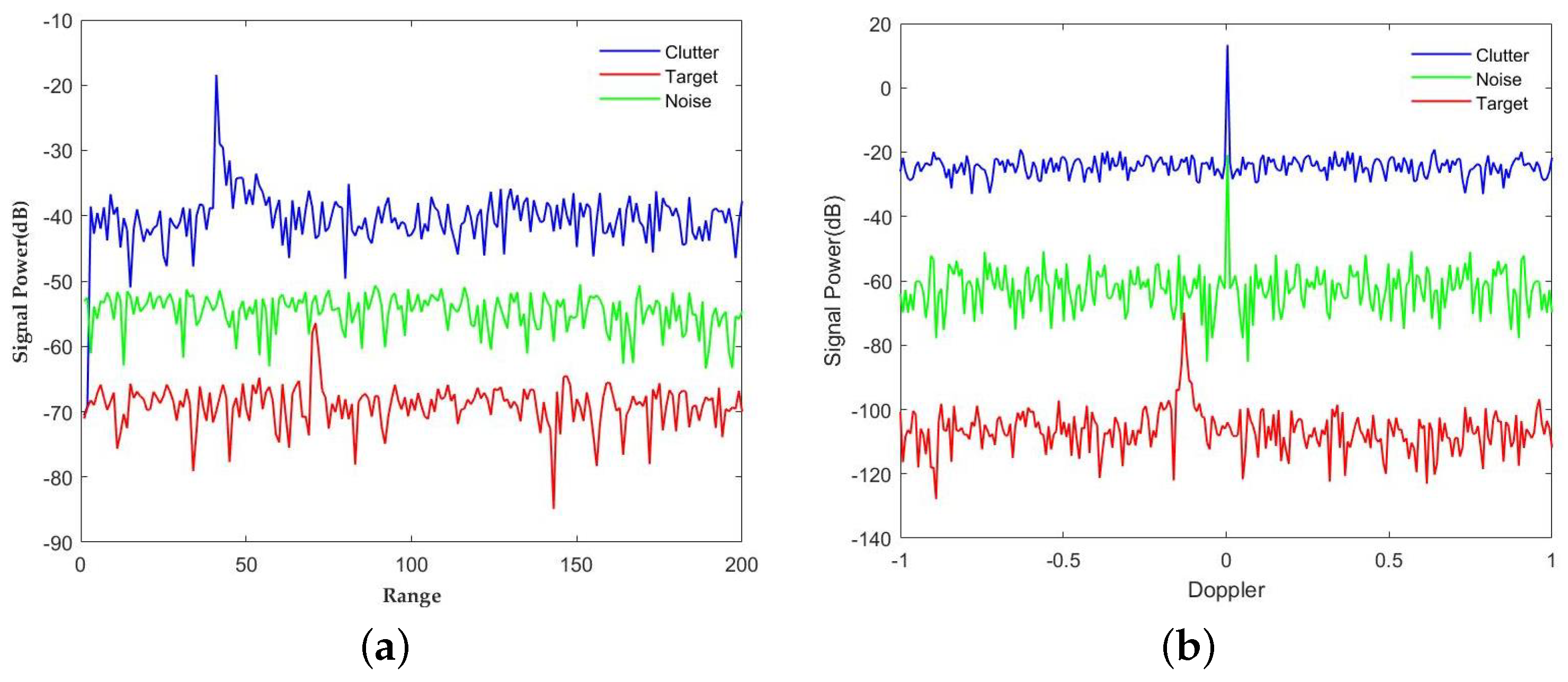
Radar echo signals often come accompanied by clutter, alongside the desired target signal. Clutter refers to unwanted interference signals that become entangled during signal processing or communication, unrelated to the intended signals. Since clutter is an inherent presence, it necessitates the adoption of clutter suppression techniques [11]. In this paper, we focus on investigating the shadowing effect in radar, as depicted in Figure 1. The diagram illustrates clutter echoes, noise echoes, and target signal echoes. As seen in Figure 1, clutter signals typically exhibit higher energy than the target signals, both in the range and Doppler domains. The direct processing of echo signals can induce signal distortion and errors, thereby compromising signal quality and significantly impacting the accuracy of target detection outcomes. Therefore, clutter suppression is of the utmost importance and deserves dedicated attention in radar target detection.
Significant efforts have been made by researchers in the development of clutter suppression techniques. Existing clutter suppression methods can be broadly categorized into two modes [12]: single−channel methods and multi−channel methods.
Early single−channel clutter suppression algorithms relied on classical linear filters, including average filters [13], median filters [14], and Kalman filters. These approaches primarily mitigated clutter by filtering the radar signal. As radar technology advanced, novel clutter suppression algorithms emerged, including nonlinear filters like wavelet transform and wavelet packet transform [15], which exhibit superior capability in handling nonlinear clutter and enhancing clutter suppression performance. Adaptive filters, like the least mean square (LMS) algorithm [16] and the recursive least squares (RLS) algorithm [17], adapt filter parameters based on clutter, enhancing clutter suppression capabilities. Classical single−channel clutter suppression techniques include moving target indication (MTI) [18] and moving target detection (MTD) [19], both based on the principle that the Doppler frequency shift of the echo signal varies with the target’s speed. These methods, including three-pulse canceller (TPC) [20,21], staggered pulse canceller (SPC) [20,22], and adaptive MTI methods [23], exploit the Doppler frequency shift characteristics of fixed clutter and moving target echo signals to extract and separate moving targets from stationary ground clutter and slow−moving clutter. Consequently, the removal of intense clutter and the extraction of target information are achieved [24]. TPC [20] is a classic clutter suppression technique that enhances radar target detection by canceling static clutter using the amplitudes of three consecutive pulses. SPC [22] is another common clutter suppression technique that improves radar sensitivity to moving targets by phase-shifting adjacent pulses to cancel static clutter. Vector averaging canceller (VAC) [13] is a clutter suppression method that utilizes statistical averaging to mitigate static clutter and highlight moving target signals in radar data. It is worth noting that since clutter exhibits motion, its Doppler frequency will not be zero [24]. Attempting to suppress clutter by forming a filter notch at zero frequency would fail to yield the desired outcome.
To overcome the limitations of single−channel clutter suppression methods, multi−channel technology has received significant attention, leading to the development of multi−channel clutter suppression techniques. Among these, displaced phase center antenna (DPCA) [25,26] and space-time adaptive processing (STAP) [27] have emerged as highly effective and popular approaches. DPCA mitigates clutter by eliminating the echo data received by two channels when their equivalent phase centers coincide. However, strict DPCA conditions must be satisfied regarding platform velocity, channel spacing, and pulse repetition frequency (PRF) [26]. Nevertheless, as the transmitter and receiver reside on separate platforms, the equivalent phase centers cannot align at the same location after a constant time interval. In the case of STAP, this method effectively suppresses clutter by creating a set of space-time two-dimensional joint filters. Accurate estimation of the clutter-impulse-noise covariance matrix (CNCM) is critical for successful STAP implementation. The maximum likelihood-based STAP algorithm estimates the CNCM using samples around the cell under test (CUT), assuming independent and identically distributed (i.i.d.) conditions. To ensure that the system performance loss remains below 3 dB, the samples employed for CNCM estimation should not be less than twice the system degrees of freedom (DOFs) [28]. Regrettably, obtaining a sufficient number of i.i.d. training samples poses considerable challenges in practice due to terrain constraints, antenna configuration, and other factors.
Numerous researchers have dedicated significant efforts to address challenges associated with clutter suppression. Despite advancements, three primary challenges persist within conventional methods. Firstly, traditional algorithms unavoidably result in the loss of signal energy while suppressing clutter. Secondly, these algorithms heavily rely on prior knowledge of the system and environment to enhance their performance. Lastly, when the Doppler spectrum of the target signal is entirely engulfed by clutter, the effectiveness of conventional clutter suppression techniques is significantly compromised.
To address these challenges, we introduce blind source separation (BSS) technology for radar clutter suppression [29]. BSS originates from the well-known “cocktail party effect” problem [30], which involves extracting target signals from noise without prior information. Its aim is to separate different sounds from mixed audio signals received by multiple sensors [31]. From the perspective of radar signal processing, this process is essentially the same as clutter suppression in radar systems. In this paper, based on the BSS algorithm, we design a clutter suppression scheme. Among the BSS algorithms, the parallel principal skewness analysis (PPSA) algorithm [32] is a well-established method. The scheme initially utilizes the PPSA algorithm to process the echoes in the range domain, identifying the positions of moving targets. Subsequently, the PPSA algorithm is applied once more to process the moving targets in the Doppler domain, determining their relative velocities. Compared to traditional clutter suppression methods, the proposed scheme exhibits superior clutter suppression performance, especially when clutter completely masks the Doppler spectrum of the target signal. Furthermore, the proposed scheme separates clutter from the targets, reducing the energy loss in the target signal.
The structure of this paper is as follows: Section 2 introduces the signaling model, blind source separation, and principles of PPSA, along with a detailed elaboration of the proposed clutter suppression scheme. Section 3 presents extensive experiments using simulated and real data to comprehensively evaluate the performance of the proposed scheme. Finally, Section 4 summarizes the findings and conclusions of this research endeavor.
2. Model and Method
2.1. Radar Echo Signal Model
Here, we primarily address narrowband pulse Doppler radar systems. We consider a monostatic radar configuration and a moving target scenario. The radar transmits multiple pulses after sinusoidal modulation and then receives the echo from the target after a certain time delay. The Doppler frequency of the received signal is calculated within the range of the received pulses sampled at the pulse repetition interval (PRI). Additionally, we assume that the radar beamwidth is wide enough to cover the entire size of the target, and the target’s velocity is considered constant within the data collection interval. Under these assumptions, the received signal can be expressed as follows:
where represents the reflection amplitude of the target, represents the Doppler frequency, and n represents the number of pulses. The clutter component is modeled using a moving-average model with independent and identically distributed sources as shown below:
and have zero-mean uniform distributions, where is defined as , with determining the slope of the window, and and L representing the Doppler center frequency and the length of the moving window of . Note that (2) approximates the spectral density of clutter as a compound Gaussian distribution, whose statistical correlation with actual clutter signals has been verified in [33].
Typically, the echo signal can be regarded as a linear combination of the transmitted signal and clutter. Additionally, there may be common additive noise present during the reception process. Therefore, the observed signal can be represented by the following matrix equation:
where represents the observed signal, denotes the source matrix consisting of the transmitted signal and clutter, is the mixing matrix, and signifies the additive noise matrix.
2.2. Blind Source Separation
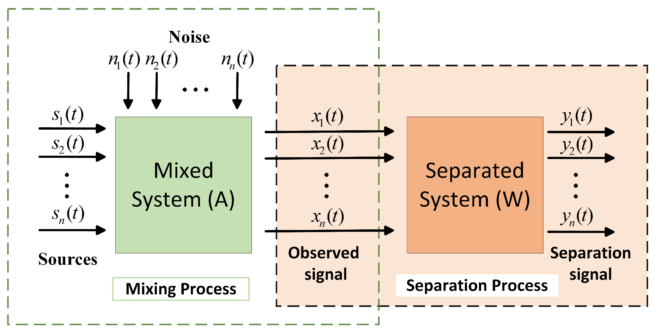
BSS involves reconstructing unobserved sources, such as time series and images, from a set of observed signals [34,35]. The term “blind” suggests that separation relies solely on the mixed signals, without prior knowledge of the individual sources or the mixing system. BSS is applied across various fields, including audio and speech signal separation [36], biomedical signal analysis [37], digital communication [38], image recovery [39,40], denoising [41], feature extraction [42], machine learning [43], and geophysical prospecting [44].
Given n independent source signals incident on M receiver units without considering time delay, the mixed signal received by each receiver unit can be expressed as a linear combination of the n source signals [40]. This mixed-signal model is represented by the equation:
where represents the statistically independent source signals, and denotes the observed signals received by the sensor after passing through the mixing system and being superimposed with noise. The matrix has dimensions , and represents the noise that is statistically independent from the source signals during the mixing process. The estimated signals are obtained by applying the separation matrix to the observed signals, where is an dimensional matrix. Thus, the vector of estimated source signals can be expressed as:
The goal of BSS is to determine a separation matrix of size , capable of extracting the source signals from the observed signals following a specific transformation, even in the absence of prior knowledge about the source signals and the mixing matrix . This facilitates obtaining the most accurate estimate of the source signals. A block diagram illustrating the BSS process is presented in Figure 2.
In radar systems, the echo signal can be considered a linear combination of target, noise, and clutter data [11]. The objective of clutter suppression is to separate the radar’s target signal from the combined data. On the other hand, BSS techniques can extract the desired signals from mixed signals and effectively achieve noise reduction [30]. Therefore, we introduce BSS technology to address the challenges faced by traditional clutter suppression algorithms.
2.3. Parallel Principal Skewness Analysis
Among the BSS algorithms, the PPSA algorithm [32] provides more accurate solutions and faster convergence. The PPSA algorithm flowchart is shown in Figure 3. The PPSA algorithm aims to de-average and whiten the observed signal initially, followed by the construction and solution of the co-skewness tensor to separate the matrix. Ultimately, the PPSA algorithm estimates the source signal.
Among the BSS algorithms, the PPSA algorithm [32] provides more accurate solutions and converges faster. The PPSA algorithm flowchart is depicted in Figure 3. The PPSA algorithm aims to de-average and whiten the observed signal initially. Then, it constructs and solves the co-skewness tensor to separate the matrix. Ultimately, the PPSA algorithm estimates the source signal.
(1) De-averaging: Assume that the observed data are , where is an vector, and N denotes the number of samples. De-averaging the data represents a fundamental preprocessing step. During this process, the average value of the signal is subtracted from each observed signal value, resulting in a zero-mean observed signal. Therefore, , with denoting the mean value, and representing the averaged data.
(2) Whitening: The purpose of the whitening process is to eliminate the second-order correlation present in each observed signal. Typically, the whitened signal exhibits improved convergence and algorithm stability compared to the unwhitened signal. The data should satisfy , where denotes the whitened data, is denoted as the whitening operator, while stands for the matrix of eigenvectors of the covariance matrix , and corresponds to the diagonal matrix of eigenvalues. In this context, is defined as .
(3) Constructing a co-skewness tensor: In the PPSA algorithm, constructing a co-skewness tensor resembles the construction of a covariance matrix in principal component analysis (PCA). PCA is based on second-order correlation statistical features to identify a set of orthogonal vectors that represent the original signal in terms of least squares. On the other hand, the PPSA algorithm performs a statistical analysis of third-order skewness on the data to maximize non-Gaussian components and separate independent signal sources. The co-skewness tensor is calculated using
where the “∘” symbol denotes the outer product of two vectors. Clearly, the co-skewness tensor is a supersymmetric tensor of size .
(4) Solve the eigenpairs of the co-skewness tensor: The computation of data skewness in any direction can be achieved by
Here, is a unit vector, and . So, the optimized model is
Then, (8) can be solved using the Lagrangian method:
The fixed-point method is employed to compute the value of each for every unit, which can be mathematically expressed as follows:
In the presence of a fixed point, the resultant solution is referred to as the first principal skewness direction. Here, represents its associated skewness value. This pairing of the eigenvalue and eigenvector, denoted as , was introduced in the field of tensor analysis by Lim [45] and Qi [46]. This process is then repeated to acquire a total of L eigenpairs, following the established methodology.
(5) Source signal separation: The output transformation matrix is represented as , facilitating the extraction of the separated signal .
2.4. The Proposed Clutter Suppression Scheme
Based on the PPSA algorithm, we designed a clutter suppression scheme. The scheme’s flowchart is shown in Figure 4. Initially, the PPSA algorithm is applied to process the echoes in the range domain, allowing for the localization of moving targets. Subsequently, the same PPSA algorithm is utilized to process the moving targets in the Doppler domain, enabling the calculation of their relative velocities.
The specific process of clutter suppression using this scheme is outlined as follows:
- (1)
- Assuming the size of the echo signal matrix is , where L and N represent the number of pulses and distance sampling points, respectively.
- (2)
- We perform whitening on the echo signal to obtain matrix (). Subsequently, based on , we construct the co-skewness tensor () and solve for its eigenvectors to obtain the separation matrix (). Finally, through the operation , we obtain the separated signal matrix ().
- (3)
- We utilize the classical CFAR algorithm to detect targets in the separated signal matrix to determine the target’s position, assuming the target position is .
- (4)
- If the Doppler spectrum of moving targets is obscured by clutter, we employ a similar approach to that used in the range domain. Specifically, we apply PPSA to the Doppler domain, followed by FFT transformation to extract the target’s relative velocity. The specific steps are as follows: first, we obtain the data , where is of size , with m representing the number of reference pulses. We can either directly select data around the target area or choose data with a higher correlation to the target. Then, we repeat the second step to obtain the separated signal matrix and subsequently perform FFT transformation to determine the target’s relative velocity.
2.5. Algorithm Complexity Analysis
This section theoretically analyzes the computational complexity of the proposed method, which primarily consists of three parts: (1) data whitening; (2) computation of high-order statistical tensors; and (3) computation of feature pairs. Assuming we extract p independent components from data of size , the complexity of data whitening is , the complexity of computing co-skewness tensors is , and the complexity of computing feature pairs is , where k is the average number of iterations. Therefore, the computational complexity of the proposed method is . The main advantage of the PPSA algorithm lies in its parallelism, allowing parallel computing to improve the algorithm’s execution speed. According to subsequent speed comparison experiments, it is evident that the PPSA algorithm achieves faster execution speed when handling high-dimensional data with parallel accelerated computation.
3. Experiment and Results Analysis
This section presents simulated and measured data experiments to validate the effectiveness of the proposed clutter suppression scheme. A comprehensive comparison is conducted between the proposed scheme and classical clutter suppression methods. To visually assess the clutter suppression performance of each algorithm, we applied constant false alarm rate (CFAR) detection to the output of each algorithm. Here, we utilized a CFAR configuration with a false alarm probability of , a guard cell size of 3, and a reference cell size of 10. For objective evaluation of the algorithm performance, we quantified the clutter suppression effect using the signal-to-clutter ratio (SCR). Due to the fact that clutter energy far exceeds noise energy in echo signals, we chose the SCR as the evaluation criterion. SCR is defined as the ratio of the square of the target signal amplitude to the average square amplitude of the clutter echoes. Mathematically, SCR is expressed as:
Here, denotes the amplitude of the target signal, and E[∗] represents the expectation operator. The clutter suppression effects are evaluated based on SCR. All algorithms were implemented on a laptop computer with an AMD Ryzen 7 5800H CPU, 16 GB RAM, operating at a frequency of 3.20 GHz, and utilizing MATLAB R2021a for execution.
3.1. Simulation Experiment
In this section, we first validate the effectiveness of the proposed scheme using simulated data. To simulate real-world scenarios, we generated radar echo data based on the parameters specified in Table 1, which describe the radar system. Additionally, we created moving targets by incorporating the motion target parameters outlined in Table 2. For the clutter signal, we utilized a simple clutter model called the constant gamma model, where we set the gamma value to −20 dB. This value is representative of the typical clutter found in a flat terrain. Finally, we conducted a comprehensive simulation and analysis, utilizing 40 received pulses and employing the aforementioned radar system and motion target parameters.
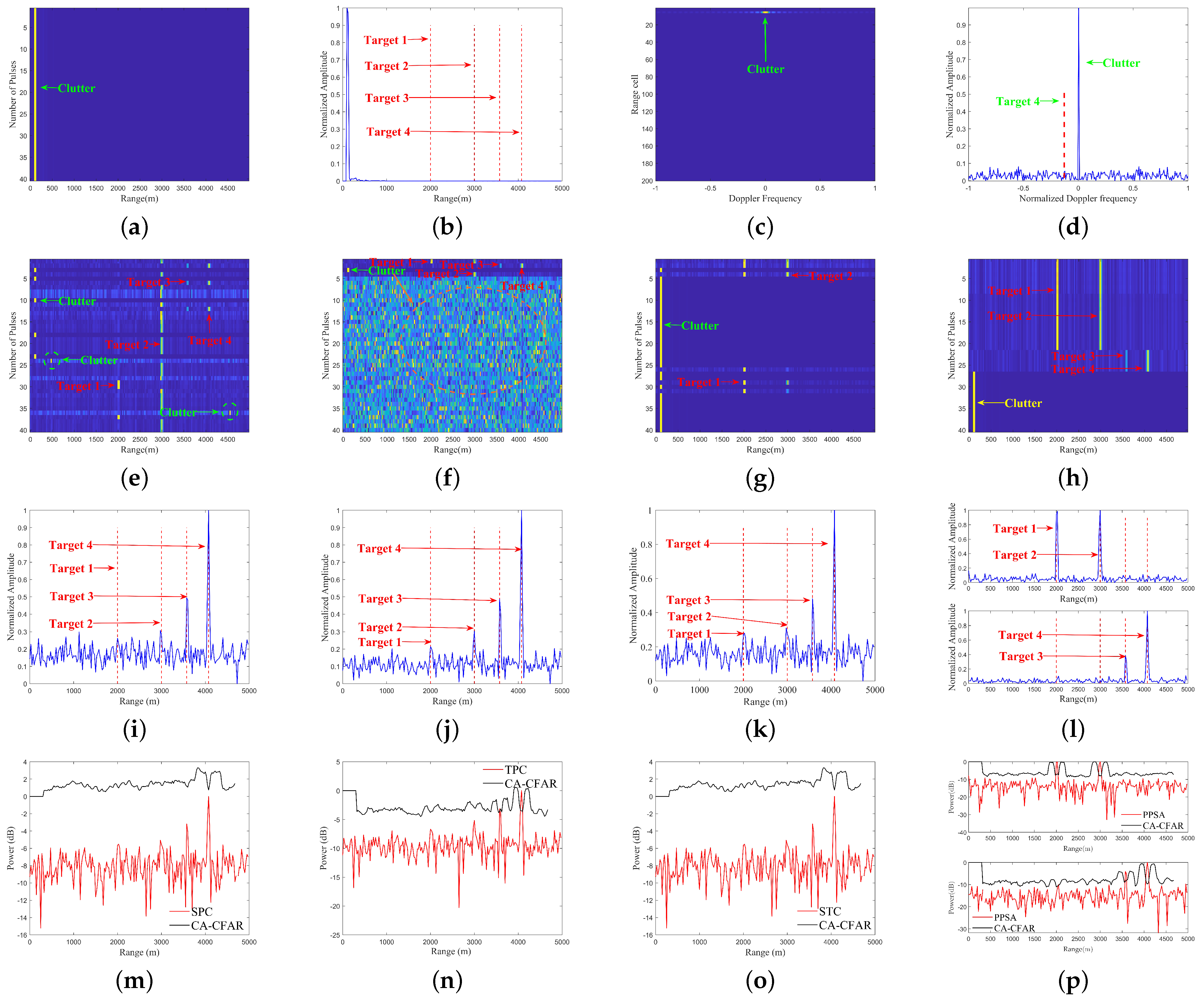
TPC [20], SPC [22], and VAC [13] are mature clutter suppression algorithms widely used in radar signal processing. FastICA [47], PSA [32], and NPSA [48] are classical BSS algorithms. We conducted comparative experiments using these algorithms and the proposed scheme. For the sake of convenience in description, we can use RD−PPSA to refer to the proposed scheme. The experimental results are shown in Figure 5.
From Figure 5a–d, it can be found that before applying any clutter suppression algorithms, the targets are obscured by clutter signals in both the range and Doppler domains. Without any processing, effective target detection is challenging. Figure 5e–h show the results of the BSS algorithms. It can be observed that the BSS methods are capable of separating targets from strong clutter interference. However, the separation results obtained by FastICA and PSA still contain significant clutter interference, especially in the case of the PSA algorithm. The NPSA algorithm can cleanly and effectively separate target 1 and target 2, but it fails to separate target 3 and target 4. In contrast, RD−PPSA can accurately and cleanly separate targets from clutter. In addition, we also compared the computational speed of these different BSS algorithms by comparing the average computing time of 50 runs, as shown in Table 3. Table 3 shows that RD−PPSA has the lowest runtime. Figure 5i–l illustrate the clutter suppression results using SPC, TPC, VAC, and RD−PPSA. From the figures, significant peaks can be observed at the locations of target 3 and target 4 for SPC, TPC, and VAC algorithms. However, significant clutter is still present at the positions of target 1 and target 2. In comparison, RD−PPSA exhibits distinct peaks at all target positions. Figure 5m–p present the CFAR detection results for these algorithms. It can be identified that the SPC, TPC, and VAC algorithms fail to effectively detect target 1 and target 2, while RD−PPSA successfully detects all targets.
Typical Doppler radar algorithms use FFT to determine the relative velocity of targets. After determining the target’s position, we used FFT to determine the target’s relative velocity. It is worth noting that for the determination of the target’s relative velocity, we processed 256 pulses. This is because target 1 and target 2 have very small velocities and clutter and noise are concentrated at zero frequency. To clearly distinguish the two frequencies, a sufficient number of pulses are needed. We conducted experiments using FFT and RD−PPSA, and the experimental results are shown in Figure 6.
From Figure 6a, it can be noticed that due to frequency aliasing, and clutter interference, the Doppler spectrum of moving targets is often submerged in the clutter and noise’s Doppler spectrum. In this case, direct application of the traditional FFT-CFAR method cannot effectively detect the target. Figure 6b–d show the results of RD−PPSA processing. After RD−PPSA processing, targets previously obscured by clutter and noise become fully visible.
To objectively evaluate the performance of the algorithms, we compared the SCR of different clutter suppression algorithms, and the evaluation metrics are listed in Table 4. These results demonstrate that RD−PPSA significantly improves the SCR after processing of the echoes where the target’s Doppler spectrum is covered by clutter. This result indicates that RD−PPSA achieves the highest SCR when dealing with situations where the Doppler spectrum of the target is obscured by clutter. It significantly improves the SCR compared to traditional clutter suppression methods.
Validating the algorithm’s effectiveness involved conducting the detection probability tests for TPC, SPC, VAC, and RD−PPSA across different SNR levels. With a false alarm probability of and 40 pulses, we performed 1000 Monte Carlo simulations, and the resulting detection outcomes for TPC, SPC, VAC, and RD−PPSA are depicted in Figure 7. These results highlight the superior performance of RD−PPSA over others at varying SNR levels, especially when SNR is below 5 dB, significantly improving detection performance.
To verify the loss of target signal energy during clutter suppression, we evaluated the target detection probability of different algorithms at various velocities, ranging from 0 to 14 m/s with a step size of 1 m/s. The results are shown in Figure 8. The research results indicate that when the target’s Doppler frequency is close to a zero frequency (where the clutter’s Doppler frequency is located), traditional clutter suppression algorithms inevitably suppress the target’s energy while suppressing clutter. In contrast, RD−PPSA employs a separation approach for clutter suppression, which better preserves the target signal energy compared to other methods.
3.2. Multi−Channel Radar Target Detection Experiment
To validate the efficacy of the RD−PPSA algorithm in suppressing clutter for multi−channel targets, this section focuses on applying the RD−PPSA algorithm to address the issue of Doppler spectrum clutter in such scenarios. We simulate a narrowband pulse Doppler airborne radar system with a positive aspect angle, and the key simulation parameters are presented in Table 5. A uniform linear array antenna is employed for the simulations. The clutter is modeled using a constant gamma model with a gamma value of −15 dB, which is suitable for simulating terrain covered with trees. We define a non-fluctuating target moving on the ground, and the target parameters are specified in Table 6.
The experimental setup for the simulation data is as follows. Radar echo data are generated based on the radar system parameters listed in Table 5. It is important to note that a six-element uniform linear array antenna is used for radar transmission and reception signals, with the antenna element spacing set to half the wavelength of the waveform. The total number of received signals includes return signals from the combination of targets, clutter, noise, and interference. Finally, we simulate 10 receiving pulses using the radar system and moving target parameters. The resulting signal forms a data cube with dimensions of 200 × 10 × 6. We conducted experiments using the FastICA, PSA, NPSA, ADPCA, SMI, Optimal−STAP and the RD−PPSA algorithm in this paper. The experimental results are shown in Figure 9.
Figure 9a–d demonstrate that the target is submerged within clutter signals in both the range and Doppler domains. Figure 9a reveals that due to the high-speed motion of the radar platform, clutter echoes occupy not only the zero Doppler but also other Doppler spectra. Clutter manifests as a diagonal line in the two-dimensional angle–Doppler plane, while received interference signals appear as white noise propagating across the entire Doppler spectrum at a specific angle (approximately 120 degrees). Without further processing, effective target detection becomes challenging.
Observing Figure 9e–h, we can see that the BSS method effectively separates targets from clutter, whereas there is noticeable interference in the results obtained by FastICA, PSA, and NPSA. In contrast, the RD−PPSA algorithm achieves the accurate separation of targets from clutter, demonstrating outstanding separation effectiveness. In Figure 9i–l, although ADPCA and SMI algorithms exhibit significant peaks at the positions of targets, there is still a considerable amount of clutter. Conversely, the Optimal−STAP and RD−PPSA algorithms show distinct peaks at all target positions, with less clutter near the targets in the PPSA results. Additionally, Figure 9m–p demonstrate that ADPCA and SMI fail to effectively detect targets, whereas the Optimal−STAP algorithm and RD−PPSA method successfully detect the targets.
Table 7 provides evaluation criteria for the various clutter suppression algorithms. The results demonstrate that the RD−PPSA algorithm achieves the highest SCR and outperforms other clutter suppression methods in terms of clutter suppression effectiveness.
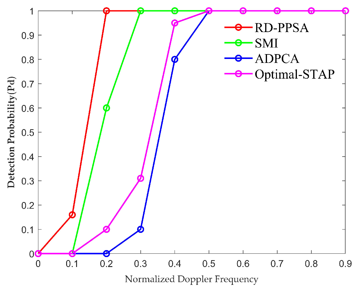
To further assess the algorithm’s efficacy, we conducted tests to determine the detection probabilities of the ADPCA, SMI, Optimal−STAP, and RD−PPSA algorithms under different SCR levels. The false alarm probability was set to 10−3, and a total of 30 pulses were used. The detection results for each algorithm are depicted in Figure 10. The test results indicate that the RD−PPSA algorithm significantly improves detection performance, particularly when the SCR is below −30 dB, compared to other methods.
To evaluate the loss of target signal energy during clutter suppression, we examined the target echo energy loss of each algorithm at different Doppler frequencies. The detection results for each algorithm are shown in Figure 11. These results indicate that while other methods inevitably suppress the energy of the target signal while suppressing clutter, the RD−PPSA algorithm better preserves the energy of signals near zero frequency.
Based on the analysis and results of these experiments, it is evident that the RD−PPSA algorithm is effective in scenarios where the Doppler spectrum of multi−channel targets is submerged by clutter. All targets can be detected, and the SCR of each target is significantly improved.
3.3. Real Data Experiment
In this section, we verify the effectiveness of the RD−PPSA algorithm using “A dataset for detection and tracking of dim aircraft targets through radar echo sequences” [49]. The main facilities and equipment used for data collection were high towers and a rotating platform, which were located in Meixian, Baoji City, Shanxi Province, China. The servo radar sensor was mounted on the rotating platform installed on a tower approximately 90 m above the ground. The narrow−beam radar was fixed to the platform’s edge at a specific angle. The data collection employed a Ka−band general purpose recording device, and its basic performance parameters are listed in Table 8. It should be noted that other BSS algorithms often encounter varying degrees of clutter in both the range and Doppler domains, making it challenging to accurately separate clutter from target signals. Therefore, in this section, we only present the processing results of the RD−PPSA algorithm.
3.3.1. Experiment 1: The Target Is Located in Different Distance Cells
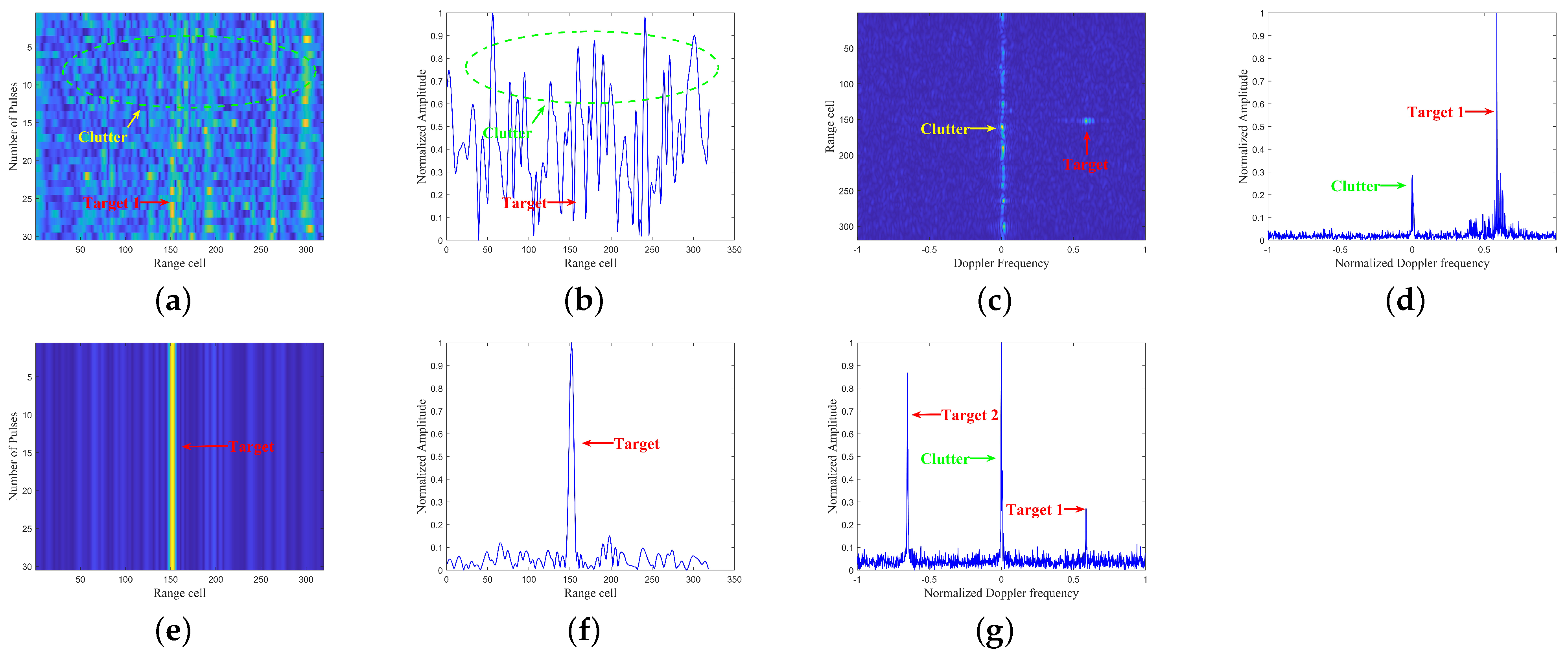
Here, we use “data 1” for data experiments. It is worth noting that this dataset contains a total of 64,000 pulses, and RD−PPSA belongs to the category of short-term clutter suppression. Therefore, we choose an initial 30 pulses in the 0–50 ms time interval for the experiment. At this time, target 1 is located in the 151st range cell, and target 2 is located in the 72nd range cell. We use the proposed scheme for data processing. The experimental results are shown in Figure 12.
From Figure 12a,b, it can be observed that there is significant clutter interference with the targets in the range domain. In Figure 12c,d, it can be seen that there is a considerable amount of interference around the Doppler spectrum of target 1, and the Doppler spectrum of target 2 is submerged in clutter. Figure 12e represents the result of clutter separation using RD−PPSA. It can be seen that RD−PPSA effectively separates the targets from clutter. Figure 12f displays the clutter suppression results in the range domain using RD−PPSA, showing distinct peaks at the positions of target 1 and target 2. After determining the target positions, FFT is utilized to determine the relative velocity of the targets. For velocity estimation, we processed 128 pulses. Directly applying the traditional FFT−CFAR method for target detection cannot accurately determine the relative velocity of the targets. Figure 12g,h show the results after processing with RD−PPSA. The results reveal that RD−PPSA processing effectively suppresses interference around target 1, revealing target 2, which was initially obscured by clutter.
To objectively evaluate the algorithm’s performance, we also compare the SCR under this dataset, and the quantitative results are shown in Table 9. The results clearly indicate a significant improvement in SCR with RD−PPSA.
3.3.2. Experiment 2: Targets in the Same Distance Cell
In this section, we utilize “data2" for experiments. We select the initial 30 pulses for experimentation, during which both target 1 and target 2 are located in the 151st range cell. We process the data using RD−PPSA, and the experimental results are shown in Figure 13.
From Figure 13a–d, it can be observed that there is a significant amount of clutter in both the range and Doppler domains, especially the Doppler spectrum of target 2, which is completely submerged in clutter. Effectively detecting target 2 without any processing presents a challenge. Figure 13e represents the result of clutter separation using RD−PPSA. It can be seen that RD−PPSA effectively separates the targets from clutter. In Figure 13f, it can be observed that RD−PPSA shows distinct peaks at the positions of the targets after algorithmic processing. After determining the target positions, we use FFT to determine the targets’ relative velocities. Figure 13g displays the results obtained using RD−PPSA. The results show that after processing, not only is the clutter around target 1 effectively suppressed but target 2, previously obscured by clutter, is also fully revealed.
To objectively evaluate the algorithm’s performance, we also compare the SCR under this dataset, and the quantitative results are shown in Table 10. The results indicate a significant improvement in the SCR for RD−PPSA.
Based on the experimental analysis presented above, it can be clearly observed that RD−PPSA effectively addresses the issue of targets being submerged in clutter in the range–Doppler domain.
4. Conclusions
To address challenges inherent in conventional clutter suppression methods, this paper introduces a clutter suppression scheme based on PPSA. Comparative analysis between the simulated and processed measured data confirms the scheme’s superior performance in clutter mitigation. The proposed scheme offers the following advantages: (1) independence from prior information, as eliminating the need for prior knowledge enhances versatility and applicability; (2) improved clutter suppression capabilities, especially when the clutter’s Doppler spectrum masks or overwhelms the target signal’s Doppler spectrum; and (3) efficient clutter and target separation with minimal energy loss, achieving effective separation while preserving target signal energy. Our focus is primarily on fixed clutter suppression, and we discuss a potential optimization model for extending the scheme’s applicability to various clutter types. Future work will explore this optimization model to broaden the scope of our clutter suppression approach.
Author Contributions
Conceptualization, D.W.; methodology, D.W.; software, D.W.; validation, D.W. and L.C.; formal analysis, D.W.; investigation, D.W., L.C. and C.W.; resources, D.W., L.C. and C.W.; data curation, D.W. and C.W.; writing—original draft preparation, D.W.; writing—review and editing, D.W., L.C. and C.W.; visualization, D.W., L.C. and C.W.; supervision, D.W., L.C. and C.W.; project administration, L.C. and C.W. All authors have read and agreed to the published version of the manuscript.
Funding
This research received no external funding.
Data Availability Statement
The specific website for the dataset “A dataset for detection and tracking of dim aircraft targets through radar echo sequences” is: http://www.csdata.org/p/386/ (accessed on 1 January 2023).
Conflicts of Interest
The authors declare no conflicts of interest.
References
- Marcum, J. A statistical theory of target detection by pulsed radar. IRE Trans. Inf. Theory 1960, 6, 59–267. [Google Scholar] [CrossRef]
- Ratches, J.A. Review of current aided/automatic target acquisition technology for military target acquisition tasks. Opt. Eng. 2011, 50, 072001. [Google Scholar] [CrossRef]
- Liu, Z.; Cai, Y.; Wang, H.; Chen, L.; Gao, H.; Jia, Y.; Li, Y. Robust target recognition and tracking of self-driving cars with radar and camera information fusion under severe weather conditions. IEEE Trans. Intell. Transp. Syst. 2021, 23, 6640–6653. [Google Scholar] [CrossRef]
- Prabaswara, A.; Munir, A.; Suksmono, A.B. GNU Radio based software-defined FMCW radar for weather surveillance application. In Proceedings of the 2011 6th International Conference on Telecommunication Systems, Services, and Applications (TSSA), Denpasar, Indonesia, 20–21 October 2011; IEEE: Piscataway, NJ, USA, 2011; pp. 227–230. [Google Scholar]
- Cao, C.; Zhang, J.; Meng, J.; Zhang, X.; Mao, X. Clutter suppression and target tracking by the low-rank representation for airborne maritime surveillance radar. IEEE Access 2020, 8, 160774–160789. [Google Scholar] [CrossRef]
- Zhang, J.A.; Rahman, M.L.; Wu, K.; Huang, X.; Guo, Y.J.; Chen, S.; Yuan, J. Enabling joint communication and radar sensing in mobile networks—A survey. IEEE Commun. Surv. Tutor. 2021, 24, 306–345. [Google Scholar] [CrossRef]
- Yan, J.; Liu, H.; Jiu, B.; Liu, Z.; Bao, Z. Joint Detection and Tracking Processing Algorithm for Target Tracking in Multiple Radar System. IEEE Sens. J. 2015, 15, 6534–6541. [Google Scholar] [CrossRef]
- Yan, B.; Paolini, E.; Xu, L.; Lu, H. A Target Detection and Tracking Method for Multiple Radar Systems. IEEE Trans. Geosci. Remote Sens. 2022, 60, 1–21. [Google Scholar] [CrossRef]
- Shi, C.; Dong, J.; Salous, S.; Wang, Z.; Zhou, J. Collaborative Trajectory Planning and Resource Allocation for Multi-Target Tracking in Airborne Radar Networks under Spectral Coexistence. Remote Sens. 2023, 15, 3386. [Google Scholar] [CrossRef]
- Fang, H.; Liao, G.; Liu, Y.; Zeng, C. Siam-sort: Multi-target tracking in video SAR based on tracking by detection and Siamese network. Remote Sens. 2022, 15, 146. [Google Scholar] [CrossRef]
- Conte, E.; Lops, M.; Ricci, G. Asymptotically optimum radar detection in compound-Gaussian clutter. IEEE Trans. Aerosp. Electron. Syst. 1995, 31, 617–625. [Google Scholar] [CrossRef]
- Yang, J.; Liu, C.; Wang, Y. Detection and imaging of ground moving targets with real SAR data. IEEE Trans. Geosci. Remote Sens. 2014, 53, 920–932. [Google Scholar] [CrossRef]
- Mahalanobis, A.; Kumar, B.V.; Casasent, D. Minimum average correlation energy filters. Appl. Opt. 1987, 26, 3633–3640. [Google Scholar] [CrossRef] [PubMed]
- Gallagher, N.; Wise, G. A theoretical analysis of the properties of median filters. IEEE Trans. Acoust. Speech Signal Process. 1981, 29, 1136–1141. [Google Scholar] [CrossRef]
- Carevic, D. Clutter reduction and target detection in ground-penetrating radar data using wavelets. In Proceedings of the Detection and Remediation Technologies for Mines and Minelike Targets IV, Orlando, FL, USA, 5–9 April 1999; SPIE: Bellingham, WA, USA, 1999; Volume 3710, pp. 973–978. [Google Scholar]
- Liu, W.; Pokharel, P.P.; Principe, J.C. The kernel least-mean-square algorithm. IEEE Trans. Signal Process. 2008, 56, 543–554. [Google Scholar] [CrossRef]
- Engel, Y.; Mannor, S.; Meir, R. The kernel recursive least-squares algorithm. IEEE Trans. Signal Process. 2004, 52, 2275–2285. [Google Scholar] [CrossRef]
- Ma, H.; Antoniou, M.; Pastina, D.; Santi, F.; Pieralice, F.; Bucciarelli, M.; Cherniakov, M. Maritime moving target indication using passive GNSS-based bistatic radar. IEEE Trans. Aerosp. Electron. Syst. 2017, 54, 115–130. [Google Scholar] [CrossRef]
- Xu, J.; Yu, J.; Peng, Y.N.; Xia, X.G. Radon-Fourier transform for radar target detection, I: Generalized Doppler filter bank. IEEE Trans. Aerosp. Electron. Syst. 2011, 47, 1186–1202. [Google Scholar] [CrossRef]
- Richards, M.A. Fundamentals of Radar Signal Processing; McGraw-Hill Education: New York, NY, USA, 2014. [Google Scholar]
- Cohen, I.; Levanon, N. Adjusting 3-pulse canceller to enhance slow radar targets. In Proceedings of the 2015 IEEE International Conference on Microwaves, Communications, Antennas and Electronic Systems (COMCAS), Tel-Aviv, Israel, 2–4 November 2015; IEEE: Piscataway, NJ, USA, 2015; pp. 1–5. [Google Scholar]
- Tuszynski, M.; Wojtkiewicz, A.; Klembowski, W. Bimodal clutter MTI filter for staggered PRF radars. In Proceedings of the IEEE International Conference on Radar, Arlington, VA, USA, 7–10 May 1990; IEEE: Piscataway, NJ, USA, 1990; pp. 176–180. [Google Scholar]
- Zhang, W.; Ma, S.; Du, Q. Optimization of adaptive MTI filter. Int. J. Commun. Netw. Syst. Sci. 2017, 10, 206–217. [Google Scholar] [CrossRef]
- McDonald, M.; Damini, A. Limitations of nonlinear chaotic dynamics in predicting sea clutter returns. IEE Proc.-Radar Sonar Navig. 2004, 151, 105–113. [Google Scholar] [CrossRef]
- Cerutti-Maori, D.; Sikaneta, I. A generalization of DPCA processing for multichannel SAR/GMTI radars. IEEE Trans. Geosci. Remote Sens. 2012, 51, 560–572. [Google Scholar] [CrossRef]
- Jung, J.H.; Jung, J.S.; Jung, C.H.; Kwag, Y.K. Ground moving target displacement compensation in the DPCA based SAR-GMTI system. In Proceedings of the 2009 IEEE Radar Conference, Pasadena, CA, USA, 4–8 May 2009; IEEE: Piscataway, NJ, USA, 2009; pp. 1–4. [Google Scholar]
- Ward, J. Space-time adaptive processing for airborne radar. In Proceedings of the 1995 International Conference on Acoustics, Speech, and Signal Processing, Detroit, MI, USA, 9–12 May 1995. [Google Scholar]
- Reed, I.S.; Mallett, J.D.; Brennan, L.E. Rapid convergence rate in adaptive arrays. IEEE Trans. Aerosp. Electron. Syst. 1974, 10, 853–863. [Google Scholar] [CrossRef]
- Cao, X.R.; Liu, R.W. General approach to blind source separation. IEEE Trans. Signal Process. 1996, 44, 562–571. [Google Scholar]
- Chen, X.; Wang, Z.J.; McKeown, M. Joint blind source separation for neurophysiological data analysis: Multiset and multimodal methods. IEEE Signal Process. Mag. 2016, 33, 86–107. [Google Scholar] [CrossRef]
- Holobar, A.; Farina, D. Noninvasive neural interfacing with wearable muscle sensors: Combining convolutive blind source separation methods and deep learning techniques for neural decoding. IEEE Signal Process. Mag. 2021, 38, 103–118. [Google Scholar] [CrossRef]
- Geng, X.; Ji, L.; Sun, K. Principal skewness analysis: Algorithm and its application for multispectral/hyperspectral images indexing. IEEE Geosci. Remote Sens. Lett. 2014, 11, 1821–1825. [Google Scholar] [CrossRef]
- Farina, A.; Russo, A. Radar detection of correlated targets in clutter. IEEE Trans. Aerosp. Electron. Syst. 1986, 22, 513–532. [Google Scholar] [CrossRef]
- Bousse, M.; Debals, O.; De Lathauwer, L. A tensor-based method for large-scale blind source separation using segmentation. IEEE Trans. Signal Process. 2016, 65, 346–358. [Google Scholar] [CrossRef]
- Taha, L.Y.; Abdel-Raheem, E. Blind Source Separation: A Performance Review Approach. In Proceedings of the 2022 5th International Conference on Signal Processing and Information Security (ICSPIS), Virtual, 7–8 December 2022; IEEE: Piscataway, NJ, USA, 2022; pp. 148–153. [Google Scholar]
- Taha, L.Y.; Abdel-Raheem, E. Efficient blind source extraction of noisy mixture utilising a class of parallel linear predictor filters. IET Signal Process. 2018, 12, 1009–1016. [Google Scholar] [CrossRef]
- Da Poian, G.; Bernardini, R.; Rinaldo, R. Separation and analysis of fetal-ECG signals from compressed sensed abdominal ECG recordings. IEEE Trans. Biomed. Eng. 2015, 63, 1269–1279. [Google Scholar] [CrossRef] [PubMed]
- Miyajima, T.; Teshiromori, H.; Sugitani, Y. Adaptive self-interference suppression for full duplex filter-and-forward relaying. IEEE Wirel. Commun. Lett. 2020, 9, 1701–1704. [Google Scholar] [CrossRef]
- Ourdou, A.; Ghazdali, A.; Metrane, A.; Hakim, M. Digital document image restoration using a blind source separation method based on copulas. IOP Proc. J. Physics Conf. Ser. 2021, 1743, 012034. [Google Scholar] [CrossRef]
- Chang, S.; Deng, Y.; Zhang, Y.; Zhao, Q.; Wang, R.; Zhang, K. An advanced scheme for range ambiguity suppression of spaceborne SAR based on blind source separation. IEEE Trans. Geosci. Remote Sens. 2022, 60, 1–12. [Google Scholar] [CrossRef]
- Feng, L.; Li, J.; Li, C.; Liu, Y. A Blind Source Separation Method Using Denoising Strategy Based on ICEEMDAN and Improved Wavelet Threshold. Math. Probl. Eng. 2022, 2022, 3035700. [Google Scholar] [CrossRef]
- Hyvarinen, A.; Karhunen, J.; Oja, E. Independent component analysis. Stud. Inform. Control 2002, 11, 205–207. [Google Scholar]
- Bhanot, A.; Meillier, C.; Heitz, F.; Harsan, L. Spatially constrained online dictionary learning for source separation. IEEE Trans. Image Process. 2021, 30, 3217–3228. [Google Scholar] [CrossRef] [PubMed]
- Liu, W.; Mandic, D.P.; Cichocki, A. A class of novel blind source extraction algorithms based on a linear predictor. In Proceedings of the 2005 IEEE International Symposium on Circuits and Systems (ISCAS), Kobe, Japan, 23–26 May 2005; IEEE: Piscataway, NJ, USA, 2005; pp. 3599–3602. [Google Scholar]
- Lim, L.H. Singular values and eigenvalues of tensors: A variational approach. In Proceedings of the 1st IEEE International Workshop on Computational Advances in Multi-Sensor Adaptive Processing, Puerto Vallarta, Mexico, 13–15 December 2005; IEEE: Piscataway, NJ, USA, 2005; pp. 129–132. [Google Scholar]
- Qi, L. Eigenvalues of a real supersymmetric tensor. J. Symb. Comput. 2005, 40, 1302–1324. [Google Scholar] [CrossRef]
- Oja, E.; Yuan, Z. The FastICA algorithm revisited: Convergence analysis. IEEE Trans. Neural Netw. 2006, 17, 1370–1381. [Google Scholar] [CrossRef] [PubMed]
- Geng, X.; Wang, L. NPSA: Nonorthogonal principal skewness analysis. IEEE Trans. Image Process. 2020, 29, 6396–6408. [Google Scholar] [CrossRef] [PubMed]
- Song, Z.; Hui, B.; Fan, H.; Zhou, J.; Zhu, Y.; Da, K.; Zhang, X.; Su, H.; Jin, W.; Zhang, Y.; et al. A dataset for detection and tracking of dim aircraft targets through radar echo sequences. China Sci. Data 2020, 5, 3. [Google Scholar]
Figure 1.
The problem of masking. (a) Masking effect in the distance domain. (b) Masking effect in the Doppler domain.
Figure 1.
The problem of masking. (a) Masking effect in the distance domain. (b) Masking effect in the Doppler domain.

Figure 2.
Block diagram illustrating the BSS process.

Figure 3.
PPSA algorithm flowchart.

Figure 4.
The clutter suppression scheme flowchart.

Figure 5.
The simulated data echo characteristics as well as the clutter suppression and CFAR detection results using different algorithms. (a) Overall echo signal. (b) Single pulse echo. (c) Range–Doppler plot of the data. (d) Target’s Doppler plot. (e) Separation result using FastICA. (f) Separation result using PSA. (g) Separation result using NPSA. (h) Separation result using RD−PPSA. (i) Clutter suppression result using SPC. (j) Clutter suppression result using TPC. (k) Clutter suppression result using VAC. (l) Clutter suppression result using RD−PPSA. (m) Detection result using SPC CFAR. (n) Detection result using TPC CFAR. (o) Detection result using VAC CFAR. (p) Detection result using RD−PPSA CFAR.

Figure 6.
The target Doppler characteristics and the Doppler results of the target after being processed by RD−PPSA. (a) Doppler of target before the algorithm processing. (b) Doppler result of target 1 after separation by RD−PPSA. (c) Doppler result of target 2 after separation by RD−PPSA. (d) Doppler result of Targets 3 and 4 after separation by RD−PPSA.

Figure 7.
Detection probability of each algorithm under different SNR.

Figure 8.
Detection probability of each algorithm at different Doppler frequencies.

Figure 9.
The original signal affected by clutter, and the results after being processed by different algorithms. (a) Overall echo signal. (b) Single−pulse echo. (c) Echo–power spectrum. (d) Echo–Doppler spectrum. (e) Separation result using FastICA. (f) Separation result using PSA. (g) Separation result using NPSA. (h) Separation result using RD−PPSA. (i) Clutter suppression result using ADPCA. (j) Clutter suppression result using SMI. (k) Clutter suppression result using Optimal−STAP. (l) Clutter suppression result using PPSA. (m) Detection result using ADPCA CFAR. (n) Detection result using SMI CFAR. (o) Detection result using Optimal−STAP CFAR. (p) Detection result using RD−PPSA CFAR.

Figure 10.
Detection probability of each algorithm under different SCNR.

Figure 11.
The target echo energy loss for each algorithm at different Doppler frequencies.

Figure 12.
The echo characteristics of data 1, as well as the clutter suppression and CFAR detection results obtained using different algorithms. (a) Overall echo signal. (b) Single pulse echo. (c) Range–Doppler plot of the data. (d) Target’s Doppler plot. (e) Separation result using RD−PPSA. (f) Clutter suppression results in the range domain using RD−PPSA. (g) Doppler result of target 1 using RD−PPSA. (h) Doppler result of target 2 using RD−PPSA.

Figure 13.
The echo characteristics of data 2, as well as the clutter suppression and CFAR detection results obtained using different algorithms. (a) Overall echo signal. (b) Single pulse echo. (c) Range–Doppler plot of the data. (d) Target’s Doppler plot. (e) Separation result using RD−PPSA. (f) Clutter suppression results in the range domain using RD−PPSA. (g) Doppler results of Target by RD−PPSA.


Table 1.
Simulated radar system parameters.
| Parameter | Numerical Value |
|---|---|
| pulse repetition frequency (Hz) | 3000 |
| radar wavelength (m) | 0.03 |
| pulse train length | 200 |
| radar operating frequency range (GHz) | 5–15 |
| antenna height (m) | 100 |
| bandwidth | 3 M |
| sampling rate | 6 M |
| receiver gain (dB) | 20 |
Table 2.
Simulated movement target parameters.
| Parameter | Target 1 | Target 2 | Target 3 | Target 4 |
|---|---|---|---|---|
| Range (m) | 2000.6 | 3000.2 | 3575.5 | 4075.3 |
| RCS (m2) | 2.0 | 10.0 | 2.0 | 10.0 |
| V (m/s) | −5.0 | 5.0 | 30.0 | 30.0 |
Table 3.
Evaluation of average running time for different BSS algorithms over 40 pulses.
| Method | FastICA | PSA | NPSA | RD−PPSA |
|---|---|---|---|---|
| Time (s) | 2.5466 | 15.6284 | 17.5896 | 1.7335 |
Table 4.
SCR for different clutter suppression algorithms under simulated data.
| Algorithms | Target 1 | Target 2 | Target 3 | Target 4 |
|---|---|---|---|---|
| Original Signal | −42.7049 | −34.8377 | −40.7049 | −33.6546 |
| SPC | 4.8807 | 6.0262 | 9.8141 | 16.1766 |
| TPC | 5.7487 | 8.8759 | 12.9558 | 19.2355 |
| VAC | 7.1816 | 9.2411 | 14.4230 | 20.3727 |
| RD−PPSA | 26.5150 | 26.7827 | 21.2409 | 29.4732 |
Table 5.
Radar system parameters.
| Parameter | Numerical Value |
|---|---|
| pulse repetition frequency (Hz) | 50,000 |
| radar wavelength (Hz) | 0.0749 |
| pulse train length | 200 |
| radar operating frequency range (GHz) | 4 |
| antenna height (m) | 3000 |
| aircraft speed (m/s) | 240 |
| sampling rate | 1 M |
Table 6.
Movement target parameters.
| Parameter | Range (m) | RCS (dB) | V (m/s) |
|---|---|---|---|
| Target | 1735.5 | 0.75 | 2.00 |
Table 7.
Relative running time of the considered filters.
| Algorithms | Original Signal | ADPCA | SMI | Optimal−STAP | RD−PPSA |
|---|---|---|---|---|---|
| Target (dB) | −34.2358 | 5.2465 | 12.2465 | 26.2362 | 28.2683 |
Table 8.
Radar system parameters.
| Parameter | Numerical Value |
|---|---|
| Radar carrier frequency (Hz) | 35 G |
| Pulse repetition rate (Hz) | 32 K |
| Pulse train length (m) | 1.875 |
Table 9.
SCR for different clutter suppression algorithms under data1.
| Algorithms | Original Signal | RD−PPSA |
|---|---|---|
| Target1 SCR | 8.5773 | 25.2244 |
| Target2 SCR | 2.6160 | 18.8695 |
Table 10.
SCR for different clutter suppression algorithms under data2.
| Algorithms | Original Signal | RD−PPSA |
|---|---|---|
| Target SCR | 4.5303 | 30.2856 |
Disclaimer/Publisher’s Note: The statements, opinions and data contained in all publications are solely those of the individual author(s) and contributor(s) and not of MDPI and/or the editor(s). MDPI and/or the editor(s) disclaim responsibility for any injury to people or property resulting from any ideas, methods, instructions or products referred to in the content. |
© 2024 by the authors. Licensee MDPI, Basel, Switzerland. This article is an open access article distributed under the terms and conditions of the Creative Commons Attribution (CC BY) license (https://creativecommons.org/licenses/by/4.0/).
Share and Cite
MDPI and ACS Style
Wang, D.; Liu, C.; Wang, C. An Advanced Scheme for Radar Clutter Suppression Scheme Based on Blind Source Separation. Remote Sens. 2024, 16, 1544. https://0-doi-org.brum.beds.ac.uk/10.3390/rs16091544
AMA Style
Wang D, Liu C, Wang C. An Advanced Scheme for Radar Clutter Suppression Scheme Based on Blind Source Separation. Remote Sensing. 2024; 16(9):1544. https://0-doi-org.brum.beds.ac.uk/10.3390/rs16091544
Chicago/Turabian StyleWang, Dahu, Chang Liu, and Chao Wang. 2024. "An Advanced Scheme for Radar Clutter Suppression Scheme Based on Blind Source Separation" Remote Sensing 16, no. 9: 1544. https://0-doi-org.brum.beds.ac.uk/10.3390/rs16091544
Note that from the first issue of 2016, this journal uses article numbers instead of page numbers. See further details here.