
LVI-Fusion: A Robust Lidar-Visual-Inertial SLAM Scheme

School of Environment Science and Spatial Informatics, China University of Mining and Technology, Xuzhou 221116, China
*
Author to whom correspondence should be addressed.
Remote Sens. 2024, 16(9), 1524; https://0-doi-org.brum.beds.ac.uk/10.3390/rs16091524
Submission received: 21 March 2024
/
Revised: 16 April 2024
/
Accepted: 24 April 2024
/
Published: 25 April 2024
(This article belongs to the Special Issue 3D Reconstruction and Mobile Mapping in Urban Environments Using Remote Sensing)
Abstract
:With the development of simultaneous positioning and mapping technology in the field of automatic driving, the current simultaneous localization and mapping scheme is no longer limited to a single sensor and is developing in the direction of multi-sensor fusion to enhance the robustness and accuracy. In this study, a localization and mapping scheme named LVI-fusion based on multi-sensor fusion of camera, lidar and IMU is proposed. Different sensors have different data acquisition frequencies. To solve the problem of time inconsistency in heterogeneous sensor data tight coupling, the time alignment module is used to align the time stamp between the lidar, camera and IMU. The image segmentation algorithm is used to segment the dynamic target of the image and extract the static key points. At the same time, the optical flow tracking based on the static key points are carried out and a robust feature point depth recovery model is proposed to realize the robust estimation of feature point depth. Finally, lidar constraint factor, IMU pre-integral constraint factor and visual constraint factor together construct the error equation that is processed with a sliding window-based optimization module. Experimental results show that the proposed algorithm has competitive accuracy and robustness.
1. Introduction
Surveying and mapping technology based on lidar and photogrammetry has developed rapidly. With the rapid rise of automatic driving, UAV (unmanned aerial vehicle) and other fields, surveying and mapping technology based on mobile platforms has also been further developed and has experienced a process from static to dynamic surveying and mapping. SLAM (simultaneous localization and mapping) technology as the basic module in these fields, has also been rapidly developed [1].
SLAM technology is roughly divided into two categories according to the different forms of sensors. Vision SLAM technology mainly uses sensors in the form of monocular, binocular, and RGB-D forms [2]. Lidar (Light Detection and Ranging)-based SLAM technology is dominated by 2D (two dimensions) lidar and 3D (three dimensions) lidar [3]. Among them, 2D lidar is mainly used in indoor plane positioning and mapping, and 3D lidar is used in outdoor 3D localization and mapping. SLAM technology based on vision sensor relies more on environmental texture information and lighting conditions, while SLAM technology based on lidar is prone to motion degradation in a structured environment. As an environment-independent sensor, the IMU (Inertial Measurement Unit) can measure the acceleration and angular velocity of the carrier at high frequencies. However, its positioning accuracy has been poor for a long time because the IMU contains the influence of zero bias and noise. At present, with the increasing complexity of mobile robot application scenarios, a single sensor can no longer meet the demand, and SLAM technology is gradually developing in the direction of multi-sensor fusion. SLAM technology that fuses vision with IMU sensors is also known as VI-SLAM. The fusion of lidar and IMU sensors is also known as LI-SLAM. The IMU can effectively assist the lidar sensor in point cloud undistortion and provide pose constraints for vision and lidar sensors and high-frequency pose initial values to speed up optimization [4]. With the development of SLAM research, researchers realized that vision and lidar also have good complementary properties, and SLAM schemes for the fusion of lidar and vision sensors have gradually emerged [5].
The SLAM scheme based on multi-sensor fusion is mainly based on filtering and optimization [6]. The above two processing methods are essentially solving the maximum a posteriori estimation of the state variable. Experiments show that under the same computational complexity, the fusion method with graph optimization has better effect and more heterogeneous sensors are more easily fused [7]. Therefore, this study chooses the graph optimization method for fusion vision, lidar and IMU. LVI-SAM [8] (state-of-the-art SLAM algorithms) proposes a factorial graph framework to fuse vision, lidar, and IMU sensors. The LVI-SAM uses a lidar inertial odometer to assist in the initialization of the visual inertial odometer, which provides initial pose estimation for lidar matching. This approach is more like two separate systems running separately, without simultaneous data processing. Different from existing multi-sensor fusion SLAM schemes, LVI-fusion proposed in this paper is a tight-coupled system in a true sense. The contributions of this article are as follows:
- Based on the issue of inconsistent time frequency between the camera and lidar, we proposed a time alignment module, which divide and merge point clouds according to visual time. This method can effectively solve the problem of time asynchrony in the tight coupling process between vision and lidar sensors.
- The image segmentation algorithm is used to segment the dynamic target of the image, eliminating the influence of dynamic objects, and the static key points can be achieved.
- A robust feature point depth estimation scheme is proposed. The sub-map is used to assign depth to each image key frame feature point, and the 3D world point coordinates are calculated for the same feature point under different camera positions and poses. When the depth estimation is accurate, the world coordinates recovered by the same feature point under different keyframe pose should be consistent. In this way, the depth of feature points can be estimated robustly.
- In order to ensure the real-time performance of the back-end optimization, a sliding window optimization method is adopted for pose calculation, and we implemented a complete multi-sensor fusion SLAM scheme. To extensively validate the positioning accuracy performance of the proposed method, extensive experiments are carried out in the M2DGR dataset [9] and a campus dataset collected by our equipment. The results illustrate that the proposed approach outperforms the state-of-the-art SLAM schemes.
The rest of this article is organized as follows. The related work of vision SLAM, lidar SLAM and SLAM of vision and lidar fusion are presented in Section 2. Section 3 describes the factor graph framework proposed in this paper in detail. The experimental setup and precision evaluation is discussed in Section 4, and we draw our conclusions in Section 5.
2. Related Works
At present, there are many excellent SLAM schemes based on vision and lidar [3]. However, providing a detailed overview of the existing SLAM technology is impossible due to the length restriction of the paper. Hence, this paper attempts to summarize representative SLAM schemes. According to the category of sensors, this study divides SLAM technology into three categories, visual SLAM, lidar SLAM, and SLAM of vision and lidar fusion [10]. The following is an overview of the three types of SLAM technologies.
2.1. Visual SLAM
Visual SLAM has been around for nearly 30 years. In the past decade, with the popularity of autonomous driving, drones, various service robots, VR/AR and other industries, SLAM has been widely studied by researchers. MonoSLAM is the first monocular SLAM scheme that can run in real time [11]. This algorithm uses Harris corner points for tracking at the front end, constant velocity model for forecasting, and EKF (Extended KalmanFilter) for pose estimation at the back end, which is of milestone significance. PTAM innovatively proposed the concepts of front-end and back-end of V-SLAM based on the monocular camera, where in the front-end was responsible for the extraction and tracking of feature points, and the back-end used BA (bundle adjustment) for the pose optimization update and map construction [12]. The ORB-SLAM [13] scheme builds an image pyramid for incoming images and uses ORB features [14] for feature extraction and matching. Compared with PTAM, ORB-SLAM scheme has better scale and rotation invariance and can achieve more stable tracking. Based on the ORB-SLAM foundation, the ORB-SLAM2 supports SLAM implementation of multiple camera models and adds map reuse and relocation functions [15]. The localization accuracy of the above visual SLAM scheme based on image feature point matching depends heavily on the accuracy of feature point matching, and often has poor effect in a texture environment. The direct method, another important branch of visual SLAM, builds a mathematical model based on the assumption of constant luminosity between adjacent frames, avoiding the process of key point extraction and feature description. The SVO scheme uses key point pixel blocks to construct pixel error recovery pose motion information, which is divided into two steps [16]. The pixels of key points between adjacent frames are compared to obtain a rough pose estimation. On this basis, key points of current frames are further matched with key points of map, and pose optimization is further carried out. The LSD-SLAM scheme [17] is a direct algorithm for semi-intensive reconstruction, which consists of three main steps: tracking, depth map estimation, and map optimization. Based on LSD-SLAM, DSO considers the exposure time and lens distortion, and puts the calibration results into the back-end optimization process and uses the sliding window optimization method to perform real-time motion estimation [18]. The above direct method can make full use of image information and build dense or semi-dense maps, but this modeling method has a poor positioning effect on scenes with large lighting changes. Visual-based SLAM schemes are prone to environmental problems, especially when the vision sensor is a monocular camera, there is also a problem of scale ambiguity, so the fusion of vision and IMU has been widely studied. Visual inertial fusion positioning systems can generally be divided into optimization methods and Filter methods, in which the multi-state constraint Kalman filter (MSCKF) is a typical representative of filter-based methods [19]. OKVIS-implemented binocular inertial odometer with an optimization method, which constructed the visual reprojection error and IMU constraints, is optimized by using a fixed sliding window of key frame [20]. The VINS series is one of the perfect examples of visual-IMU fusion SLAM systems based on optical flow tracking [21,22]. Based on ORB-SLAM2, ORB-SLAM3 proposes a fast and robust visual IMU initialization method, which is a representative scheme of visual IMU fusion based on feature method [23]. The above schemes are summarized in Table 1.
2.2. Lidar SLAM
Lidar-based SLAM schemes can be divided into 2D SLAM and 3D SLAM, and since the emergence of Cartographer [24], 2D lidar SLAM indicates basic maturity. Compared with 2D lidar, 3D lidar can perceive more environmental information. At present, with the price of 3D lidar gradually decreasing, the size is getting smaller and smaller, and the SLAM scheme based on 3D lidar has gradually attracted the attention of researchers. The 3D lidar SLAM is represented by LOAM [25], and the scheme adopts point-to-line and point-to-surface matching, which has great enlightenment for subsequent 3D SLAM. Subsequent researchers have done a lot of work based on the LOAM framework. A-LOAM [26] uses the ceres-solve library to streamline the optimization code of Loam. LeGO-LOAM [27] segments ground points on the basis of LOAM and clusters point clouds to reduce the impact of noise on matching. SC-LeGO-LOAM [28] uses scan context [29] to add a loopback detection module on the basis of Lego-loam. Based on the 3D lidar SLAM, the researchers tried to combine the IMU with lidar, and the IMU assisted the de-distortion of the lidar point cloud. SLAM based on IMU and lidar fusion can be divided into categories based on filtering and optimization according to the backend. Table 2 summarizes some of the most representative lidar SLAM schemes from which most of the current research work begins.
2.3. SLAM of Vision and Lidar Fusion
Vision sensors can obtain rich environmental color information, lidar can obtain distance information to perceive the environment, and the two types of sensors have natural complementary properties. With the deepening of SLAM research, a number of excellent SLAM schemes based on the visual and lidar fusion have gradually emerged. LIMO [37] combines lidar and monocular vision, uses the depth measured by lidar to give depth information to visual feature points, and then predicts robot motion based on key frame BA. V-LOAM [38], a representative SLAM scheme of visual and lidar fusion, ranks second on the KITTI dataset [39]. For many years, V-LOAM adopts a positioning process from coarse to fine, obtains the initial pose according to the visual matching, and the lidar point cloud matches the frame to the local map according to the initial pose to obtain higher accuracy pose results. Lidar-based systems have proven to be superior compared to vision-based systems due to their accuracy and robustness. VIL-SLAM [40] combines tightly coupled stereo vision inertial odometer (VIO) with lidar mapping and lidar-enhanced visual loop closure to solve the problem of motion degradation of lidar in a structured environment. LIC_Fusion [41] is based on the efficient MSCKF framework, using the coefficient edge/suf feature points detected and tracked by the lidar, as well as sparse visual features and IMU readings, to complete the multimodal fusion. LIC_Fusion2 [42] is a lidar, camera and IMU fusion odometer based on sliding window optimization on the basis of LIC_Fusion, which has the function of online spatiotemporal calibration. ULVIO [43] constructs a factor graph that combines vision, lidar and inertial information for optimization. The point features extracted by vision, the line and surface features extracted by lidar, and the residual constructed by IMU pre-integration are put into the same factor graph for optimization. This method has high requirements for hardware time synchronization. R2live [44] estimates the state within the framework of the error-state iterated Kalman filter, and further improves the overall precision with factor graph optimization to guarantee real-time performance. R3live [45] based on R2live, utilizes measurements from solid-state lidar, inertial measurement units, and vision sensors to achieve robust and accurate state estimation. R3live contains two subsystems, namely lidar-Inertial Odometer (LIO) and Vision-Inertial Odometer (VIO). The LIO subsystem uses the measurements of lidar and inertial sensors to construct the geometry of a global map, which records the input lidar scans and estimates the state of the system by minimizing point-to-plane residuals. The VIO subsystem utilizes visual-inertial sensor data to render the texture of the map, render the RGB color of each point with the input image, and update the system state by minimizing the frame-to-frame PnP reprojection error and the frame-to-map photometric error. Based on LIO-SAM, LVI-SAM is coupled with a visual inertial odometer. The algorithm includes a lidar inertial odometer module and a visual inertial odometer module. The visual inertial odometer uses VINS-Mono. In the scenario of radar degradation, the visual odometer positioning results are used to replace the position and attitude of the lidar degradation direction, and the visual inertial odometer system is initialized with the results of the lidar inertial odometer. The visual word bag loopback detection results are also used in the radar inertial odometer to participate in the factor graph optimization. FAST-LIVO [46] integrates IMU vision and lidar using the iterative error Kalman filter to realize efficient and robust localization and mapping. Table 3 summarizes some of the most representative SLAM schemes based on visual and lidar fusion, based on which most of the current research work is carried out.
3. System Overview
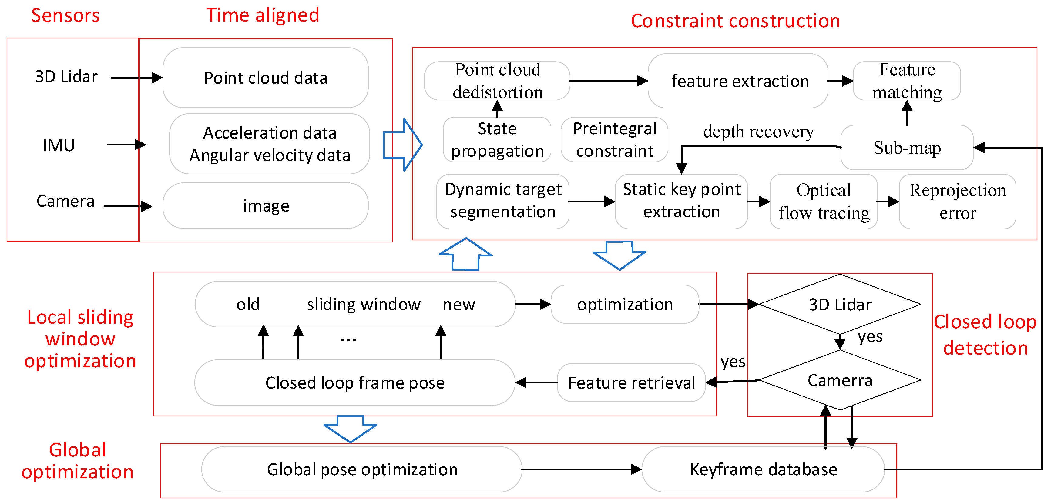
The LVI fusion framework designed in this paper consists of five parts as shown in Figure 1. Each module is described in detail below.
- (1)
- Time alignment. Regardless of systems triggered by external clocks (such as GNSS), each sensor is collected at a different start time stamp, and different sensors have different data acquisition frequencies. State fusion estimation requires aligning data with different timestamps to the same time node. LVI-fusion takes the camera time stamp as the benchmark, splits the lidar point cloud data according to the camera time stamp, and merges the point cloud data between image frames into one frame point cloud. IMU data is interpolated according to the time stamp of the camera to obtain IMU data aligned with the camera time stamp. Through the above operations, the lidar data, IMU data and camera data can be time-stamped aligned.
- (2)
- Data preprocessing. The state propagation of IMU data between adjacent image frames is carried out, and the point cloud data between two image frames is dedistorted according to the state prediction results, and the point cloud is unified to the end time of the point cloud of the frame. The YOLOv7 dynamic target recognition algorithm [47] is used to segment the dynamic target of the image, eliminate the influence of the dynamic target, obtain the static target image, construct the image pyramid of the deleted dynamic target image, extract the Harris key points from each layer of the image, and use the quadtree to homogenize the feature points to obtain uniformly distributed feature points. The tracked feature points are added to the image queue.
- (3)
- Constraint construction. The IMU data between adjacent image key frames are pre-integrated, the pre-integral increment of adjacent image key frames is obtained, and the Jacobian matrix and covariance of the pre-integral error matrix are constructed. The local point cloud map near the current key frame is used to assign depth to the image feature points, and the image feature points with depth are obtained. The reprojection error constraints are constructed according to the 3D coordinates of the feature points and the image frames tracked to their coordinates. Due to the high frequency of the camera, the field of view Angle of the lidar data with the camera time is less than half of the original, and the key frame is selected according to the pose result obtained by the VIO odometer. When it is a key frame, the lidar data of the current frame and the lidar data of the previous two frames are combined into one frame point cloud data. Line features and surface features are extracted from key frame point cloud data and matched with a local map to construct pose constraint based on lidar. According to IMU pre-integral constraints, visual reprojection constraints and lidar matching constraints, the nonlinear optimization objective function can be constructed, and the real-time pose calculation can be performed by using the sliding window optimization method, and the optimization results are fed back to the visual inertial odometer.
- (4)
- Closed loop detection. The closed-loop detection algorithm based on 3D lidar, and the visual-based bag of words model were used for closed-loop detection. When the constraints of both methods are met, the closed-loop constraints between visual and lidar are added to the global optimization.
- (5)
- Global optimization. Opens a separate thread for global optimization of keyframe-based pose.
3.1. Symbolic Description
, , , and represent the world coordinate system, IMU coordinate system, lidar coordinate system, and visual coordinate system, respectively. Define the body coordinate system to coincide with the IMU coordinate system. The variables represents all the variables in the sliding window. includes the state variables of keyframes within the sliding window, as well as the inverse depth of all feature points within the sliding window. represents the number of keyframes within the sliding window, and represents the number of key points. includes the position , velocity , attitude , acceleration bias , and angular velocity bias . and depict the rotation and shift of the body coordinate system to the world coordinate systemwhen the k-th image is taken, where is a quaternion. depicts the velocity of the body coordinate system to the world coordinate system when the k-th image is taken. . , , and are all three-dimensional vectors.
3.2. Time Aligned
There are two kinds of timestamps in ROS, one is the ROS system time stamp (ROS time), and the other is the time stamp of external hardware devices (such as cameras, lidar, etc.), also known as hardware time. The ROS timestamp is a floating-point number, measured in seconds, calculated from 00:00:00 UTC on 1 January 1970. The ROS timestamp is globally unique in the entire ROS system, that is, when nodes in the ROS system need to synchronize time, the ROS timestamp can be used as a standard, and each node can synchronize based on it. The hardware timestamp is provided by an external device and can be either a relative timestamp (the time difference between the device startup time or a fixed point in time) or an absolute timestamp (the time relative to a fixed point in time). Since the external device and the ROS system are different systems, their clocks may differ, so timestamp conversion is required to convert hardware timestamps to ROS timestamps, or ROS timestamps to hardware timestamps for operations such as time synchronization and data fusion. In this paper, we consider a system where lidar and camera are not triggered by an external clock (such as GNSS). In order to ensure the consistency of the time system, we assign time information to different sensor data according to the built-in time system of the robot operating system. The individual timestamp of the points can be obtained from the sensor’s driver. If the timestamp for a point is not available, it also can be calculated by orientation difference. After the time reference of the lidar point cloud, the camera, and IMU are aligned to the ROS time system, the time alignment operation can be performed. Since the startup time and frequency of different sensors are different, this paper takes the frequency of the camera as the benchmark. The lidar data is split and merged, and the point cloud located between the time stamps is repackaged into a frame of point cloud data according to the time stamps between the adjacent images, as shown in Figure 2. Image acquisition can be considered instantaneous, and the data of a frame of lidar point cloud is continuous. In this paper, a frame of lidar point cloud data is dedistorted to the last moment of the frame. As shown in Figure 3. For specific operations, refer to FAST-LIO2, and then it can be considered that the frame of lidar point cloud data is acquired synchronously with the camera.
The IMU and camera time stamps are synchronized by timestamp interpolation, and the IMU data before and after the camera time stamps are interpolated to obtain the IMU data corresponding to the image time stamps, as can be seen from Figure 4.
The K-frame acquisition time of the camera is . Due to the misalignment of time stamps, there is no IMU data at this time. The measured values of and before and after this time correspond to and respectively. The IMU data corresponding to can be interpolated according to the Formula (2) to realize the alignment of time stamps. Similarly, the measured value at time can be calculated according to Formula (3). Through the above processing, we do not need external timing equipment to complete the timestamp, which greatly increases the scene applicability of the system itself and provides a data basis for multi-sensor fusion based on graph optimization.
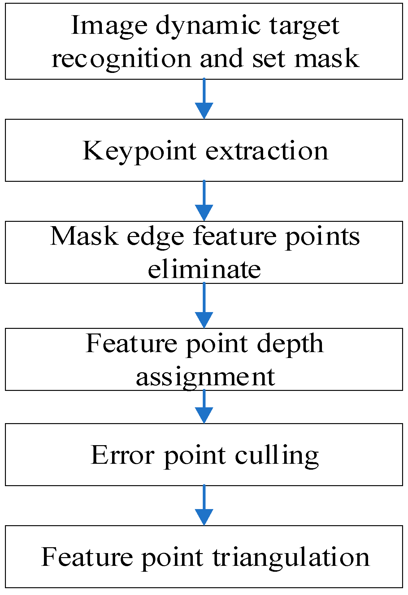
3.3. Key Point Depth Association
Robust key point depth recovery is very important for positioning accuracy and robustness. The key point depth reply process of this paper is shown in Figure 5. Firstly, dynamic target segmentation is carried out on the image, and key points are extracted from the static target image. Secondly, the key point of the mask region boundary is eliminated to eliminate the error key point caused by the mask. Then, the local point cloud map is used to assign the depth value to the static key points, and the key points that are wrong in terms of depth recovery are checked, and the key points without depth are restored by triangulation.
3.3.1. Image Target Detection
In recent years, real-time target detection algorithms have been developed rapidly. For example, MCUNet [48] and NanoDet [49] worked to improve model inference speed on low-power edge CPU chips. The Yolox [50] algorithm focuses on improving the speed of model inference on various GPU devices. At present, the development of real-time object detection algorithms focuses on the design of the efficient backbone network modules of models. For real-time object detection algorithms used on cpus, backbone network design is mainly based on MobileNet [51], ShuffleNet [52] or GhostNet [53]. On the other hand, on the GPU, most of the mainstream real-time target detection algorithms use ResNet [54] or DLA [55], and then use the gradient strategy in CSPNet [56] to further optimize the module. In addition to the design of the model backbone network, the YOLOv7 algorithm also pays special attention to the optimization of the model training process. These modules and methods can enhance the training effect and improve the accuracy of target detection, but do not increase the inference cost. The YOLOv7 backbone network is mainly composed of extended efficient layer aggregation networks (E-ELAN) [55], and features of three scales are used to detect output targets, as shown in Figure 6. The YOLOv7 algorithm can achieve a good detection effect while maintaining the detection speed. Therefore, this paper selects the YOLOv7 algorithm to complete image-based dynamic target detection.
Since YOLOv7 can detect a wide range of target categories, as shown in Figure 7b, in order to prevent static targets from being eliminated, this paper mainly identifies dynamic targets such as “people”, “bicycles”, “motorcycles” and “cars” according to realistic dynamic scenes, as shown in Figure 7c. In addition, in order to facilitate subsequent feature point extraction, the mask is set to pure white, as shown in Figure 7d.
Figure 8a shows the key points extraction results of images with deleted dynamic targets. Through Figure 8a, it is found that some key points have also been extracted on the contour of the dynamic target mask, which needs to be removed. Identify dynamic target edge feature points with a pixel value of 255 for surrounding pixels with a radius of 3 of key points and remove them. The elimination results are shown in Figure 8b. It can be found that the feature points on the edge of the dynamic feature are well eliminated and the key points under the static target image are obtained.
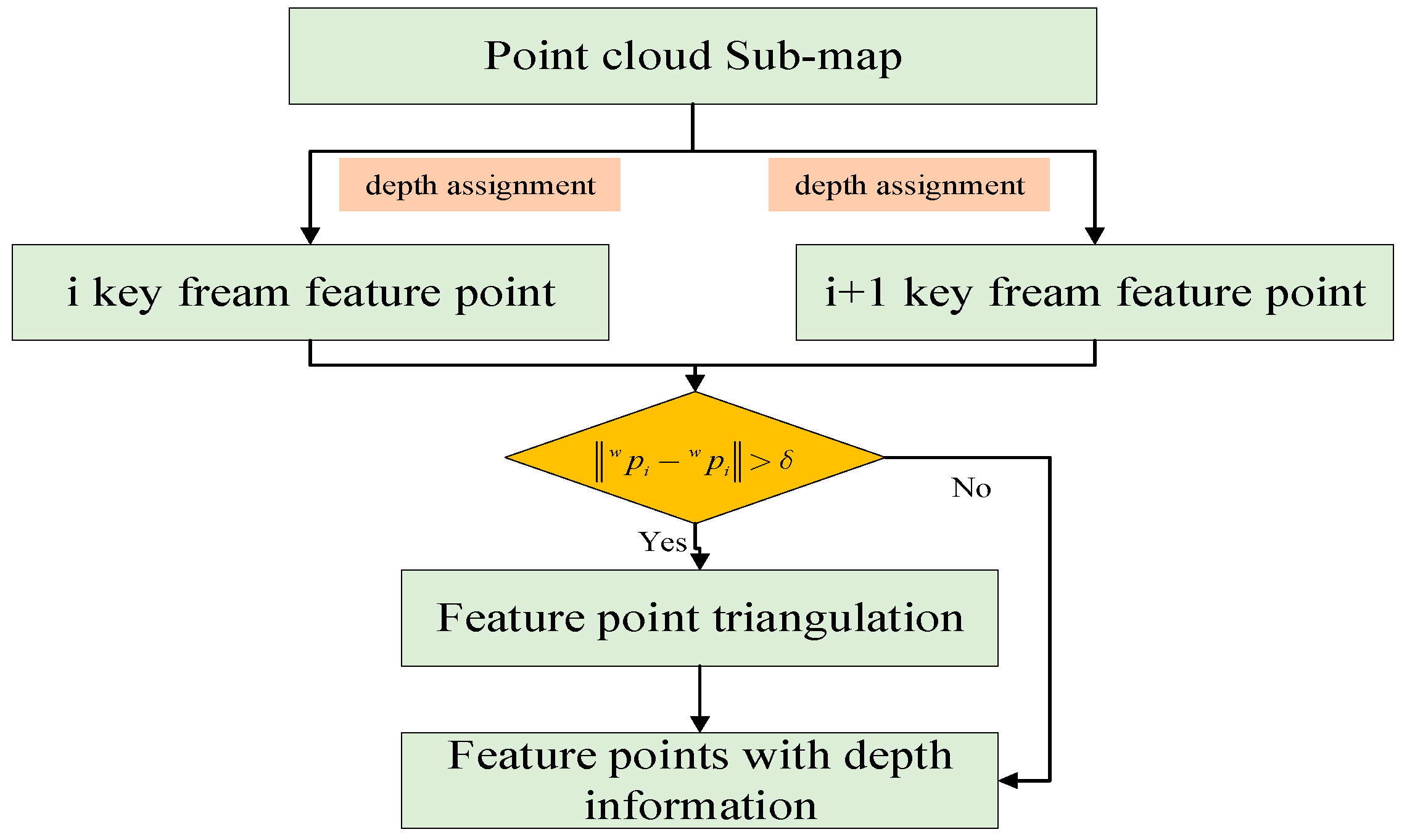
3.3.2. Key Point Depth Recovery
The sub-map is used to assign depth to each image key frame static key point. The feature points of the image are used to search for the three nearest-neighbor lidar points; the lidar points are fitted to the plane, and the distance between the feature points and the plane is calculated for depth assignment. When point is in the same plane as the surrounding lidar point cloud, the following functional relationship is satisfied:
represents the coordinates of point p in the world coordinate system, and represent the conversion relationship between the camera coordinate system and the world coordinate system under different field angles, respectively. and represent plane normal vectors fitted by lidar point clouds at different viewing angles, respectively. and represent the normalized image plane coordinates of the same key point under different viewing angles, respectively, which can be calculated according to pixel coordinates and camera parameters.
Due to the complexity of the real environment, and the feature points are basically the positions where the image gradient changes greatly, such positions are often not in the same plane with the three nearest lidar point clouds, resulting in wrong depth estimation. The relationship of formula 6 is no longer satisfied, as can be seen from Figure 9. Therefore, we can use this feature to test the correctness of the correlation between feature points and depth values. When the modulus length of the coordinate difference between and is less than a certain threshold, it is considered that the correlation of the depth value is correct; otherwise, the correlation of depth value of the feature point is cancelled, and the coordinate of the triangle point is restored based on visual triangulation; the process is shown in Figure 10.
3.4. Constraint Construction
3.4.1. Pre-Integration Factor
The acceleration model of IMU is shown in Formula (7), and the angular velocity model of IMU is shown in Formula (8).
and represent the raw measurements of the IMU sensor. The accelerometer noises and are assumed to obey white Gaussian noise, ,. represents rotation from the world coordinate system to the carrier coordinate system. represents the gravity vector in the world coordinate system, whose magnitude direction is known. The accelerometer bias and gyroscope bias follow random walks, as shown in Formulas (9) and (10).
There are multiple IMU data between the two image keyframes and . According to the dynamic equation of IMU, its integral form in continuous time is as follows:
where
, and represent the pose, velocity, and rotation angle corresponding to the pre-integral, respectively. The formula shows that the three quantities , and have no relationship with the state of . For two adjacent IMU observation data and , whose time interval is , Formula (11) can be written in a discretized form as Formula (13).
According to the equation of state and observation equation, the error equation of IMU can be obtained as Formula (14).
According to Formula (14), the variation formula of the covariance equation corresponding to the error equation over time can be derived by using the error propagation theorem, and the specific derivation form is referred to [57].
3.4.2. Vision Factor
The visual part is shown in Figure 11. Thanks to the lidar sensor, ranging information from lidar point clouds can be used to provide depth information for visual features, and with depth information, it is easy to obtain 3D (three-dimensional) coordinates of key points. In addition, the threshold is used to judge and screen out the key points of the wrong depth information. The method of triangulation within the sliding window is used to recover the 3D coordinates of visual key points with incorrect depth information. The above process ensures that the 3D coordinates of the visual key points are more robust. Reprojection error constraints can be constructed in the sliding window to constrain the pose. In addition, the coordinates of triangulated key points are optimized to ensure the robustness of the coordinates of the triangulated feature points. The construction process of the error constraint for the reprojection error is described below.
For the convenience of description, this study uses the pinhole camera model for modeling. The image observation value of the feature point in the i-th frame is (, ), and the point is projected to the -th frame based on the result of the IMU status prediction. The coordinate of the feature point in j-th frame can be calculated by Equation (15). The coordinates of feature point in j-th (, ) can be traced according to optical flow. According to the predicted feature point coordinates and the feature point coordinates of optical flow tracking, the reprojection error equation can be constructed, as shown in Equation (16). represents the inverse of the camera internal parameter matrix. Formula (17) is constructed by summing the square of all visual observation reprojection errors. represents the feature points observed at least twice in the sliding window. The maximum likelihood estimation of state variables can be obtained by the nonlinear solution of Equation (17) using the L-M method.
3.4.3. Lidar Factor
For time-stamped alignment with the vision sensor, the lidar data is divided and merged and the horizontal field of view angle of the repackaged point cloud data becomes one-third of the original when the frequency of the vision sensor is three times the frequency of the lidar sensor. Therefore, it is also difficult to match between frames based on the point cloud. It is necessary to build a local map to match the point cloud with the current frame. Therefore, this scheme needs to be stationary for a period of time, so that the lidar can fully scan and build a local map. When new time-aligned lidar data are received, we project the point cloud to the point cloud end time as FAST-LIO do. Surface features and line features are extracted from each frame of lidar and local point cloud map, and then matching constraints based on features are constructed. In order to maintain more efficient computing speed, ikd-Tree [35] is used for local map management and the nearest neighbor search of feature points. The construction process of feature extraction and lidar constraint is followed as LIO-SAM. Essentially, it minimizes the distance from the point to the line and the distance from the point to the surface, as shown in Formula (18).
represents the distance from the i-th line feature point to the line feature, represents the distance from the j-th plane feature point of to the corresponding plane. and represent the total number of line and surface features, respectively.
3.5. Local Sliding Window Optimization
The constraint factors constructed by different sensors all have common constraint variables, and the different constraint factors are combined, as shown in Formula (19). The first term in Equation (19) represents the marginalized prior information. The Levenberg–Marquardt method is adopted in this paper to optimize the solution of the constraint equation. The size of the window can be adjusted according to the performance of the computer.
3.6. Loopback Detection
This paper is based on the Scan Context (SC) [29] algorithm of 3D lidar for loop closure detection. In order to ensure that the lidar key frame can maintain a 360° field of view, the key frame is combined with the previous two frames of lidar data to form a frame of point cloud data and projected to the end of the key frame point cloud. Scan Context is calculated for each key frame and SC descriptors of different keyframes are matched to find point clouds in historical keyframes that are similar to current keyframes, so as to find loopback frames. It searches loopback frames by the similarity between the point clouds of individual keyframes, so it is not affected by geometric distance, and the loopback detection function can be completed even in large scenes. On this basis, the closed-loop detection of the visual word bag model is added. When the loopback detection of the above two methods is met at the same time, it is judged as a candidate frame. The sub-map is constructed with candidate frames for point cloud matching with the current frame. According to the matching situation, it is further determined whether it is a loop frame. When there is closed-loop detection, visual-based loop constraint and lidar loop constraint is added to the state estimation equation to minimize the cumulative error.
4. Experimental Setup and Evaluation
4.1. M2DGR Dataset
This paper uses the M2DGR dataset collected by Shanghai Jiao Tong University. M2DGR is the SLAM dataset collected by the ground robot navigation, which includes the look around RGB camera, infrared camera, event camera, 32-line lidar, IMU and original GNSS information, as shown in Figure 12. The dataset covers challenging scenes both indoor and outdoor, day and night, as shown in Figure 13. This paper selects 6 datasets from M2DGR for testing in different challenging scenarios and Table 4 summarizes the characteristics of different datasets.
4.1.1. Mapping Effect
All experiments in this paper were conducted in the Intel i7-107500H CPU test environment with 24 gb RAM. In this paper, the proposed algorithm LVI-fusion is used to test the mapping and positioning accuracy analysis. As shown in Figure 14, all scenes can establish accurate 3D point cloud maps. Next, we will further analyze the positioning track accuracy.
4.1.2. Precision Analysis
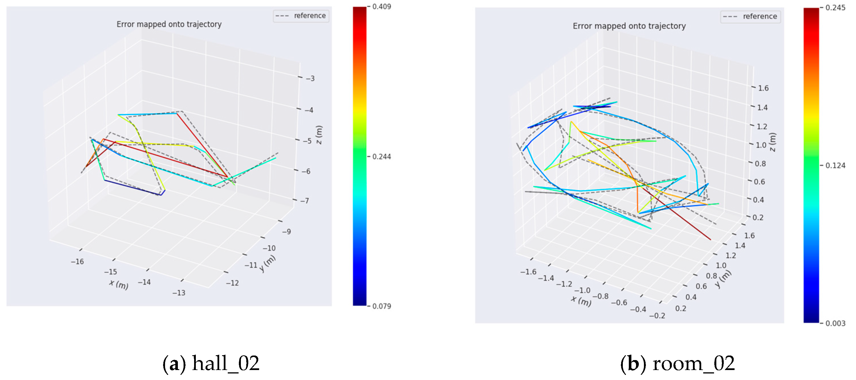
To show the positioning performance of LVI-fusion proposed in this paper, It can be seen intuitively from Figure 15 that there is no big deviation between LVI-fusion’s positioning trajectory and the truth trajectory, and the trajectory shape is basically the same. The bar on the right of Figure 15 represents the error range and the unit is meters.
In order to further analyze the positioning performance of the LVI-fusion proposed in this paper, this paper uses the RMSE (Root Mean Square Error) index to calculate the positioning accuracy of the LVI-fusion. In addition, in order to better demonstrate the competitiveness of the algorithm proposed in this paper, this paper uses the current outstanding and representative SLAM schemes including VINS-Mono, A-LOAM, LIO-SAM, and LVI-SAM to test the above 6 scenarios, respectively. Based on the above 10 scenarios, the RMSE indicators of different SLAM schemes are shown in Table 5. The RMSE calculation formula of the estimated trajectory based on different SLAM schemes is as follows:
where and respectively represent the estimated pose and truth pose at time i, respectively, where . Table 5 and Table 6 show the positioning accuracy of different SLAM schemes. Table 4 shows the odometer accuracy of different SLAM schemes without Loop closure detection, and Table 6 contains the positioning accuracy after loopback detection. Among them, A-LOAM does not have the loopback closure detection module, so this paper only tests the accuracy of the front-end odometer for these two SLAM schemes. It can be found from Table 5, that the positioning accuracy of the lidar-based positioning scheme is generally better than that of the VINS-Mono scheme based on visual inertia fusion. Among them, the positioning results of the proposed algorithm in this paper are generally better than the A-LOAM, VINS-Mono, and LIO-SAM schemes except for individual scenarios, showing the advantages of multi-source sensor fusion. Through the positioning accuracy in different scenarios, it is found that the LVI-fusion can achieve better positioning accuracy than LVI-SAM. This is because the coupling degree of the proposed algorithm is higher, and all variables are optimized and solved at the same time. As can be seen from Table 5, the accuracy of LVI-fusion proposed in this paper has a significant advantage compared with the existing representative SLAM scheme, and the accuracy is increased by more than 20% compared with the LVI-SAM scheme.
4.2. Low-Dynamic Environment
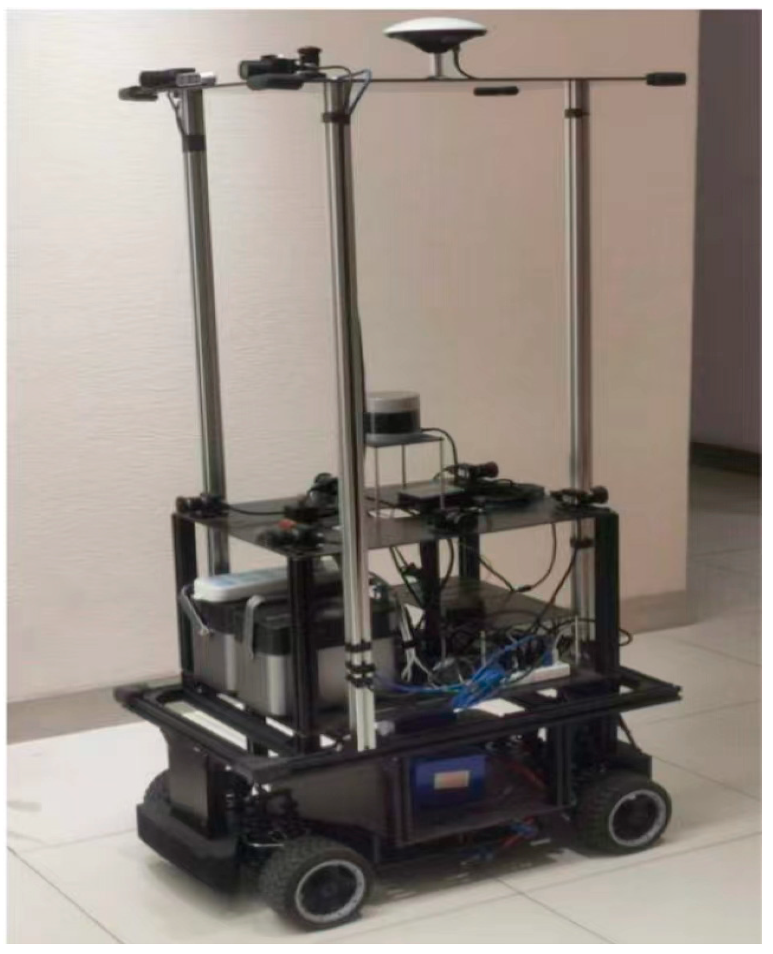
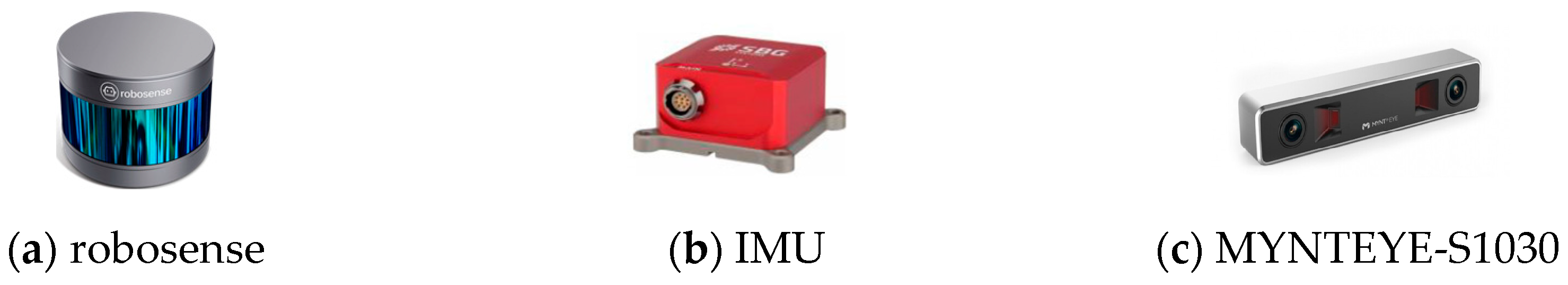
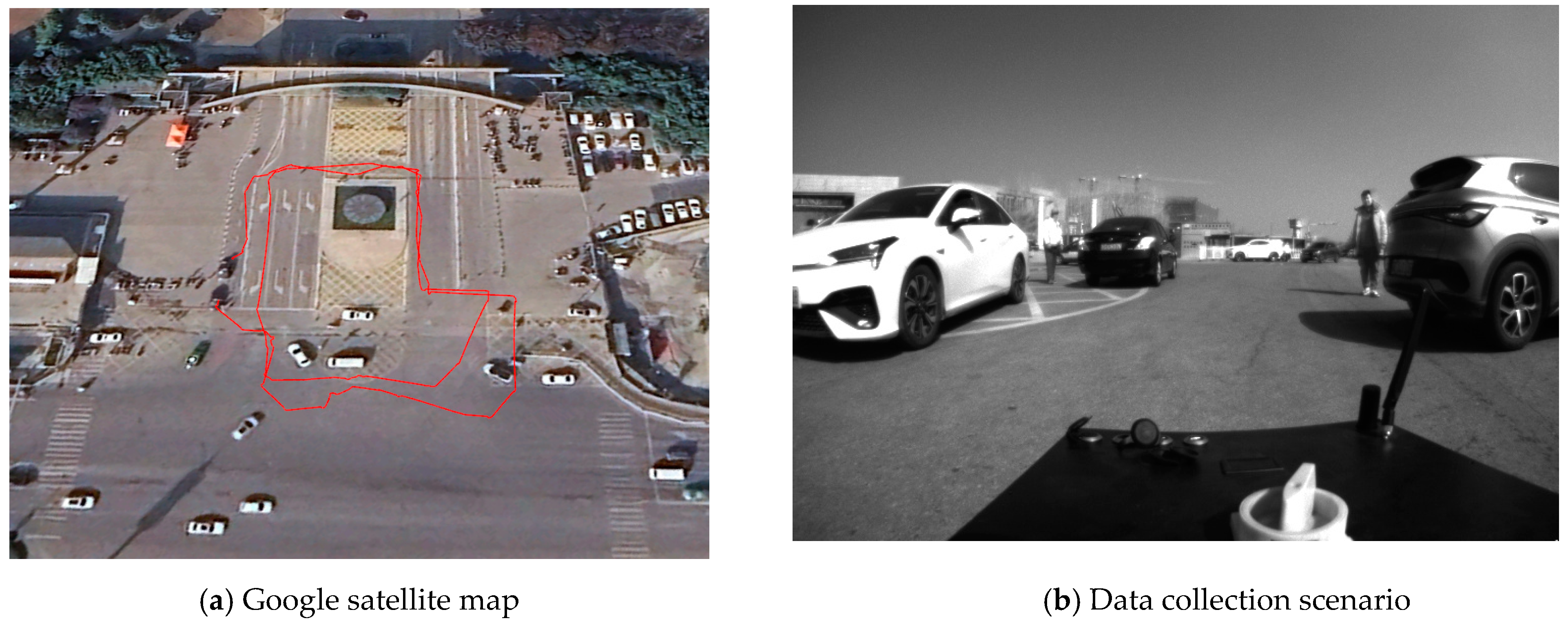
In this paper, data acquisition is carried out based on the tracked robot, which is equipped with a camera, IMU, multi-line lidar (Robosense 16), and RTK (real-time kinematic) module for obtaining the truth value [58], as shown in Figure 16. The parameter indicators of Lidar and IMU are shown in Table 7 and Table 8. The left eye of the MYNT EYE camera standard version is used as the image acquisition device, with an acquisition frequency of 25 Hz and a resolution of 752 × 480. Since the IMU is built into the tracked robot, it cannot be seen in Figure 16. We selected two representative scenes on the campus of China University of Mining and Technology, namely the square scene, the road scene, as shown in Figure 17, where the red trajectory is the positioning trajectory based on RTK.
4.2.1. Mapping Effect
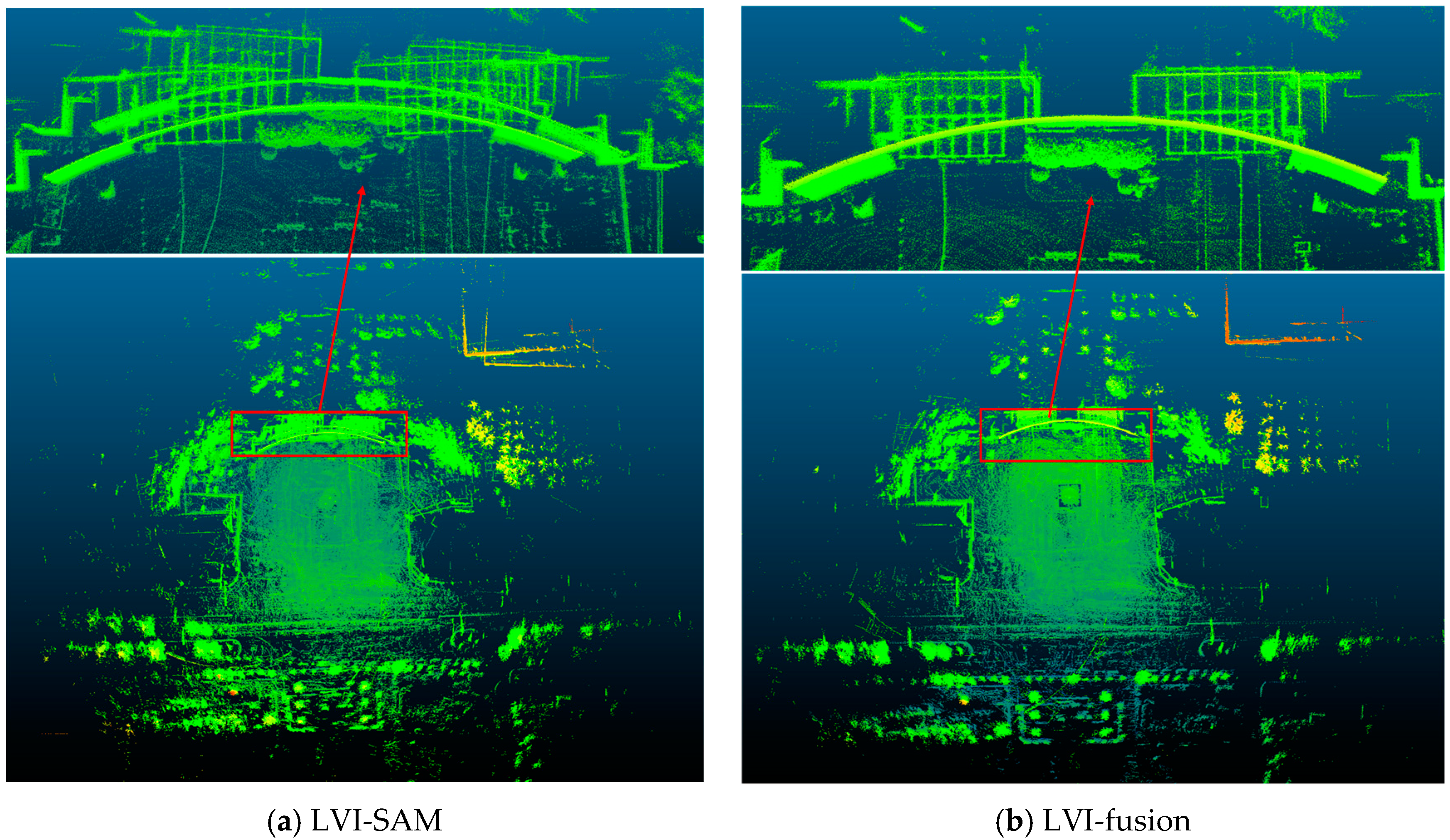
LVI-SAM is a multi- sensor fusion SLAM representative scheme based on graph optimization. In this paper, mapping experiments based on LVI-fusion and LVI-SAM are carried out based on the above three data, as shown in Figure 18 and Figure 19. It can be seen from Figure 18 and Figure 19 that LVI-fusion’s drawing effect is clearer and more accurate.
4.2.2. Precision Analysis
In this paper, the EVO tool is used to draw the trajectory error graph of LVI-fusion, as shown in Figure 20. Table 9 shows the RMSE of LIO-SAM, LVI-SAM and LVI-fusion. It can be seen that the scheme proposed in this paper has the best precision and is more stable. In low-dynamic scenes, it was found that LVI-fusion has the highest accuracy and LIO-SAM has the lowest accuracy, and the multiple sensor fusion has more positioning advantages. Due to the higher coupling degree of LVI-fusion, it can achieve better positioning accuracy compared to LVI-SAM.
4.3. High-Dynamic Environment
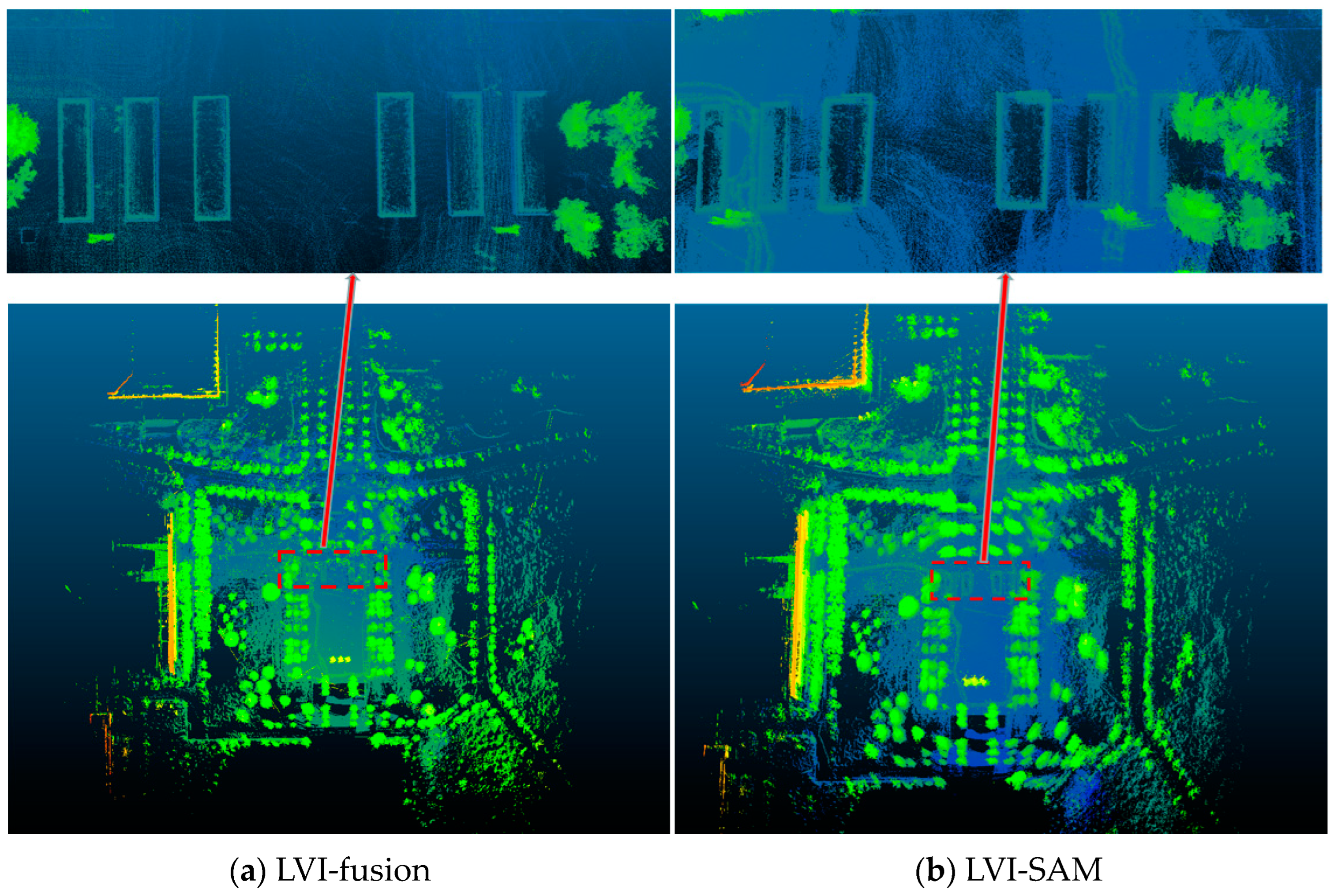
In order to verify the robustness of LVI-fusion in a dynamic environment, this paper selects the East gate of China University of Mining and Technology, a scene with abundant dynamic targets, as shown in Figure 21. The red trajectory in Figure 21a is the motion trajectory collected by the RTK positioning module. Figure 21b shows part of the data acquisition scenario. As can be seen from Figure 21b, the East gate of China University of Mining and Technology contains a large number of people, bicycles, electric vehicles, and taxis and other dynamic targets around the mobile measurement platform. Figure 22a shows the results of dynamic target segmentation based on the YOLOv7 dynamic target detection algorithm. Figure 22b shows the effect of the static key point extraction.
LIO-SAM and LVI-fusion are representatives of multi-source fusion SLAM schemes based on optimization. Figure 23 shows the positioning trajectory diagram of LIO-SAM, LVI-SAM and LVI-fusion proposed in this paper. It can be seen that LVI-SAM has the worst positioning effect in a dynamic environment. Due to the presence of a large number of dynamic targets in the environment, incorrect point cloud information assigns values to visual dynamic key points, further leading to incorrect matching of visual key points. Therefore, the combination of the two is not as effective in positioning in high-dynamic environments as the LIO-SAM scheme. Due to the removal of dynamic key points and the use of only static key points for visual constraints, as well as the use of depth information for judgment, LVI-fusion removes key points with incorrect assignment, resulting in better localization performance compared to LVI-SAM and LIO-SAM. From Table 10, it can be seen that LVI-fusion has the highest positioning accuracy, with a 26% improvement compared to LIO-SAM and a 40% improvement compared to LVI-SAM. Figure 24 shows the mapping results of LVI-SAM and LVI-fusion. It can be seen that LVI-fusion has higher mapping quality, and no significant point cloud overlap appears.
5. Conclusions
This article proposes a robust SLAM scheme LVI-fusion for lidar/vision/IMU fusion. This scheme proposes a sensor soft synchronization time alignment method and utilizes lidar cloud depth assignment and triangulation to achieve a maximum number of image key point depth recovery. In addition, this scheme utilizes the YOLOV7 object recognition algorithm to eliminate the erroneous effects caused by matching key points in dynamic environments, achieving robust multi-source fusion localization and mapping. The positioning accuracy on the M2DGR dataset indicates that LVI-fusion can achieve better positioning accuracy compared to the current representative SLAM scheme. In addition, data collection is carried out in low-dynamic and high-dynamic environments through the built mobile measurement platform. Compared with the LVI-SAM scheme, LVI-fusion improves positioning accuracy by about 20% in low-dynamic scenes and by about 40% in high-dynamic scenes. The above results indicate that the LVI-fusion proposed in this article has better positioning accuracy in both low-dynamic and high-dynamic environments. And in dynamic environments, LVI-fusion has better robustness.
Although the LVI-fusion proposed in this paper can be robustly positioned and mapping, offline calibration is needed to transplant the algorithm to different hardware platforms, which brings great inconvenience to cross-platform applications. Therefore, it is an urgent problem to realize the high-precision and robust online calibration of external parameters between each sensor based on LVI-fusion.
Author Contributions
Conceptualization, Z.L. (Zhenbin Liu) and Z.L. (Zengke Li); methodology, Z.L. (Zhenbin Liu) and Z.L. (Zengke Li); software, Z.L. (Zhenbin Liu), A.L., K.S., Q.G. and C.W.; validation, Z.L. (Zhenbin Liu), A.L., K.S., Q.G. and C.W.; formal analysis, Z.L. (Zhenbin Liu); investigation, Z.L. (Zhenbin Liu); resources, Z.L. (Zhenbin Liu); data curation, Z.L. (Zhenbin Liu), A.L. and C.W.; writing—original draft preparation, Z.L. (Zhenbin Liu); writing—review and editing, Z.L. (Zhenbin Liu); visualization, Z.L. (Zhenbin Liu); supervision, Z.L. (Zengke Li); project administration, Z.L. (Zengke Li); funding acquisition, Z.L. (Zengke Li). All authors have read and agreed to the published version of the manuscript.
Funding
This work was supported by the National Natural Science Foundation of China (No. 42274020), Science and Technology Planning Project of Jiangsu Province (BE2023692) and National Natural Science Foundation of China (No. 41874006) (Corresponding author: Zengke Li).
Data Availability Statement
No new data were created or analyzed in this study. Data sharing is not applicable to this article.
Conflicts of Interest
The authors declare that they have no conflicts of interest.
References
- Cadena, C.; Carlone, L.; Carrillo, H.; Latif, Y.; Scaramuzza, D.; Neira, J.; Reid, I.; Leonard, J.J. Past, Present, and Future of Simultaneous Localization and Mapping: Toward the Robust-Perception Age. IEEE Trans. Robot. 2016, 32, 1309–1332. [Google Scholar] [CrossRef]
- Li, J.; Pei, L.; Zou, D. Attention-SLAM: A Visual Monocular SLAM Learning From Human Gaze. IEEE Sens. J. 2021, 21, 6408–6420. [Google Scholar] [CrossRef]
- Debeunne, C.; Vivet, D. A review of visual-Lidar fusion based simultaneous localization and mapping. Sensors 2020, 20, 2068. [Google Scholar] [CrossRef] [PubMed]
- Forster, C.; Carlone, L.; Dellaert, F. On-Manifold Preintegration for Real-Time Visual—Inertial Odometry. IEEE Trans. Robot. 2017, 33, 1–21. [Google Scholar] [CrossRef]
- Tao, Y.; He, Y.; Ma, X. SLAM Method Based on Multi-Sensor Information Fusion. In Proceedings of the 2021 International Conference on Computer Network, Electronic and Automation (ICCNEA), Xi’an, China, 24–26 September 2021; pp. 289–293. [Google Scholar] [CrossRef]
- Yu, H.; Wang, Q.; Yan, C.; Feng, Y.; Sun, Y.; Li, L. DLD-SLAM: RGB-D Visual Simultaneous Localisation and Mapping in Indoor Dynamic Environments Based on Deep Learning. Remote Sens. 2024, 16, 246. [Google Scholar] [CrossRef]
- Huletski, A.; Kartashov, D.; Krinkin, K. Evaluation of the modern visual SLAM methods. In Proceedings of the 2015 Artificial Intelligence and Natural Language and Information Extraction, Social Media and Web Search FRUCT Conference (AINL-ISMW FRUCT), St. Petersburg, Russia, 9–14 November 2015; pp. 19–25. [Google Scholar] [CrossRef]
- Shan, T.; Englot, B.; Ratti, C. LVI-SAM: Tightly-Coupled Lidar-Visual-Inertial Odometry via Smoothing and Mapping. In Proceedings of the 2021 IEEE International Conference on Robotics and Automation (ICRA), Xi’an, China, 30 May 2021–5 June 2021; pp. 5692–5698. [Google Scholar] [CrossRef]
- Yin, J.; Li, A.; Li, T. M2DGR: A Multi-Sensor and Multi-Scenario SLAM Dataset for Ground Robots. IEEE Robot. Auto Let. 2022, 7, 2266–2273. [Google Scholar] [CrossRef]
- Chghaf, M.; Rodriguez, S.; Ouardi, A.E. Camera, LiDAR and Multi-modal SLAM Systems for Autonomous Ground Vehicles: A Survey. J. Intell. Robot. Syst. 2022, 105, 2. [Google Scholar] [CrossRef]
- Davison, A.J.; Reid, I.D.; Molton, N.D. MonoSLAM: Real-Time Single Camera SLAM. IEEE Trans. Pattern Anal. Mach. Intell. 2007, 29, 1052–1067. [Google Scholar] [CrossRef]
- Klein, G.; Murray, D. Parallel Tracking and Mapping for Small AR Workspaces. In Proceedings of the 2007 6th IEEE and ACM International Symposium on Mixed and Augmented Reality, Nara, Japan, 13–16 November 2007; pp. 225–234. [Google Scholar] [CrossRef]
- Mur-Artal, R.; Montiel, J.M. ORB-SLAM: A Versatile and Accurate Monocular SLAM System. IEEE Trans. Robot. 2017, 31, 1147–1163. [Google Scholar] [CrossRef]
- Rublee, E.; Rabaud, V.; Konolige, K. ORB: An efficient alternative to SIFT or SURF. In Proceedings of the IEEE International Conference on Computer Vision, ICCV 2011, Barcelona, Spain, 6–13 November 2011. [Google Scholar] [CrossRef]
- Mur-Artal, R.; Tardós, J.D. ORB-SLAM2: An Open-Source SLAM System for Monocular, Stereo, and RGB-D Cameras. IEEE Trans. Robot. 2017, 33, 1255–1262. [Google Scholar] [CrossRef]
- Forster, C.; Pizzoli, M.; Scaramuzza, D. SVO: Fast semi-direct monocular visual odometry. In Proceedings of the 2014 IEEE International Conference on Robotics and Automation (ICRA), Hong Kong, China, 31 May–7 June 2014; pp. 15–22. [Google Scholar] [CrossRef]
- Engel, J.; Thomas, S.; Cremers, D. Lsd-Salm: Large-Scale Direct Monocular Salm. In Proceedings of the European Conference on Computer Vision, Cham, Switzerland, 6–12 September 2014; pp. 834–849. [Google Scholar] [CrossRef]
- Engel, J.; Koltun, V.; Cremers, D. Direct Sparse Odometry. IEEE Trans. Pattern Anal. Mach. Intell. 2018, 40, 611–625. [Google Scholar] [CrossRef] [PubMed]
- Mourikis, A.I.; Roumeliotis, S.I. A Multi-State Constraint Kalman Filter for Vision-aided Inertial Navigation. In Proceedings of the 2007 IEEE International Conference on Robotics and Automation, Rome, Italy, 10–14 April 2007; pp. 3565–3572. [Google Scholar] [CrossRef]
- Leutenegger, S.; Lynen, S.; Bosse, M. Keyframe-based visual–inertial odometry using nonlinear optimization. Int. J. Robot. Res. 2015, 34, 314–334. [Google Scholar] [CrossRef]
- Qin, T.; Li, P.; Shen, S.T. VINS-Mono: A Robust and Versatile Monocular Visual-Inertial State Estimator. IEEE Trans. Robot. 2018, 34, 1004–1020. [Google Scholar] [CrossRef]
- Qin, T.; Pan, J.; Cao, S. A general optimization-based framework for local odometry estimation with multiple sensors. arXiv 2019, arXiv:1901.03638. [Google Scholar] [CrossRef]
- Campos, C.; Elvira, R.; Rodríguez, J.J.G. Orb-slam3: An accurate open-source library for visual, visual–inertial, and multimap slam. IEEE Trans. Robot. 2021, 37, 1874–1890. [Google Scholar] [CrossRef]
- Hess, W.; Kohler, D.; Rapp, H. Real-time loop closure in 2D LIDAR SLAM. In Proceedings of the 2016 IEEE International Conference on Robotics and Automation (ICRA), Stockholm, Sweden, 16–21 May 2016; pp. 1271–1278. [Google Scholar] [CrossRef]
- Zhang, J.; Singh, S. LOAM: Lidar Odometry and Mapping in Real-time. Robot. Sci. Syst. 2014, 2, 1–9. [Google Scholar]
- Qin, T.; Cao, S. A-LOAM. 2018. Available online: https://github.com/HKUST-Aerial-Robotics/A-LOAM (accessed on 23 April 2024).
- Shan, T.; Englot, B. LeGO-LOAM: Lightweight and Ground-Optimized Lidar Odometry and Mapping on Variable Terrain. In Proceedings of the 2018 IEEE/RSJ International Conference on Intelligent Robots and Systems (IROS), Madrid, Spain, 1–5 October 2018; pp. 4758–4765. [Google Scholar] [CrossRef]
- Kimm, G. SC-LeGO-LOAM. 2020. Available online: https://gitee.com/zhankun3280/lslidar_c16_lego_loam (accessed on 23 April 2024).
- Kim, G.; Kim, A. Scan Context: Egocentric Spatial Descriptor for Place Recognition within 3D Point Cloud Map. In Proceedings of the 2018 IEEE/RSJ International Conference on Intelligent Robots and Systems (IROS), Madrid, Spain, 1–5 October 2018; pp. 4802–4809. [Google Scholar] [CrossRef]
- Zhao, S.; Fang, Z.; Li, H. A Robust Laser-Inertial Odometry and Mapping Method for Large-Scale Highway Environments. In Proceedings of the 2019 IEEE/RSJ International Conference on Intelligent Robots and Systems (IROS), Macau, China, 3–8 November 2019; pp. 1285–1292. [Google Scholar] [CrossRef]
- Ye, H.; Chen, Y.; Liu, M. Tightly Coupled 3D Lidar Inertial Odometry and Mapping. In Proceedings of the 2019 International Conference on Robotics and Automation (ICRA), Montreal, QC, Canada, 20–24 May 2019; pp. 3144–3150. [Google Scholar] [CrossRef]
- Shan, T.; Englot, B.; Meyers, D. LIO-SAM: Tightly-coupled Lidar Inertial Odometry via Smoothing and Mapping. In Proceedings of the 2020 IEEE/RSJ International Conference on Intelligent Robots and Systems (IROS), Las Vegas, NV, USA, 24 October 2020–24 January 2021; pp. 5135–5142. [Google Scholar] [CrossRef]
- Qin, C.; Ye, H.; Pranata, C.E. LINS: A Lidar-Inertial State Estimator for Robust and Efficient Navigation. In Proceedings of the 2020 IEEE International Conference on Robotics and Automation (ICRA), Paris, France, 31 May–31 August 2020; pp. 8899–8906. [Google Scholar] [CrossRef]
- Xu, W.; Zhang, F. FAST-LIO: A Fast, Robust Lidar-Inertial Odometry Package by Tightly-Coupled Iterated Kalman Filter. IEEE Robot. Autom. Let. 2020, 6, 3317–3324. [Google Scholar] [CrossRef]
- Xu, W.; Cai, Y.; He, D. FAST-LIO2: Fast Direct Lidar-Inertial Odometry. IEEE Trans. Robot. 2022, 38, 2053–2073. [Google Scholar] [CrossRef]
- Bai, C.; Xiao, T.; Chen, Y. Faster-LIO: Lightweight Tightly Coupled Lidar-Inertial Odometry Using Parallel Sparse Incremental Voxels. IEEE Robot. Autom. Let. 2022, 7, 4861–4868. [Google Scholar] [CrossRef]
- Graeter, J.; Wilczynski, A.; Lauer, M. LIMO: Lidar-Monocular Visual Odometry. In Proceedings of the 2018 IEEE/RSJ International Conference on Intelligent Robots and Systems (IROS), Madrid, Spain, 1–5 October 2018; pp. 7872–7879. [Google Scholar] [CrossRef]
- Zhang, J.; Singh, S. Visual-Lidar odometry and mapping: Low-drift, robust, and fast. In Proceedings of the 2015 IEEE International Conference on Robotics and Automation (ICRA), Seattle, WA, USA, 26–30 May 2015; pp. 2174–2181. [Google Scholar] [CrossRef]
- Geiger, A.; Lenz, P.; Stiller, C. Vision meets robotics: The kitti dataset. Int. J. Robot. Res. 2013, 32, 1231–1237. [Google Scholar]
- Shao, W.; Vijayarangan, S.; Li, C. Stereo Visual Inertial Lidar Simultaneous Localization and Mapping. In Proceedings of the 2019 IEEE/RSJ International Conference on Intelligent Robots and Systems (IROS), Macau, China, 3–8 November 2019; pp. 370–377. [Google Scholar] [CrossRef]
- Zuo, X.; Geneva, P.; Lee, W. LIC-Fusion: Lidar-Inertial-Camera Odometry. In Proceedings of the 2019 IEEE/RSJ International Conference on Intelligent Robots and Systems (IROS), Macau, China, 3–8 November 2019; pp. 5848–5854. [Google Scholar] [CrossRef]
- Zuo, X. LIC-Fusion 2.0: Lidar-Inertial-Camera Odometry with Sliding-Window Plane-Feature Tracking. In Proceedings of the 2020 IEEE/RSJ International Conference on Intelligent Robots and Systems (IROS), Las Vegas, NV, USA, 24 October 2020–24 January 2021; pp. 5112–5119. [Google Scholar] [CrossRef]
- Wisth, D.; Camurri, M.; Das, S. Unified Multi-Modal Landmark Tracking for Tightly Coupled Lidar-Visual-Inertial Odometry IEEE Robot. Autom. Let. 2021, 6, 1004–1011. [Google Scholar] [CrossRef]
- Lin, J.; Zheng, C.; Xu, W. R2 LIVE: A Robust, Real-Time, Lidar-Inertial-Visual Tightly-Coupled State Estimator and Mapping. IEEE Robot. Autom. Let. 2021, 6, 7469–7476. [Google Scholar] [CrossRef]
- Lin, J.; Zheng, C. R3LIVE: A Robust, Real-time, RGB-colored, Lidar-Inertial-Visual tightly-coupled state Estimation and mapping package. In Proceedings of the 2022 International Conference on Robotics and Automation (ICRA), Philadelphia, PA, USA, 23–27 May 2022; pp. 10672–10678. [Google Scholar] [CrossRef]
- Zheng, C. FAST-LIVO: Fast and Tightly-coupled Sparse-Direct Lidar-Inertial-Visual Odometry. In Proceedings of the 2022 IEEE/RSJ International Conference on Intelligent Robots and Systems (IROS), Kyoto, Japan, 23–27 October 2022. [Google Scholar] [CrossRef]
- Wang, C.Y.; Bochkovskiy, A.; Liao, H.Y.M. YOLOv7: Trainable bag-of-freebies sets new state-of-the-art for real-time object detectors. In Proceedings of the 2023 IEEE/CVF Conference on Computer Vision and Pattern Recognition (CVPR), Vancouver, BC, Canada, 17–24 June 2023. [Google Scholar] [CrossRef]
- Lin, J.; Chen, W.M.; Lin, Y.; Cohn, J.; Han, S. MCUNet: Tiny Deep Learning on IoT Devices. arXiv 2007, arXiv:2007.10319. [Google Scholar] [CrossRef]
- Lyu, R. Nanodet-Plus: Super Fast and High Accuracy Lightweight Anchor-Free Object Detection Model. 2021. Available online: https://github.com/RangiLyu/nanodet (accessed on 23 April 2024).
- Ge, Z.; Liu, S.; Wang, F. Yolox: Exceeding yolo series in 2021. arXiv 2021, arXiv:2107.08430. [Google Scholar] [CrossRef]
- Michele, A.; Colin, V.; Santika, D.D. Mobilenet convolutional neural networks and support vector machines for palmprint recognition. Procedia Comput. Sci. 2019, 157, 110–117. [Google Scholar] [CrossRef]
- Zhang, X.; Zhou, X.; Lin, M. Shufflenet: An extremely efficient convolutional neural network for mobile devices. In Proceedings of the IEEE Conference on Computer Vision and Pattern Recognition, Salt Lake City, UT, USA, 18–22 June 2018; pp. 6848–6856. [Google Scholar] [CrossRef]
- Han, K.; Wang, Y.; Tian, Q. Ghostnet: More features from cheap operations. In Proceedings of the IEEE/CVF Conference on Computer Vision and Pattern Recognition, Seattle, WA, USA, 13–19 June 2020; pp. 1580–1589. [Google Scholar] [CrossRef]
- Targ, S.; Almeida, D.; Lyman, K. Resnet in resnet: Generalizing residual architectures. arXiv 2016, arXiv:1603.08029. [Google Scholar] [CrossRef]
- Yu, F.; Wang, D.; Shelhamer, E. Deep layer aggregation. In Proceedings of the IEEE Conference on Computer Vision and Pattern Recognition, Salt Lake City, UT, USA, 18–23 June 2018; pp. 2403–2412. [Google Scholar] [CrossRef]
- Wang, C.Y.; Liao, H.Y.M.; Wu, Y.H. CSPNet: A new backbone that can enhance learning capability of CNN. In Proceedings of the IEEE/CVF Conference on Computer Vision and Pattern Recognition Workshops, Seattle, WA, USA, 14–19 June 2020; pp. 390–391. [Google Scholar] [CrossRef]
- Sol’a, J. Quaternion kinematics for the error-state Kalman filter. arXiv 2017, arXiv:1711.02508. [Google Scholar] [CrossRef]
- Teunissen, P.J.G.; Khodabandeh, A. Review and principles of PPP-RTK methods. J. Geod. 2015, 89, 217–240. [Google Scholar] [CrossRef]
Figure 1.
LVI-fusion framework based on visual, lidar and IMU fusion.

Figure 2.
Time aligned: split-and-merge; dotted lines refer to the camera timestamp, and solid lines refer to the lidar timestamp. Lidar point cloud data is split and merged based on the camera timestamp (Stars represents the timestamp corresponding to the data collected by the camera).
Figure 2.
Time aligned: split-and-merge; dotted lines refer to the camera timestamp, and solid lines refer to the lidar timestamp. Lidar point cloud data is split and merged based on the camera timestamp (Stars represents the timestamp corresponding to the data collected by the camera).

Figure 3.
Align the point cloud to the end of the frame.

Figure 4.
The IMU is aligned with the camera timestamp (Arrows correspond to the time of data collection).
Figure 4.
The IMU is aligned with the camera timestamp (Arrows correspond to the time of data collection).

Figure 5.
Key points depth recovery process.

Figure 6.
Network structure of YOLOV7 model.

Figure 7.
Schematic diagram of removing dynamic objects from YOLOv7. (a) Original image. (b) Original segmentation. (c) Specific dynamic target segmentation. (d) Dynamic target white mask.
Figure 7.
Schematic diagram of removing dynamic objects from YOLOv7. (a) Original image. (b) Original segmentation. (c) Specific dynamic target segmentation. (d) Dynamic target white mask.

Figure 8.
Static key points extraction results after tuning quadtree homogenization. (a) Quadtree equalization after removing dynamic targets. (b) Mask edge feature points are eliminated.
Figure 8.
Static key points extraction results after tuning quadtree homogenization. (a) Quadtree equalization after removing dynamic targets. (b) Mask edge feature points are eliminated.

Figure 9.
The projection relationship of the same key point under different keyframe perspectives.

Figure 10.
Process of determining the wrong depth assignment of feature points.

Figure 11.
Structure diagram of visual restraint.

Figure 12.
Sensor integration platform.

Figure 13.
M2DGR dataset partial scenarios.

Figure 14.
The mapping results of the mode 3 proposed in this paper.

Figure 15.
Track error of LVI-fusion proposed in this paper. Reference represents the truth value in the dataset, represented by a dotted line. The colored trajectory indicates the LVI-fusion running trajectory, and different colors indicate different degrees of error.
Figure 15.
Track error of LVI-fusion proposed in this paper. Reference represents the truth value in the dataset, represented by a dotted line. The colored trajectory indicates the LVI-fusion running trajectory, and different colors indicate different degrees of error.


Figure 16.
Mobile measurement platform based on tracked robot.


Figure 17.
Data acquisition environment satellite map.

Figure 18.
Comparison of map construction effect based on LVI-SAM and LVI-fusion in the road scene (the picture the arrow points to is a detailed enlarged photo of the box).
Figure 18.
Comparison of map construction effect based on LVI-SAM and LVI-fusion in the road scene (the picture the arrow points to is a detailed enlarged photo of the box).

Figure 19.
Comparison of map construction effect based on LVI-SAM and LVI-fusion in the square scene (the picture the arrow points to is a detailed enlarged photo of the box).
Figure 19.
Comparison of map construction effect based on LVI-SAM and LVI-fusion in the square scene (the picture the arrow points to is a detailed enlarged photo of the box).

Figure 20.
The colored trajectory indicates the LVI-fusion running trajectory, and different colors indicate different degrees of error.
Figure 20.
The colored trajectory indicates the LVI-fusion running trajectory, and different colors indicate different degrees of error.

Figure 21.
Data acquisition of the 3D lidar/Vision/IMU dynamic scene.

Figure 22.
Static feature point extraction (The green dots represent the extracted key points).

Figure 23.
Positioning track of LIO-SAM, LVI-SAM and LVI-fusion.

Figure 24.
Mapping effect of LVI-SAM and LVI-fusion.


Table 1.
Representational SLAM scheme based on visual and IMU.
| Scheme | Release Time | Sensor Form | Characteristic |
|---|---|---|---|
| MonoSLAM [11] | 2007 | a | EKF + Feature point method |
| PTAM [12] | 2007 | a | Feature point method |
| ORB-SLAM [13] | 2011 | a | ORB feature point method |
| ORB-SLAM2 [15] | 2015 | b | ORB feature + multiple mode cameras |
| SVO [16] | 2014 | a | Semi-direct method |
| LSD-SLAM [17] | 2014 | a | Direct method + semi-dense reconstruction |
| DSO [18] | 2020 | b | Direct method+ Sparse reconstruction |
| MSCKF [19] | 2020 | c | IESKF (iterative error state Kalman filter) |
| OKVIS [20] | 2020 | c | Key frame + graph optimization |
| VINS-mono [21] | 2017 | c | Optical flow + graph optimization |
| VINS-fusion [22] | 2019 | c | Optical flow + multimode |
| ORB-SLAM3 [23] | 2021 | c | ORB feature+ multimode |
a indicates support for monocular camera, b indicates support for multiple mode cameras, and c indicates support for visual integration with IMU.
Table 2.
Visual-inertial navigation system (VINS) scheme for visual inertial measurement unit (IMU) fusion.
Table 2.
Visual-inertial navigation system (VINS) scheme for visual inertial measurement unit (IMU) fusion.
| Scheme | Release Time | Sensor Form | Characteristic |
|---|---|---|---|
| LOAM [25] | 2014 | a | Milestone, based on feature matching |
| A-LOAM [26] | 2018 | a | Streamline LOAM code with optimization library |
| LeGO-LOAM [27] | 2018 | a | Ground point filtering, point cloud clustering |
| SC-LeGO-LOAM [28] | 2020 | a | Add loopback detection based on Scan Context |
| LIOM [30] | 2020 | b | CNN dynamic target elimination; ESKF filtering |
| LIO-Mapping [31] | 2019 | b | Graph optimization method |
| LIO-SAM [32] | 2020 | b | Factor graph optimization method |
| LINS [33] | 2020 | b | IESKF (iterative error state Kalman filter) |
| FAST-LIO [34] | 2020 | b | IEKF (Iterative Extended Kalman Filtering) |
| FAST-LIO2 [35] | 2021 | b | Incremental KD data structure (fast efficiency) |
| Faster-LIO [36] | 2022 | b | Use iVox data structure based on FAST-LIO2 to further improve efficiency |
a indicates support for 3D lidar, b indicates support for 3D lidar and IMU.
Table 3.
Representative slam scheme based on visual and lidar fusion.
| Scheme | Release Time | Sensor Form | Characteristic |
|---|---|---|---|
| LIMO [37] | 2018 | a | lidar-assisted visual recovery of feature point depth |
| V-LOAM [38] | 2018 | a | Match from high frequency to low frequency |
| VIL-SLAM [40] | 2019 | b | VIO assisted lidar positioning |
| LIC_Fusion [41] | 2019 | b | MSCKF filter (sensor online calibration) |
| LIC_Fusion2 [42] | 2020 | b | Sliding window filter |
| ULVIO [43] | 2021 | b | Factor Graph Optimization |
| R2live [44] | 2021 | b | ESKF filtering + factor graph optimization |
| R3live [45] | 2021 | b | Minimize the photometric error from frame to map |
| LVI-SAM [8] | 2021 | b | Factor Graph Optimization |
| FAST-LIVO [46] | 2022 | b | IESKF filtering |
a indicates support for 3D lidar and camera, b indicates support for 3D lidar, camera and IMU.
Table 4.
The characteristics of different datasets in M2DGR.
| Sequence Name | Duration (s) | Features |
|---|---|---|
| hall_02 | 128 | random walk, indoor, day |
| room_02 | 75 | room, bright, indoor, day |
| door_02 | 127 | outdoor to indoor, short-term, day |
| gate_03 | 283 | outdoor, day |
| walk_01 | 291 | back and forth, outdoor, day |
| street_05 | 469 | straight line, outdoor, night, |
Table 5.
Comparing the (rmse)/m results of VINS-Mono, A-LOAM, LIO-SAM, LVI-SAM and our method based on M2DGR datasets (without loop closure).
Table 5.
Comparing the (rmse)/m results of VINS-Mono, A-LOAM, LIO-SAM, LVI-SAM and our method based on M2DGR datasets (without loop closure).
| Approach | Hall_02 | Room_02 | Door_02 | Gate_03 | Walk_01 | Street_05 |
|---|---|---|---|---|---|---|
| VINS-Mono | fail | 0.462 | 1.653 | 5.838 | 9.976 | fail |
| A-LOAM | 0.208 | 0.121 | 0.168 | 0.246 | 3.303 | 0.657 |
| LIO-SAM | 0.399 | 0.125 | 0.124 | 0.111 | 0.891 | 0.407 |
| LVI-SAM | 0.279 | 0.123 | 0.186 | 0.113 | 0.885 | 0.394 |
| LVI-fusion | 0.214 | 0.103 | 0.117 | 0.104 | 0.627 | 0.371 |
Table 6.
Comparing the (rmse)/m results of VINS-Mono, A-LOAM, LIO-SAM, LVI-SAM and our method based on M2DGR datasets (with loop clousure).
Table 6.
Comparing the (rmse)/m results of VINS-Mono, A-LOAM, LIO-SAM, LVI-SAM and our method based on M2DGR datasets (with loop clousure).
| Approach | Hall_02 | Room_02 | Door_02 | Gate_03 | Walk_01 | Street_05 |
|---|---|---|---|---|---|---|
| VINS-Mono | fail | 0.311 | 1.522 | 5.838 | 9.976 | fail |
| LIO-SAM | 0.291 | 0.125 | 0.106 | 0.111 | 0.830 | 0.405 |
| LVI-SAM | 0.270 | 0.120 | 0.171 | 0.114 | 0.888 | 0.395 |
| LVI-fusion | 0.181 | 0.101 | 0.099 | 0.105 | 0.631 | 0.370 |
Table 7.
RS-LiDAR-16 parameters.
| Parameter | RS-LiDAR-16 | |
|---|---|---|
| Ranging range | 20 cm~150 m | |
| Distance measurement accuracy | ±2 cm | |
| Field of view angle | horizontal | 360° |
| Vertical | +15°~−15° | |
| Angle resolution | horizontal | 0.2° |
| Vertical | 2° | |
| Collect points per second | 28,800 | |
| scan period | 0.1 s | |
Table 8.
IMU parameters.
| Parameter | Index | |
|---|---|---|
| Accelerometer | Speed Random Walk () | 57 |
| Zero bias instability () | 14 | |
| gyroscope | angle random walk() | 0.18 |
| Zero bias instability () | 8 | |
| magnetometer | Noise (m Gauss) | 3 |
| Zero bias stability (m Gauss) | 1 |
Table 9.
Comparing the (rmse)/m results of LIO-SAM, LVI-SAM and LVI-fusion.
| Approach | Road Scene (m) | Square Scene (m) |
|---|---|---|
| LIO-SAM | 1.16 | 1.09 |
| LVI-SAM | 1.04 | 0.98 |
| LVI-fusion | 0.80 | 0.79 |
Table 10.
LIO-SAM, LVI-SAM, and LVI-fusion positioning accuracy.
| Representative SLAM Scheme | LIO-SAM | LVI-SAM | LVI-Fusion |
|---|---|---|---|
| RMSE(m) | 1.201 | 1.548 | 0.890 |
Disclaimer/Publisher’s Note: The statements, opinions and data contained in all publications are solely those of the individual author(s) and contributor(s) and not of MDPI and/or the editor(s). MDPI and/or the editor(s) disclaim responsibility for any injury to people or property resulting from any ideas, methods, instructions or products referred to in the content. |
© 2024 by the authors. Licensee MDPI, Basel, Switzerland. This article is an open access article distributed under the terms and conditions of the Creative Commons Attribution (CC BY) license (https://creativecommons.org/licenses/by/4.0/).
Share and Cite
MDPI and ACS Style
Liu, Z.; Li, Z.; Liu, A.; Shao, K.; Guo, Q.; Wang, C. LVI-Fusion: A Robust Lidar-Visual-Inertial SLAM Scheme. Remote Sens. 2024, 16, 1524. https://0-doi-org.brum.beds.ac.uk/10.3390/rs16091524
AMA Style
Liu Z, Li Z, Liu A, Shao K, Guo Q, Wang C. LVI-Fusion: A Robust Lidar-Visual-Inertial SLAM Scheme. Remote Sensing. 2024; 16(9):1524. https://0-doi-org.brum.beds.ac.uk/10.3390/rs16091524
Chicago/Turabian StyleLiu, Zhenbin, Zengke Li, Ao Liu, Kefan Shao, Qiang Guo, and Chuanhao Wang. 2024. "LVI-Fusion: A Robust Lidar-Visual-Inertial SLAM Scheme" Remote Sensing 16, no. 9: 1524. https://0-doi-org.brum.beds.ac.uk/10.3390/rs16091524
Note that from the first issue of 2016, this journal uses article numbers instead of page numbers. See further details here.