
EAD-Net: Efficiently Asymmetric Network for Semantic Labeling of High-Resolution Remote Sensing Images with Dynamic Routing Mechanism

Abstract
:1. Introduction
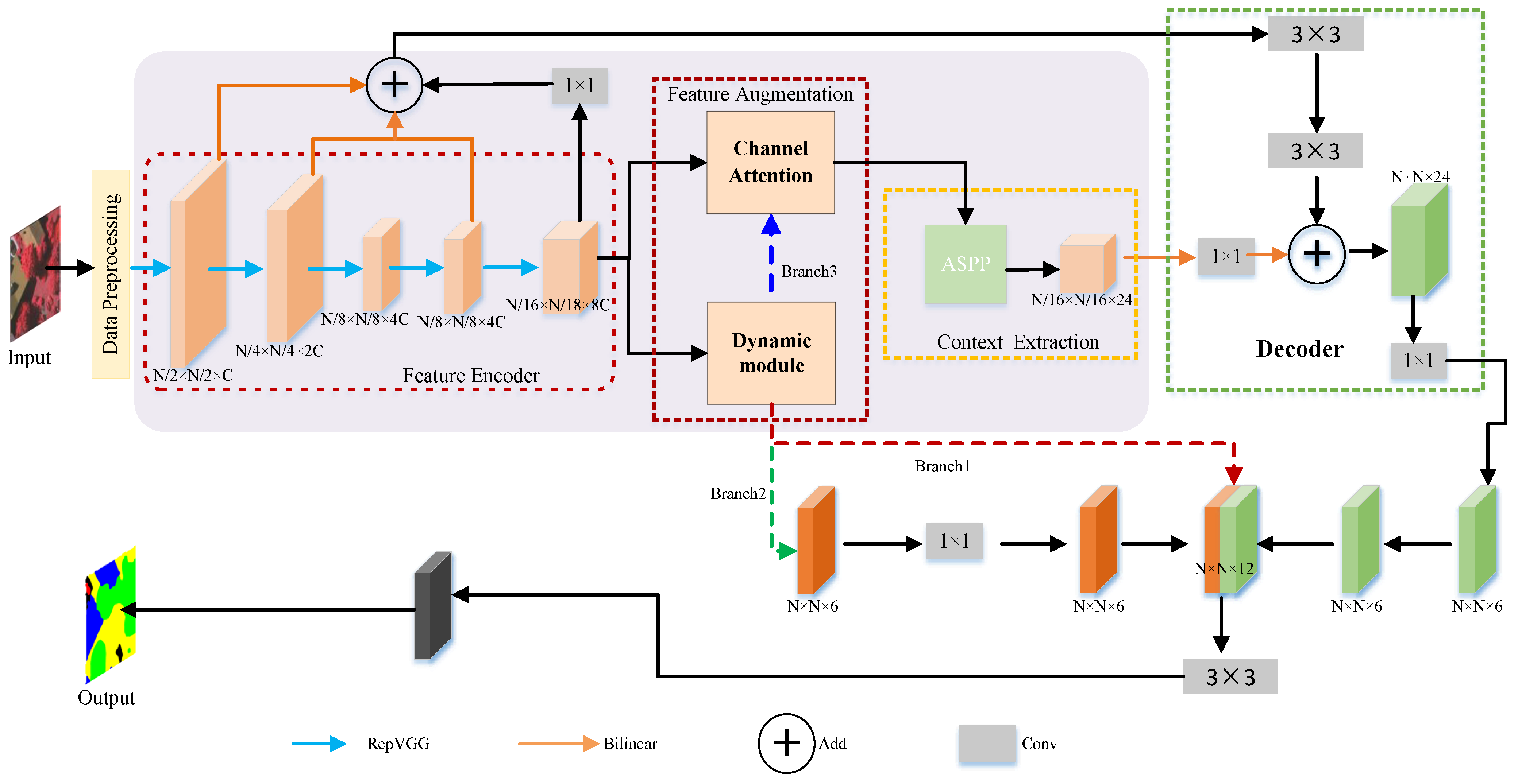
2. Proposed Method
2.1. Encoder Module
2.2. Feature Augmentation
- Calculate the percentage of pixels belonging to small-scale objects in the input feature matrix.
- Compare the calculated percentage with the predefined threshold values.
- Utilize the appropriate feature maps and paths based on the activation of the dynamic module to improve misclassification caused by sparse pixels.
2.3. Context Extractor Module
- The 1 × 1 convolution is a linear transformation of the input feature map.
- The pooling pyramid consists of multiple pooling layers, which are able to reduce the spatial information. In EAD-Net, the dilation rates of the pooling pyramid layers are set to 6, 12, and 18, respectively. These dilation rates allow the pyramid to capture multi-scale spatial information without resolution loss.
- ASPP pooling combines the output of the pooled pyramid and the 1 × 1 convolution. It is able to combine the multi-scale spatial information from the pooling pyramid with transformed features from the 1 × 1 convolution to generate higher-level feature maps. These feature maps contain richer contextual information, which helps the model detect and recognize objects more accurately.
- Input layer: The input layer receives the output of the previous layer or the input feature maps. It applies a 1 × 1 convolution to reduce the number of channels and generate a squeeze feature map.
- Squeeze layer: The squeeze layer is responsible for aggregating the information from each channel of the squeeze feature map. It usually applies a global average pooling operation to compress the spatial information and obtain a 1D feature vector representing the channel-wise statistics.
- Expand layer: The expand layer takes the 1D feature vector from the squeeze layer as input and expands it back into a 2D feature map with the same number of channels as the input feature maps. This is achieved using a 1 × 1 convolution operation.
- Gate layer: The gate layer is designed to learn the correlation between channels and assign different weights to each channel. It uses a sigmoid activation function to generate a binary mask that emphasizes the important channels and suppresses the irrelevant ones. The resulting weighted feature maps are then combined with the expanded feature maps from the expanded layer.
2.4. Decoder Module
- 3 × 3 convolutions: To reduce redundant features, 3 × 3 convolutions are applied to the fused low-level features from the encoder. This step helps to retain essential spatial information while eliminating unnecessary details.
- Fusion with high-level information: The output of the 3 × 3 convolutions is then combined with the high-level context information extracted from the context extraction module. This step enables the fusion of both spatial and semantic information, resulting in a more comprehensive representation of the input image.
- 1 × 1 convolutions: Finally, 1 × 1 convolutions are used to reduce the number of channels, leading to a more compact feature representation.
2.5. Loss Function
3. Implementation
3.1. Dataset Description
3.2. Data Preprocessing
3.3. Implementation Details
3.4. Evaluation Metrics
4. Experimental Comparison and Analysis
4.1. Comparison with the State-of-the-Art
- FCN [21]: FCN (Fully Convolutional Network) was the first method to apply deep convolutional neural networks (DCNNs) for image classification to the semantic segmentation task.
- LR-ASPP [31]: A lightweight network suitable for mobile deployment applications.
- SegNet [24]: A classical semantic segmentation network featuring an encoder-decoder architecture.
- U-Net [22]: Another encoder-decoder structure commonly used for medical image segmentation.
- PSPNet [25]: Pyramid Scene Parsing Network, which is based on the fully convolutional idea of FCN and represents one of the successful improved segmentation models built upon FCN.
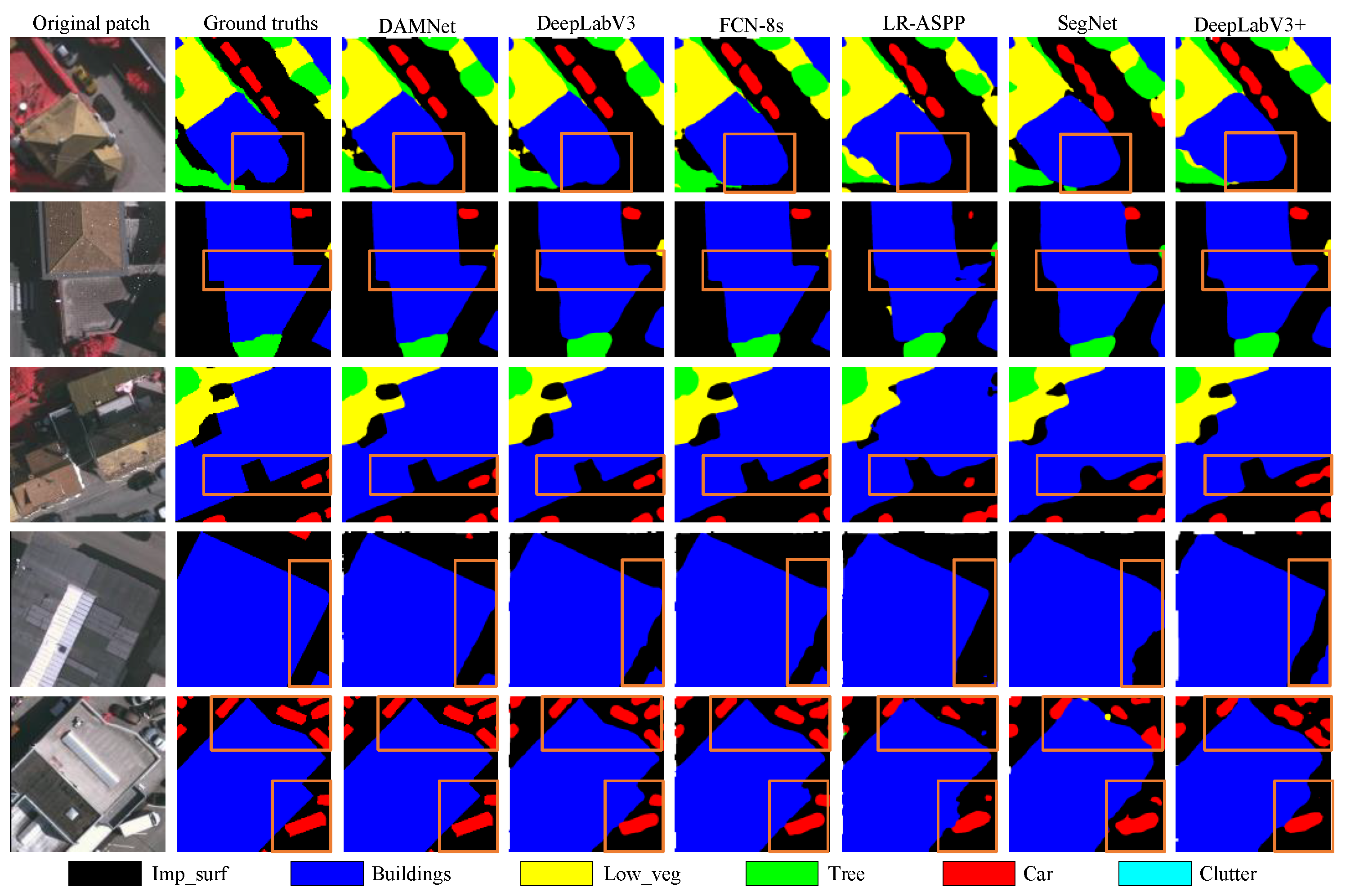
4.2. Experimental Results on the Vaihingen Dataset
4.2.1. Quantitative Evaluation
4.2.2. Qualitative Evaluation
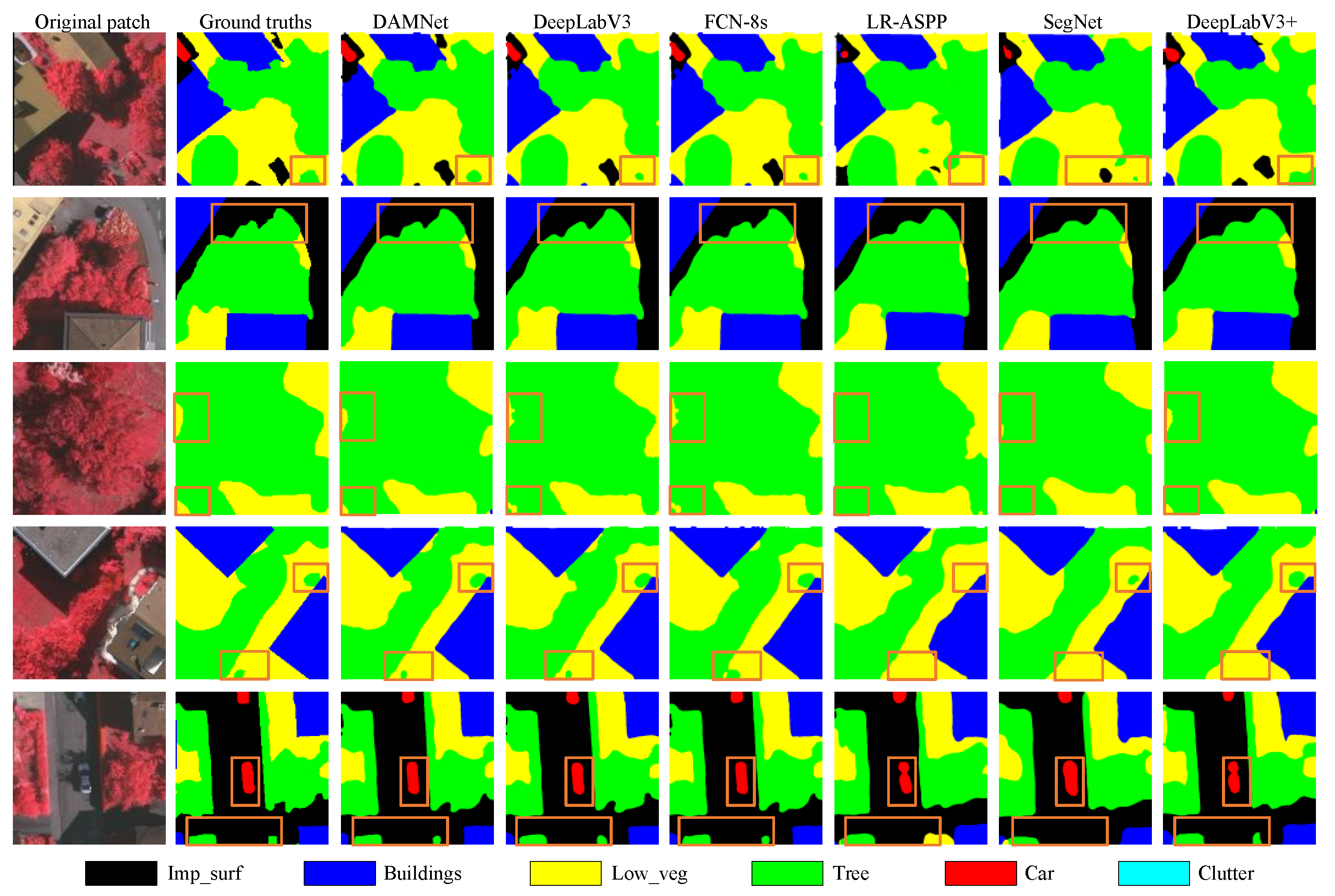
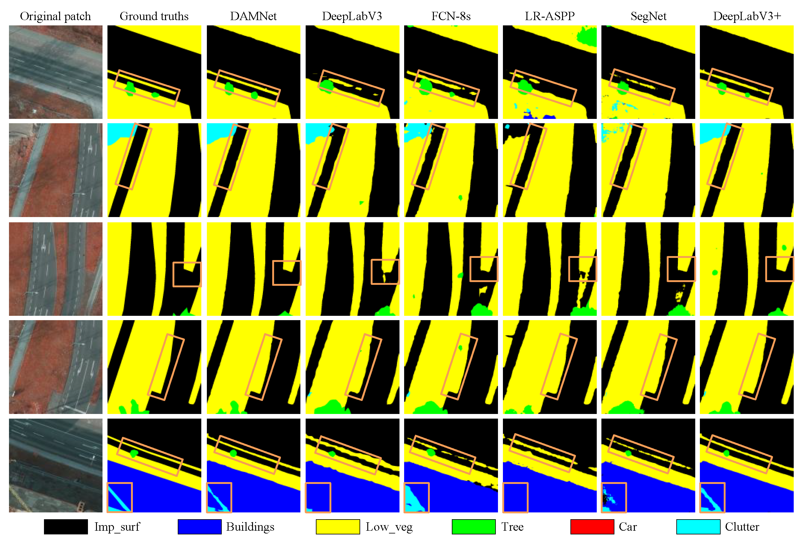
4.3. Experimental Results on the Potsdam Dataset
4.3.1. Quantitative Evaluation
4.3.2. Qualitative Evaluation
4.4. Ablation Study for EAD-Net
4.4.1. Ablation Study for Parameters
4.4.2. Ablation Study of Each Module
4.4.3. Ablation Study of Loss Function
5. Conclusions
Author Contributions
Funding
Data Availability Statement
Conflicts of Interest
References
- He, Q.; Sun, X.; Yan, Z.; Li, B.; Fu, K. Multi-object tracking in satellite videos with graph-based multitask modeling. IEEE Trans. Geosci. Remote Sens. 2022, 60, 1–13. [Google Scholar] [CrossRef]
- Sun, X.; Wang, P.; Yan, Z.; Xu, F.; Wang, R.; Diao, W.; Chen, J.; Li, J.; Feng, Y.; Xu, T.; et al. FAIR1M: A benchmark dataset for fine-grained object recognition in high-resolution remote sensing imagery. ISPRS J. Photogramm. Remote Sens. 2022, 184, 116–130. [Google Scholar] [CrossRef]
- Gu, Y.; Liu, T.; Gao, G.; Ren, G.; Ma, Y.; Chanussot, J.; Jia, X. Multimodal hyperspectral remote sensing: An overview and perspective. Sci. China Inf. Sci. 2021, 64, 1–24. [Google Scholar] [CrossRef]
- Fu, S.; Xu, F.; Jin, Y.Q. Reciprocal translation between SAR and optical remote sensing images with cascaded-residual adversarial networks. Sci. China Inf. Sci. 2021, 64, 1–15. [Google Scholar] [CrossRef]
- Mei, J.; Li, R.J.; Gao, W.; Cheng, M.M. CoANet: Connectivity attention network for road extraction from satellite imagery. IEEE Trans. Image Process. 2021, 30, 8540–8552. [Google Scholar] [CrossRef] [PubMed]
- Rashkovetsky, D.; Mauracher, F.; Langer, M.; Schmitt, M. Wildfire detection from multisensor satellite imagery using deep semantic segmentation. IEEE J. Sel. Top. Appl. Earth Obs. Remote Sens. 2021, 14, 7001–7016. [Google Scholar] [CrossRef]
- Ding, L.; Tang, H.; Liu, Y.; Shi, Y.; Zhu, X.X.; Bruzzone, L. Adversarial shape learning for building extraction in VHR remote sensing images. IEEE Trans. Image Process. 2021, 31, 678–690. [Google Scholar] [CrossRef] [PubMed]
- Kherraki, A.; El Ouazzani, R. Deep convolutional neural networks architecture for an efficient emergency vehicle classification in real-time traffic monitoring. IAES Int. J. Artif. Intell. 2022, 11, 110. [Google Scholar] [CrossRef]
- Li, Y.; Chen, W.; Zhang, Y.; Tao, C.; Xiao, R.; Tan, Y. Accurate cloud detection in high-resolution remote sensing imagery by weakly supervised deep learning. Remote Sens. Environ. 2020, 250, 112045. [Google Scholar] [CrossRef]
- Li, Y.; Zhou, Y.; Zhang, Y.; Zhong, L.; Wang, J.; Chen, J. DKDFN: Domain knowledge-guided deep collaborative fusion network for multimodal unitemporal remote sensing land cover classification. ISPRS J. Photogramm. Remote Sens. 2022, 186, 170–189. [Google Scholar] [CrossRef]
- Peng, D.; Bruzzone, L.; Zhang, Y.; Guan, H.; Ding, H.; Huang, X. SemiCDNet: A semisupervised convolutional neural network for change detection in high resolution remote-sensing images. IEEE Trans. Geosci. Remote Sens. 2020, 59, 5891–5906. [Google Scholar] [CrossRef]
- Zhu, Q.; Guo, X.; Deng, W.; Shi, S.; Guan, Q.; Zhong, Y.; Zhang, L.; Li, D. Land-use/land-cover change detection based on a Siamese global learning framework for high spatial resolution remote sensing imagery. ISPRS J. Photogramm. Remote Sens. 2022, 184, 63–78. [Google Scholar] [CrossRef]
- Zhu, J.; Guo, Y.; Sun, G.; Yang, L.; Deng, M.; Chen, J. Unsupervised domain adaptation semantic segmentation of high-resolution remote sensing imagery with invariant domain-level prototype memory. IEEE Trans. Geosci. Remote Sens. 2023, 61, 1–18. [Google Scholar] [CrossRef]
- Zhou, S.; Feng, Y.; Li, S.; Zheng, D.; Fang, F.; Liu, Y.; Wan, B. DSM-assisted unsupervised domain adaptive network for semantic segmentation of remote sensing imagery. IEEE Trans. Geosci. Remote Sens. 2023, 61, 5608216. [Google Scholar] [CrossRef]
- Yang, Z.; Yan, Z.; Diao, W.; Zhang, Q.; Kang, Y.; Li, J.; Li, X.; Sun, X. Label propagation and contrastive regularization for semi-supervised semantic segmentation of remote sensing images. IEEE Trans. Geosci. Remote Sens. 2023, 61, 5609818. [Google Scholar]
- He, Y.; Wang, J.; Liao, C.; Zhou, X.; Shan, B. MS4D-Net: Multitask-Based Semi-Supervised Semantic Segmentation Framework with Perturbed Dual Mean Teachers for Building Damage Assessment from High-Resolution Remote Sensing Imagery. Remote Sens. 2023, 15, 478. [Google Scholar] [CrossRef]
- Krizhevsky, A.; Sutskever, I.; Hinton, G.E. ImageNet Classification with Deep Convolutional Neural Networks. In Proceedings of the Advances in Neural Information Processing Systems; Pereira, F., Burges, C., Bottou, L., Weinberger, K., Eds.; Curran Associates, Inc.: New York, NY, USA, 2012; Volume 25. [Google Scholar]
- Li, R.; Zheng, S.; Zhang, C.; Duan, C.; Wang, L.; Atkinson, P.M. ABCNet: Attentive bilateral contextual network for efficient semantic segmentation of Fine-Resolution remotely sensed imagery. ISPRS J. Photogramm. Remote Sens. 2021, 181, 84–98. [Google Scholar] [CrossRef]
- Liu, Q.; Kampffmeyer, M.; Jenssen, R.; Salberg, A.B. Dense dilated convolutions’ merging network for land cover classification. IEEE Trans. Geosci. Remote Sens. 2020, 58, 6309–6320. [Google Scholar] [CrossRef]
- Niu, R.; Sun, X.; Tian, Y.; Diao, W.; Feng, Y.; Fu, K. Improving semantic segmentation in aerial imagery via graph reasoning and disentangled learning. IEEE Trans. Geosci. Remote Sens. 2021, 60, 1–18. [Google Scholar] [CrossRef]
- Long, J.; Shelhamer, E.; Darrell, T. Fully convolutional networks for semantic segmentation. In Proceedings of the IEEE Conference on Computer Vision and Pattern Recognition, Boston, MA, USA, 7–12 June 2015; pp. 3431–3440. [Google Scholar]
- Ronneberger, O.; Fischer, P.; Brox, T. U-net: Convolutional networks for biomedical image segmentation. In Proceedings of the Medical Image Computing and Computer-Assisted Intervention–MICCAI 2015: 18th International Conference, Munich, Germany, 5–9 October 2015; pp. 234–241. [Google Scholar]
- Noh, H.; Hong, S.; Han, B. Learning deconvolution network for semantic segmentation. In Proceedings of the IEEE International Conference on Computer Vision, Santiago, Chile, 7–13 December 2015; pp. 1520–1528. [Google Scholar]
- Badrinarayanan, V.; Kendall, A.; Cipolla, R. Segnet: A deep convolutional encoder-decoder architecture for image segmentation. IEEE Trans. Pattern Anal. Mach. Intell. 2017, 39, 2481–2495. [Google Scholar] [CrossRef]
- Zhao, H.; Shi, J.; Qi, X.; Wang, X.; Jia, J. Pyramid scene parsing network. In Proceedings of the IEEE Conference on Computer Vision and Pattern Recognition, Honolulu, HI, USA, 21–26 July 2017; pp. 2881–2890. [Google Scholar]
- Chen, L.C.; Papandreou, G.; Schroff, F.; Adam, H. Rethinking atrous convolution for semantic image segmentation. arXiv 2017, arXiv:1706.05587. [Google Scholar]
- Chen, L.C.; Zhu, Y.; Papandreou, G.; Schroff, F.; Adam, H. Encoder-decoder with atrous separable convolution for semantic image segmentation. In Proceedings of the European Conference on Computer Vision (ECCV), Munich, Germany, 8–14 September 2018; pp. 801–818. [Google Scholar]
- Zhao, H.; Zhang, Y.; Liu, S.; Shi, J.; Loy, C.C.; Lin, D.; Jia, J. Psanet: Point-wise spatial attention network for scene parsing. In Proceedings of the European Conference on Computer Vision (ECCV), Munich, Germany, 8–14 September 2018; pp. 267–283. [Google Scholar]
- Huang, Z.; Wang, X.; Huang, L.; Huang, C.; Wei, Y.; Liu, W. Ccnet: Criss-cross attention for semantic segmentation. In Proceedings of the IEEE/CVF International Conference on Computer Vision, Seoul, Republic of Korea, 27 October–2 November 2019; pp. 603–612. [Google Scholar]
- Fu, J.; Liu, J.; Tian, H.; Li, Y.; Bao, Y.; Fang, Z.; Lu, H. Dual attention network for scene segmentation. In Proceedings of the IEEE/CVF Conference on Computer Vision and Pattern Recognition, Long Beach, CA, USA, 15–20 June 2019; pp. 3146–3154. [Google Scholar]
- Tian, Y.; Chen, F.; Wang, H.; Zhang, S. Real-time semantic segmentation network based on lite reduced atrous spatial pyramid pooling module group. In Proceedings of the 2020 5th International Conference on Control, Robotics and Cybernetics (CRC), IEEE, Wuhan, China, 16–18 October 2020; pp. 139–143. [Google Scholar]
- Wu, T.; Tang, S.; Zhang, R.; Cao, J.; Zhang, Y. Cgnet: A light-weight context guided network for semantic segmentation. IEEE Trans. Image Process. 2020, 30, 1169–1179. [Google Scholar] [CrossRef] [PubMed]
- Yu, C.; Wang, J.; Peng, C.; Gao, C.; Yu, G.; Sang, N. Bisenet: Bilateral segmentation network for real-time semantic segmentation. In Proceedings of the European Conference on Computer Vision (ECCV), Munich, Germany, 8–14 September 2018; pp. 325–341. [Google Scholar]
- Sandler, M.; Howard, A.; Zhu, M.; Zhmoginov, A.; Chen, L.C. Mobilenetv2: Inverted residuals and linear bottlenecks. In Proceedings of the IEEE Conference on Computer Vision and Pattern Recognition, Salt Lake City, UT, USA, 18–23 June 2018; pp. 4510–4520. [Google Scholar]
- Mehta, S.; Rastegari, M.; Caspi, A.; Shapiro, L.; Hajishirzi, H. Espnet: Efficient spatial pyramid of dilated convolutions for semantic segmentation. In Proceedings of the European Conference on Computer Vision (ECCV), Munich, Germany, 8–14 September 2018; pp. 552–568. [Google Scholar]
- Ding, X.; Zhang, X.; Ma, N.; Han, J.; Ding, G.; Sun, J. Repvgg: Making vgg-style convnets great again. In Proceedings of the IEEE/CVF Conference on Computer Vision and Pattern Recognition, Nashville, TN, USA, 20–25 June 2021; pp. 13733–13742. [Google Scholar]
- Chen, L.C.; Collins, M.; Zhu, Y.; Papandreou, G.; Zoph, B.; Schroff, F.; Adam, H.; Shlens, J. Searching for efficient multi-scale architectures for dense image prediction. Adv. Neural Inf. Process. Syst. 2018, 31. [Google Scholar]
- Nekrasov, V.; Chen, H.; Shen, C.; Reid, I. Fast neural architecture search of compact semantic segmentation models via auxiliary cells. In Proceedings of the IEEE/CVF Conference on Computer Vision and Pattern Recognition, Long Beach, CA, USA, 15–20 June 2019; pp. 9126–9135. [Google Scholar]
- Liu, C.; Chen, L.C.; Schroff, F.; Adam, H.; Hua, W.; Yuille, A.L.; Fei-Fei, L. Auto-deeplab: Hierarchical neural architecture search for semantic image segmentation. In Proceedings of the IEEE/CVF Conference on Computer Vision and Pattern Recognition, Long Beach, CA, USA, 15–20 June 2019; pp. 82–92. [Google Scholar]
- Li, Y.; Song, L.; Chen, Y.; Li, Z.; Zhang, X.; Wang, X.; Sun, J. Learning dynamic routing for semantic segmentation. In Proceedings of the IEEE/CVF Conference on Computer Vision and Pattern Recognition, Seattle, WA, USA, 13–19 June 2020; pp. 8553–8562. [Google Scholar]
- Hu, J.; Shen, L.; Sun, G. Squeeze-and-excitation networks. In Proceedings of the IEEE Conference on Computer Vision and Pattern Recognition, Salt Lake City, UT, USA, 18–22 June 2018; pp. 7132–7141. [Google Scholar]
- Bai, H.; Cheng, J.; Su, Y.; Liu, S.; Liu, X. Calibrated Focal Loss for Semantic Labeling of High-Resolution Remote Sensing Images. IEEE J. Sel. Top. Appl. Earth Obs. Remote Sens. 2022, 15, 6531–6547. [Google Scholar] [CrossRef]
- Lin, T.Y.; Goyal, P.; Girshick, R.; He, K.; Dollár, P. Focal loss for dense object detection. In Proceedings of the IEEE International Conference on Computer Vision, Venice, Italy, 22–29 October 2017; pp. 2980–2988. [Google Scholar]
- Doi, K.; Iwasaki, A. The effect of focal loss in semantic segmentation of high resolution aerial image. In Proceedings of the IGARSS 2018–2018 IEEE International Geoscience and Remote Sensing Symposium, IEEE, Valencia, Spain, 22–27 July 2018; pp. 6919–6922. [Google Scholar]


| Ratio (%) | Category | ||||||
|---|---|---|---|---|---|---|---|
| Datasets | Impervious Surface | Building | Low Vegetation | Tree | Car | Clutter | |
| Vaihingen | 28 | 29 | 21 | 23 | 1.2 | 0.8 | |
| Potsdam | 33 | 26 | 22 | 14 | 1.3 | 3.7 | |
| Methods | ||||||||
|---|---|---|---|---|---|---|---|---|
| FCN-8s [21] | DeepLabV3 [26] | LR-ASPP [31] | SegNet [24] | U-Net [22] | PSP-Net [25] | DeepLabV3+ [27] | EAD-Net | |
| Backbone | ResNet50 | ResNet50 | MobileNetV3 | ResNet50 | MobileNetV3 | ResNet50 | MobileNetV3 | ResNet50 |
| mPA | 91.93 | 92.01 | 78.90 | 82.14 | 64.84 | 67.96 | 85.87 | 92.27 |
| mIoU | 86.08 | 86.11 | 69.98 | 74.86 | 61.54 | 70.15 | 76.61 | 87.38 |
| Method | PA(%) | ||||||||
|---|---|---|---|---|---|---|---|---|---|
| Category | FCN-8s [21] | DeepLabV3 [26] | LR-ASPP [31] | SegNet [24] | U-Net [22] | PSP-Net [25] | DeepLabV3+ [27] | EAD-Net | |
| Imp_ surf | 94.26 | 94.03 | 87.88 | 91.73 | 75.11 | 70.28 | 90.79 | 94.28 | |
| Building | 94.83 | 95.11 | 91.17 | 85.92 | 76.14 | 77.63 | 95.34 | 95.66 | |
| Low_ veg | 89.77 | 89.68 | 81.22 | 82.22 | 66.14 | 73.22 | 84.38 | 89.87 | |
| Tree | 90.76 | 91.27 | 82.86 | 87.83 | 68.07 | 63.29 | 84.93 | 91.43 | |
| Car | 85.79 | 85.04 | 61.66 | 54.55 | 50.32 | 59.47 | 69.47 | 88.91 | |
| Clutter | 96.18 | 96.94 | 68. 61 | 90.59 | 53.23 | 63.88 | 90.29 | 96.17 | |
| mPA (%) | 91.93 | 92.01 | 78.90 | 82.14 | 64.84 | 67.96 | 85.87 | 92.72 | |
| Method | IoU(%) | ||||||||
|---|---|---|---|---|---|---|---|---|---|
| Category | FCN-8s [21] | DeepLabV3 [26] | LR-ASPP [31] | SegNet [24] | U-Net [22] | PSP-Net [25] | DeepLabV3+ [27] | EAD-Net | |
| Imp_ surf | 88.35 | 88.84 | 78.39 | 86.44 | 69.24 | 70.16 | 84.77 | 86.70 | |
| Building | 91.33 | 91.55 | 83.64 | 85.07 | 64.56 | 78.68 | 90.63 | 91.64 | |
| Low_ veg | 82.31 | 82.52 | 69.10 | 72.72 | 61.37 | 69.74 | 72.90 | 83.45 | |
| Tree | 81.66 | 82.37 | 67.82 | 72.93 | 57.26 | 68.52 | 70.66 | 83.12 | |
| Car | 78.04 | 77.36 | 53.07 | 50.55 | 46.11 | 60.39 | 59.52 | 84.65 | |
| Clutter | 94.79 | 94.04 | 67.88 | 81.42 | 70.70 | 73.41 | 81.17 | 94.69 | |
| mIoU (%) | 86.08 | 86.11 | 69.98 | 74.86 | 61.54 | 70.15 | 76.61 | 87.38 | |
| Methods | ||||||||
|---|---|---|---|---|---|---|---|---|
| FCN-8s [21] | DeepLabV3 [26] | LR-ASPP [31] | SegNet [24] | U-Net [22] | PSP-Net [25] | DeepLabV3+ [27] | EAD-Net | |
| Backbone | ResNet50 | ResNet50 | MobileNetV3 | ResNet50 | MobileNetV3 | ResNet50 | MobileNetV3 | ResNet50 |
| mPA | 89.29 | 88.29 | 84.75 | 87.85 | 66.82 | 90.37 | 94.69 | 96.27 |
| mIoU | 81.80 | 79.92 | 75.52 | 80.65 | 60.35 | 65.58 | 89.93 | 93.10 |
| Method | PA(%) | ||||||||
|---|---|---|---|---|---|---|---|---|---|
| Category | FCN-8s [21] | DeepLabV3 [26] | LR-ASPP [31] | SegNet [24] | U-Net [22] | PSP-Net [25] | DeepLabV3+ [27] | EAD-Net | |
| Imp_ surface | 93.32 | 92.49 | 90.67 | 93.49 | 76.60 | 94.51 | 96.89 | 97.82 | |
| Building | 97.28 | 97.10 | 96.21 | 97.64 | 77.23 | 97.99 | 98.67 | 99.15 | |
| Low_ veg | 89.54 | 88.81 | 87.91 | 89.61 | 65.14 | 90.90 | 94.96 | 96.63 | |
| Tree | 85.38 | 83.56 | 76.31 | 83.19 | 62.39 | 87.60 | 92.52 | 94.86 | |
| Car | 90.24 | 87.71 | 85.09 | 88.72 | 58.77 | 87.26 | 92.03 | 93.67 | |
| Clutter | 79.98 | 80.05 | 72.31 | 74.42 | 60.78 | 83.95 | 92.92 | 95.50 | |
| mPA (%) | 89.29 | 88.29 | 84.75 | 87.85 | 66.82 | 90.37 | 94.69 | 96.27 | |
| Method | IoU(%) | ||||||||
|---|---|---|---|---|---|---|---|---|---|
| Category | FCN-8s [21] | DeepLabV3 [26] | LR-ASPP [31] | SegNet [24] | U-Net [22] | PSP-Net [25] | DeepLabV3+ [27] | EAD-Net | |
| Imp_ surf | 87.50 | 86.73 | 83.44 | 87.17 | 63.49 | 89.25 | 93.61 | 95.51 | |
| Building | 94.49 | 94.15 | 91.87 | 94.58 | 70.22 | 95.59 | 97.55 | 98.28 | |
| Low_ veg | 79.34 | 77.70 | 73.27 | 78.43 | 74.04 | 82.40 | 89.93 | 93.21 | |
| Tree | 75.56 | 72.96 | 66.25 | 73.76 | 65.38 | 79.04 | 86.40 | 90.88 | |
| Car | 82.95 | 78.47 | 75.10 | 82.14 | 58.63 | 79.19 | 86.93 | 88.96 | |
| Clutter | 70.96 | 69.80 | 63.02 | 67.05 | 55.19 | 75.91 | 87.49 | 91.73 | |
| mIoU (%) | 81.80 | 79.97 | 75.49 | 80.52 | 64.49 | 83.56 | 90.35 | 93.10 | |
| Backbone | |||||
|---|---|---|---|---|---|
| ResNet 18 | ResNet 34 | ResNet 50 | ResNet 101 | ||
| FLOPs (G) | 31.854047232 | 41.543938048 | 46.984892416 | 66.486308864 | |
| Vaihingen | Params (M) | 16.803289 | 26.911449 | 40.940505 | 59.932633 |
| mIoU (%) | 84.21 | 85.66 | 87.38 | 88.93 | |
| FLOPs (G) | 36.45278166 | 43.18914782 | 48.33298745 | 70.83546797 | |
| Potsdam | Params (M) | 18.065447 | 19.136658 | 42.588741 | 64.2938174 |
| mIoU (%) | 88.29 | 90.06 | 93.10 | 94.37 | |
| ASPP | SE Module | Dynamic Module | Category | |||||||||||
|---|---|---|---|---|---|---|---|---|---|---|---|---|---|---|
| Imp_ surf | Building | Low_ veg | Tree | Car | Clutter | |||||||||
| PA | IoU | PA | IoU | PA | IoU | PA | IoU | PA | IoU | PA | IoU | |||
| ✓ | 90.58 | 83.12 | 91.04 | 88.22 | 85.34 | 78.26 | 85.44 | 78.64 | 80.22 | 81.58 | 92.78 | 90.71 | ||
| ✓ | ✓ | 93.27 | 85.66 | 93.51 | 90.17 | 88.06 | 81.48 | 89.14 | 81.18 | 85.96 | 83.44 | 94.49 | 93.06 | |
| ✓ | ✓ | 93.22 | 85.16 | 93.24 | 90.88 | 88.24 | 81.39 | 88.67 | 81.09 | 86.33 | 83.16 | 95.23 | 92.88 | |
| ✓ | ✓ | ✓ | 94.28 | 86.70 | 95.66 | 91.64 | 89.87 | 83.45 | 91.43 | 83.12 | 88.91 | 84.65 | 96.17 | 94.69 |
| ASPP | SE Module | Dynamic Module | Category | |||||||||||
|---|---|---|---|---|---|---|---|---|---|---|---|---|---|---|
| Imp_ surf | Building | Low_ veg | Tree | Car | Clutter | |||||||||
| PA | IoU | PA | IoU | PA | IoU | PA | IoU | PA | IoU | PA | IoU | |||
| ✓ | 92.33 | 95.08 | 93.74 | 88.22 | 89.54 | 92.68 | 86.33 | 90.41 | 84.72 | 88.33 | 87.42 | 90.71 | ||
| ✓ | ✓ | 94.51 | 95.63 | 96.55 | 90.17 | 91.20 | 94.39 | 88.47 | 92.88 | 86.29 | 90.15 | 89.54 | 92.05 | |
| ✓ | ✓ | 94.26 | 96.61 | 96.93 | 90.88 | 90.77 | 94.78 | 89.15 | 93. 60 | 87.11 | 90.56 | 90.26 | 93.66 | |
| ✓ | ✓ | ✓ | 97.82 | 95.51 | 99.15 | 98.28 | 96.63 | 93.21 | 94.86 | 90.88 | 93.67 | 88.96 | 95.50 | 91.73 |
Disclaimer/Publisher’s Note: The statements, opinions and data contained in all publications are solely those of the individual author(s) and contributor(s) and not of MDPI and/or the editor(s). MDPI and/or the editor(s) disclaim responsibility for any injury to people or property resulting from any ideas, methods, instructions or products referred to in the content. |
© 2024 by the authors. Licensee MDPI, Basel, Switzerland. This article is an open access article distributed under the terms and conditions of the Creative Commons Attribution (CC BY) license (https://creativecommons.org/licenses/by/4.0/).
Share and Cite
Hu, Q.; Wang, F.; Li, Y. EAD-Net: Efficiently Asymmetric Network for Semantic Labeling of High-Resolution Remote Sensing Images with Dynamic Routing Mechanism. Remote Sens. 2024, 16, 1478. https://0-doi-org.brum.beds.ac.uk/10.3390/rs16091478
Hu Q, Wang F, Li Y. EAD-Net: Efficiently Asymmetric Network for Semantic Labeling of High-Resolution Remote Sensing Images with Dynamic Routing Mechanism. Remote Sensing. 2024; 16(9):1478. https://0-doi-org.brum.beds.ac.uk/10.3390/rs16091478
Chicago/Turabian StyleHu, Qiongqiong, Feiting Wang, and Ying Li. 2024. "EAD-Net: Efficiently Asymmetric Network for Semantic Labeling of High-Resolution Remote Sensing Images with Dynamic Routing Mechanism" Remote Sensing 16, no. 9: 1478. https://0-doi-org.brum.beds.ac.uk/10.3390/rs16091478